Bose-Einstein condensation of rubidium atoms in a triaxial TOP-trap

Abstract

We report the results of experiments with Bose-Einstein condensates of rubidium atoms in a triaxial TOP-trap, presenting measurements of the condensate fraction and the free expansion of a condensate released from the trap. The experimental apparatus and the methods used to calibrate the magnetic trapping fields are discussed in detail. Furthermore, we compare the performance of our apparatus with other TOP-traps and discuss possible limiting factors for the sizes of condensates achievable in such traps.

1 Introduction

Since the first observations of Bose-Einstein condensation (BEC) in dilute alkali gases [1, 2, 3], experimental as well as theoretical studies of degenerate quantum gases have been published at an astonishing rate [4, 5]. Far beyond the mere realization and detection of BEC, experimenters have investigated the static and dynamic properties of Bose-Einstein condensates and have gained considerable control over these macroscopic quantum objects, up to the point of creating coherent beams of matter waves - atom lasers, in other words. In spite of these early successes, experimental BEC is still a growing and thriving field, and much research needs to be done in order to test the vast number of theoretical predictions made in the last few years.

In this paper, we present the experimental apparatus used to create BECs of rubidium atoms in a triaxial time-orbiting-potential (TOP) trap [6]. To the best of our knowledge, while the triaxial TOP trap has been used in BEC experiments on sodium [7], no previous application to rubidium has been reported. We describe in some detail the experimental parameters of our system and compare the performance of our apparatus with those of other groups using similar setups. Section 2 presents the experimental set-up, with emphasis on the original parts for the rubidium cooling and transfer between the two magneto-optical traps. Section 3 reports the parameters for the loading and evaporative cooling phases required to produce the condensate. Moreover, the gain in phase-space density achieved during the evaporation phases has been measured. In the following sections the results of various measurements on the condensate are reported. The final phase-space density, number of atoms and temperatures associated to the different condensates are presented. Furthermore, the expansion of the condensate following a switch-off of the magnetic trap has been studied and compared to different theoretical models. Finally, we describe different methods used for precise measurements of the magnetic fields. In this way, we obtained an accurate calibration which was needed as an input parameter for a theoretical model simulating the motion of the atomic cloud [8].

2 Experimental setup

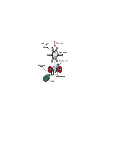
Figure 1: Setup of our experiment. The atoms are transferred from the upper to the lower MOT by a push beam which is briefly flashed on after loading the upper MOT for $160\,\mathrm{ms}$. This cycle is repeated about $200$ times. For clarity, the laser beams for the lower MOT are not shown here.

Our experimental apparatus is based on a double-MOT system with a TOP-trap. The design of the vacuum system and the positioning of the coils are shown in figure 1. Owing to the arrangement of the quadrupole coils and the TOP-coils, our trap is triaxial without cylindrical symmetry. In the following, we give a brief overview of the specifications of our system.
Vacuum system: Our vacuum system is composed of two quartz cells connected by a glass tube of inner diameter $12\,\mathrm{mm}$ and length $20\,\mathrm{cm}$ (see figure 1). At the upper end of the glass tube, a graphite tube of length $6\,\mathrm{cm}$ and inner diameter $5\,\mathrm{mm}$ is inserted in order to enhance differential pumping. The upper cell is connected to a $20\,\mathrm{ls^{-1}}$ ion pump, whereas the lower cell is pumped on by a $40\,\mathrm{ls^{-1}}$ ion pump in conjunction with a Ti-sublimation pump. In this way, a pressure gradient is created between the two cells with the pressure in the upper cell being of the order of $10^{-8}\,\mathrm{Torr}$ and that of the lower cell below $10^{-10}\,\mathrm{Torr}$. The upper cell also contains two Rb dispensers (SAES getters) which we operate at $3.0\,\mathrm{A}$.
Lasers: The laser light for the upper and lower MOTs is derived from a MOPA (tapered amplifier) injected in turn by a $50\,\mathrm{mW}$ diode laser. Under typical conditions we extract up to $320\,\mathrm{mW}$ of useful output from this system, which is then frequency-shifted by acousto-optic modulators (AOMs) and mode-cleaned by optical fibres. In this way, we create up to $60\,\mathrm{mW}$ of laser power for the upper MOT and $15\,\mathrm{mW}$ for the lower MOT. The repumping light for both the upper and the lower MOT is derived from a $75\,\mathrm{mW}$ diode laser, yielding about $9\,\mathrm{mW}$ of total power after passage through all the optical elements. The injecting laser for the MOPA and the repumping laser are both injected by $50\,\mathrm{mW}$ grating stabilized diode lasers locked to Rb absorption lines.
Magnetic trap: Our TOP-trap consists of a pair of quadrupole coils capable of producing field gradients $2b^{\prime}$ (along the symmetry axis) in excess of $1000\,\mathrm{Gcm^{-1}}$ for maximum currents of about $230\,\mathrm{A}$, and two pairs of TOP-coils. The quadrupole coils are water-cooled and are oriented horizontally (along the $x$-axis, see fig. 1) about the lower glass cell of our apparatus. A combination of IGBTs and varistors is used for fast switching of the current provided by a programmable current source (HP6882) whilst protecting the circuits from damage due to high voltages induced during switch-off. In this way we are able to switch off the quadrupole field within less than $50\,\mathrm{\mu s}$ even for the largest field gradients. The rotating bias field $B_{0}$ is created by two pairs of coils: One (circular) pair is incorporated into the quadrupole coils, whilst the other (rectangular) pair is mounted along the $y$-axis. Within the adiabatic and harmonic approximations, for an atom with mass $m$ and magnetic moment $\mu$ this results in a triaxial time-orbiting potential $V_{TOP}$ given by

$$V_{TOP}=\frac{4\pi^{2}m}{2}\left(\nu_{x}^{2}x^{2}+\nu_{y}^{2}y^{2}+\nu_{z}^{2}z^{2}\right)$$ (1)

with the following frequencies along the three axes of the trap in the ratio $2:1:\sqrt{2}$, as introduced in [7]:

$$\nu_{x} = \frac{1}{2\pi}\sqrt{\frac{2\mu}{mB_{0}}}b^{\prime}$$ (2)

$$\nu_{y} = \frac{1}{2\pi}\sqrt{\frac{\mu}{2mB_{0}}}b^{\prime}$$ (3)

$$\nu_{z} = \frac{1}{2\pi}\ \sqrt{\frac{\mu}{mB_{0}}}b^{\prime}.$$ (4)

The anharmonic and gravitational effects neglected in this approximation will be discussed in section 5. The TOP-coils in our experiment can produce a bias field $B_{0}$ of up to $30\,\mathrm{G}$ and are operated at a frequency of $10\,\mathrm{kHz}$.
Imaging: Detection of the condensates is done by shadow imaging using a near-resonant probe beam. The absorptive shadow cast by the atoms is imaged onto a CCD-camera. With a camera pixel size of $9\,\mathrm{\mu m}$ and a magnification of about $1.2$, we achieve a resolution of just over $7\,\mathrm{\mu m}$. Most of our measurements are made after a few milliseconds of free fall of the released condensate, when typical dimensions are of the order of $10-30\,\mathrm{\mu m}$.

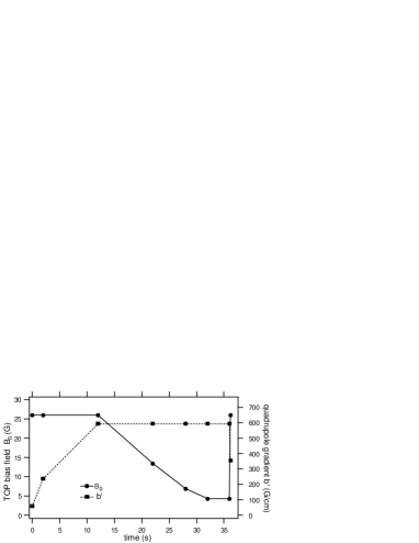
Figure 2: Compression and evaporative cooling in our TOP. Shown here are the ramps for the bias field $B_{0}$ and the gradient along the $z$-axis, $b^{\prime}$. The condensate is formed at t= 37 s, where both $B_{0}$ and $b^{\prime}$ are ramped for condensate imaging.

3 Evaporative cooling and creation of the condensate

A typical experimental cycle from the initial collection of atoms in the upper MOT to the creation of a BEC is as follows. First, we load about $5\times 10^{7}$ $\mathrm{Rb}$ atoms into the lower MOT by repeatedly (up to 200 times) loading the upper MOT for $\approx 160\,\mathrm{ms}$ and then flashing on a near-resonant push beam that accelerates the atoms down the connecting tube. Once the lower MOT has been filled, a $30\,\mathrm{ms}$ compressed-MOT phase increases the density of the cloud, which is then cooled further to about $15\,\mathrm{\mu K}$ by a molasses phase of a few milliseconds. At this point, the molasses beams are switched off and an optical pumping beam is flashed on five times for $20\,\mathrm{\mu s}$, synchronized with the rotating bias field of $1\,\mathrm{G}$ to define a quantization axis, in order to transfer the atoms into the $|F=2,m_{F}=2\rangle$ Zeeman substate desired for magnetic trapping. Transfer into the TOP-trap is then effected by simultaneously switching on the rotating bias field (at its maximum value of about $25\,\mathrm{G}$) and the quadrupole field (at a value for the gradient chosen such as to achieve mode-matching between the initial cloud of atoms and the resulting magnetic trap frequencies). The subsequent evaporative cooling ramps for the quadrupole and the bias fields are shown schematically in figure 2. After an adiabatic compression phase, during which the quadrupole gradient is increased to its maximum value, the bias field amplitude is ramped down linearly. In this way, we perform circle-of-death evaporative cooling down to a bias field of around $4\,\mathrm{G}$. Next, at a constant bias field, we switch on a radio-frequency field, scanning its frequency exponentially from $6.5\,\mathrm{MHz}$ down to around $3.2\,\mathrm{MHz}$, which we find to be the threshold for condensation for our system. At threshold, we have up to $3\times 10^{4}$ atoms in the condensate/thermal cloud-conglomerate. Continuing rf-evaporation still further yields pure condensates of up to $1-2\times 10^{4}$ atoms with no discernible thermal fraction. The value for the bias field at which we switch from circle-of-death to rf-evaporation was chosen by maximizing the final condensate number. The approach to BEC is illustrated graphically in figure 3, in which the phase-space density is plotted as a function of the number of atoms.
Before imaging the condensate, we adiabatically change the trap frequency by ramping the bias field and the quadrupole gradient in $200\,\mathrm{ms}$. In this way, we can choose the frequency of the trap in which we wish to study the condensate. Thereafter, both fields are switched off on a timescale of $20-50\,\mathrm{\mu s}$ for the quadrupole field and $100-200\,\mathrm{\mu s}$ for the bias field. Owing to these short timescales, the change in trap frequency during the switching can essentially be neglected as typical oscillation periods in the trap are larger than $10\,\mathrm{ms}$. In fact, we were able to observe non-adiabatic motion of the trapped condensates at the frequency of the rotating bias field [8].

Figure 3: Phase-space density in the triaxial TOP-trap as a function of atom number. The slope of the linear fit in the log-log plot corresponds to a gain in phase-space density of a factor 100 for a reduction in the atom number by a factor 10.

4 Experimental results

In the following, we briefly summarize some initial measurements made on the condensates obtained with our apparatus.

4.1 Evidence for condensation and condensate fraction

In order to find the threshold for condensation, the RF-frequency in the final evaporation step is lowered whilst monitoring the properties of the atom cloud (through shadow imaging after $3\,\mathrm{ms}$ of free expansion). At the threshold, the tell-tale signs of condensation, namely a sudden increase in peak density and the onset of a bimodal distribution, begin to appear. Figure 4 shows plots of the peak density normalized with respect to the number of atoms (which removes the considerable experimental jitter especially in the condensed regime) and the condensate fraction as a function of the final RF-frequency. The condensate fraction is determined from a bimodal fit to single pixel rows of the absorption picture, and it is evident in the two plots that condensation sets in at a final frequency of about $3.2\,\mathrm{MHz}$, corresponding to a temperature of $365\,\mathrm{nK}$ as calculated from the ballistic expansion of the cloud, and a peak density of $\approx 5\times 10^{11}\,\mathrm{cm^{-3}}$. From this, we calculate a phase-space density of $2.5$ at the threshold, in agreement with theoretical predictions. Using the expression $k_{B}T_{0}=\hbar\bar{\omega}(N/\zeta(3))^{1/3}$ (valid in the non-interacting approximation and with $\bar{\omega}$ equal to the geometric mean of the three trap frequencies) with $N=10^{4}$ atoms at the threshold [9], we find $T_{0}\approx 400\,\mathrm{nK}$ in good agreement with our observed threshold temperature.
We note here that, unlike in the case of a static trap, for a TOP-trap there is no strict proportionality between $\nu_{cut}-\nu_{0}$ and $k_{B}T_{cut}$, where $\nu_{cut}$ is the frequency of the RF-field, $\nu_{0}$ is the resonance frequency at the bottom of the trap, and $T_{cut}$ is the equivalent cut temperature. A simple calculation considering the maximum instantaneous field at the resonance shell shows that, for low temperatures,

$$\nu_{cut}-\nu_{0}=\frac{g_{F}}{h}\bigl{(}2k_{B}T_{cut}\mu B_{0}\bigr{)}^{1/2}.$$ (5)

This geometric average between the thermal cut energy $k_{B}T_{cut}$ and the magnetic energy in the bias field $\mu B_{0}$ of the TOP-trap leads to a considerably more accurate control of the cut energy in a TOP-trap. For instance, at a bias field of $B_{0}=4\,\mathrm{G}$, a frequency difference $\nu_{cut}-\nu_{0}$ of $350\,\mathrm{kHz}$ corresponds to a cut energy $T_{cut}$ of only $1.2\,\mathrm{\mu K}$, whereas the same frequency difference in a static trap leads to $T_{cut}=34\,\mathrm{\mu K}$.

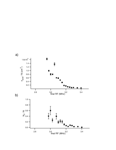
Figure 4: Normalized peak density of the trapped atomic cloud (a) and condensate fraction (b) as a function of the final RF-frequency. From the two graphs it is evident that condensation occurs at a final RF-frequency of about $3.2\,\mathrm{MHz}$. The bottom of the trap is located at a final frequency of $2.75\,\mathrm{MHz}$. Only data obtained from absorption pictures in which a non-condensed fraction was clearly discernible were included in plot (b).

4.2 Free expansion of the condensate

One way of obtaining information on the properties of a Bose-Einstein condensate is to investigate its behaviour after it is released from the trap. Its subsequent evolution is then monitored by taking absorption images after a variable time-of-flight. The results of such measurements on a condensate released from a trap with $\nu_{z}=363\,\mathrm{Hz}$ are shown in figure 5. Theoretically, the expansion of a condensate has been investigated by several authors, and analytical expressions for the condensate width and its aspect ratio as a function of time can be found in special cases. Figure 5 shows the predictions of a model based on the Thomas-Fermi approximation [10], in which the energy of the condensate is dominated by the mean-field interaction between the atoms, as well as the theoretical expansion of a ground-state harmonic oscillator wavefunction, for which interactions are neglected entirely. Clearly, our experimental data agree with neither of these two extremes. This is to be expected, as the sizes of our condensates, with typically a few thousand atoms in a pure condensate, are rather small and therefore do not fully satisfy the conditions for a Thomas-Fermi treatment. It is, therefore, necessary to compare our data with a numerical integration of the full Gross-Pitaevskii equation. The results of such an integration are also plotted in figure 5. As expected, they lie between the two extreme models and fit our data reasonably well. It is clear, however, that our condensate number is so low that the interaction term in the Gross-Pitaevskii equation is almost negligible and the numerical results are close to the pure harmonic oscillator case.

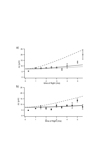
Figure 5: Free expansion of a Bose-Einstein condensate released from a triaxial TOP-trap. The number of atoms in the (pure) condensates was around $10^{3}$. Also shown are the theoretical predictions for a harmonic oscillator wave-packet (dotted line), the Thomas-Fermi limit (dashed line), and a numerical integration of the full Gross-Pitaevskii equation (solid line). The theoretical graphs are corrected for a finite resolution of $7\,\mathrm{\mu m}$.

5 Calibration of the magnetic fields

In many applications of magnetic traps, it is sufficient to describe the trap by its characteristic frequencies for dipolar oscillations of atomic clouds. In such a measurement, one applies a magnetic field along a chosen axis for a short time, thus giving a kick to the (initially stationary) atomic cloud, and monitors the subsequent oscillations of the atoms. With a judicious choice of the points in time at which the position of the cloud is sampled, one can achieve frequency measurements with uncertainties well below the percent level. Deducing absolute values of the magnetic field gradient and the bias field from these measurements with similar accuracy, however, is not so straightforward. The main incentive for us to accurately measure these absolute values was that we needed them as input parameters for numerical simulations of non-adiabatic motion in the TOP-trap [8]. In the following, we shall briefly describe several methods we used to measure absolute values for both the quadrupole gradient and the bias field and indicate the uncertainties associated with these measurements. For the most part, the measurements were carried out with condensates, which facilitated the determination of the position of the atomic cloud.
In the first method, we measure the vibrational frequencies $\tilde{\nu_{x}}$ and $\tilde{\nu_{z}}$ along the $x$- and $z$-axes, respectively, exciting the dipolar modes along these two directions simultaneously. In order to be able to use theoretical formulas derived in the harmonic approximation taking into account the effect of gravity, we have calculated the anharmonic corrections up to fourth order, including cross-terms, following the scheme presented by Ensher [11]. The results reported in Appendix A allow us to deduce from our measured frequencies the corresponding values in the harmonic limit (equivalent to infinitesimal oscillation amplitudes; typical amplitudes in our experiment are between $20\,\mathrm{\mu m}$ and $60\,\mathrm{\mu m}$.). Those anharmonic corrections can be up to $1\%$ of the measured values and are, therefore, essential if an accuracy in the magnetic field below the percent level is desired. The quadrupole gradient can be calculated directly from the ratio $\tilde{\nu_{x}}/{\tilde{\nu}_{z}}$ given by in the harmonic approximation with the gravitational corrections by

$$\frac{\tilde{\nu_{x}}}{\tilde{\nu_{z}}}=\sqrt{2}\sqrt{\frac{1+\eta^{2}}{1-\eta^{2}}}$$ (6)

Here, $\eta$, defined by

$$\eta=\frac{\mu b^{\prime}}{mg}$$ (7)

measures the ratio of magnetic and gravitational forces along the $z$-axis. It is interesting to note that in the triaxial TOP the gravity corrections are equal to those derived for a cylindrically symmetric TOP-trap [11]. Re-substitution of the value for $b^{\prime}$ thus retrieved along with either of the two frequencies into the expression for $\tilde{\nu_{x}}$ or $\tilde{\nu_{z}}$ then yields a value for $B_{0}$. For instance, $\tilde{\nu_{z}}$ is given by

$$\tilde{\nu_{z}}=\frac{1}{2\pi}\sqrt{\frac{\mu}{mB_{0}}}b^{\prime}\left(1-\eta^{2}\right)^{3/4}.$$ (8)

In order to check the obtained values for $B_{0}$ and $b^{\prime}$ by independent methods not relying on the calculated frequencies for a TOP-trap, we use two separate strategies. In one method, the quadrupole gradient is measured by first trapping and evaporatively cooling atoms in the presence of both the quadrupole and the bias fields. Then, the bias field is switched off, which shifts the centre of the quadrupole potential with respect to the TOP-potential. The quadrupole gradient is subsequently determined by measuring the acceleration of the atoms and subtracting the acceleration due to gravity. In this way, $b^{\prime}$ can be determined with a relative error of less than $1\%$. An independent measurement of the bias field $B_{0}$ is made by switching off the quadrupole field after the atoms have been cooled in the TOP whilst leaving the bias field on. A short ($100-500\,\mathrm{\mu s}$) RF-pulse is then applied to the atoms at a given frequency, and the number of atoms remaining in the original trapped state is measured after turning the quadrupole field back on (about $1\,\mathrm{ms}$ after switching it off). When the frequency of the RF-pulse matches the Zeeman-splitting due to the bias field, atoms are transferred into untrapped Zeeman-substates and hence lost from the trap. Using this method, we found two different values of the RF-pulses for which atoms were lost from the trap, indicating that there is a slight asymmetry between the magnetic fields produced by the two pairs of TOP-coils. Measuring $B_{0}$ with this method proved to be less reliable than with the method described above, but yielded the same value for the bias field to within $5\%$.

6 Condensate numbers in TOP-traps

In our experimental apparatus, we obtain condensates containing up to a few $10^{4}$ atoms, starting from typical MOT numbers of about $5\times 10^{7}$. Extrapolating this linearly, one would expect to achieve condensate numbers of up to $10^{6}$ for an initial number of $5\times 10^{9}$ atoms in the MOT. In the literature, however, one typically finds reports of some $10^{5}$ atoms in the condensate under such circumstances. In figure 6 we have plotted typical figures for the MOT and the condensate numbers for a few groups using rubidium TOP-traps. Evidently, the reported condensate numbers do not scale linearly with the MOT numbers. Instead, they can be fitted roughly by a square-root law. Varying the MOT numbers in our own experiment, we find a similar behaviour on a smaller scale. We discovered this when trying to increase the size of our condensates and found that the main limiting factor comes from the compression phase after loading the magnetic trap. Above a certain number of atoms loaded into the MOT, we saw next to no increase in the atom number after compression (or, for that matter, in the condensate) when increasing the initial number of atoms. As in [12], we attribute this to an unfavourable ratio of the size of the initial cloud and the circle-of-death radius. When the cloud becomes too big, the circle-of-death cuts into it during compression and thus any increase in the atom number is eaten up by this cutting. This may be a limiting mechanism for most groups and could explain the law of diminishing returns that is evident in figure 6. In this context it is interesting to note that, for instance, the JILA group uses a much higher bias field ($50\,\mathrm{G}$) than most other groups and achieves a much better transfer efficiency from the MOT to the condensate [13], obtaining condensates of $\approx 10^{6}$ atoms for initial numbers of the order of $2\times 10^{8}$. Although this may suggest that a larger bias field is the answer, it is not clear whether there are other effects that limit the transfer efficiencies achievable in TOP-traps.

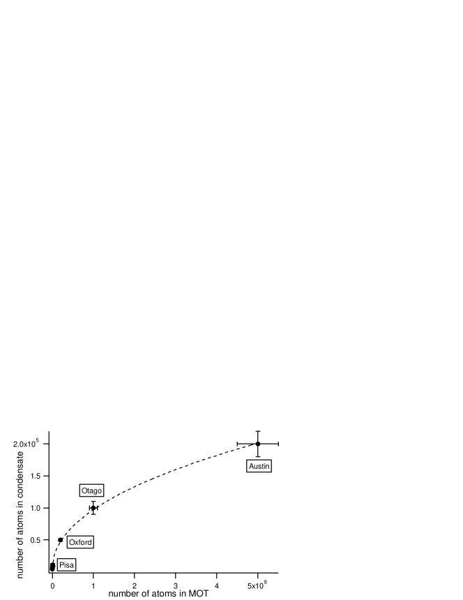
Figure 6: Typical condensate numbers of various groups as a function of initial MOT numbers. The data were taken from publications of the groups at Austin [12], Otago [14], and Oxford [15].

7 Conclusion

We have presented the results of preliminary measurements on Bose-Einstein condensates of rubidium atoms obtained in a triaxial TOP-trap. Our experimental data for the condensation threshold and the free expansion of the condensate agree well with theoretical predictions. Increasing the number of atoms in our condensates will allow us to further improve on the quality of our data and investigate the properties of the condensates in more detail.

Appendix A Anharmonic corrections in the TOP-trap

For our calibration measurements, we deduced the frequencies in the harmonic limit from the anharmonic corrections in the triaxial TOP-trap. Terms containing the amplitude of the oscillations along the $y$-axis have not been calculated as we do not excite oscillations along that direction, but can be obtained in the same manner. The expressions for the frequencies along the axis $i$ ($i=x,z$) are then

$$\nu_{i}^{\rm anh}=\nu_{i}+\Delta\nu_{i}\quad;\quad\Delta\nu_{i}=\left(\frac{b^{\prime}}{B_{0}}\right)^{2}\sum_{j}\alpha_{ij}a^{2}_{j}$$ (9)

where $\nu_{i}$ is the frequency in the harmonic approximation, as given by Eqs. 4 and $a_{j}$ is the amplitude of the oscillation in the $j$-direction. The elements $\alpha_{ij}$ of the anharmonic correction matrix are given by

$$\alpha_{xx}=\frac{\nu_{x}}{4}\left[6\frac{1-\eta^{2}}{1+\eta^{2}}\left(2-3\eta^{2}-\frac{15}{8}(1-\eta^{2})^{2}\right)-\frac{\eta^{2}(1-3\eta^{2})^{2}}{18(1+\eta^{2})}\right]$$ (10)

$$\alpha_{xz}=\frac{\nu_{x}}{4}\left[\frac{7-\eta^{2}(18-15\eta^{2})}{12}-\frac{9\eta^{2}(3\eta^{2}-1)(14+8\eta^{2})-8\eta^{2}}{36(7+9\eta^{2})}\right]$$ (11)

$$\alpha_{zx}=\frac{\nu_{z}}{2}\left[\frac{1-3\eta^{2}}{2}-\frac{2\eta^{2}(1-3\eta^{2})}{9(3+5\eta^{2})}+\frac{7-3\eta^{2}-15\eta^{2}(1-\eta^{2})}{12}\right]$$ (12)

$$\alpha_{zz}=\frac{\nu_{z}}{2}\left[-\frac{3}{8}(1-\eta^{2})(1-5\eta^{2})-\frac{15}{8}\eta^{2}(1-\eta^{2})\right].$$ (13)

References

- [1] Anderson M H, Ensher J R, Matthews M R, Wieman C E and Cornell E A 1995 Science 269 198
- [2] Bradley C C, Sackett C A, Tollett J J and Hulet R G 1995 Phys. Rev. Lett. 75 1687
- [3] Davis K B, Mewes M O, Andrews M R, van Druten N J, Durfee D S, Kurn D M and Ketterle W 1995 Phys. Rev. Lett. 75 3969
- [4] for reviews see Ketterle W, Durfee D S, and Stamper-Kurn D M, in Proceedings of Int. School “Enrico Fermi”, Course CXL, eds. Inguscio M, Stringari S, and Wieman C E, (IOS, Amsterdam 1999) pag. 67; Cornell E A, Ensher J R, and Wieman CE, in ibidem pag. 177
- [5] Dalfovo F, Giorgini S, Pitaevskii L P and Stringari S 1999 Rev. Mod. Phys. 71 463
- [6] Petrich W, Anderson M H, Ensher J R and Cornell E A 1995 Phys. Rev. Lett. 74 3353
- [7] Hagley E W, Deng L, Kozuma M, Wen J, Helmerson K, Rolston S L and Phillips W D 1999 Science 283 1706
- [8] Müller J H, Morsch O, Ciampini D, Anderlini M, Mannella R and Arimondo E 2000 to be submitted
- [9] Anderson B P and Kasevich M A 1999 Phys. Rev. A 59 R938
- [10] Castin Y and Dum R 1996 Phys. Rev. Lett. 77 5315
- [11] Ensher J R, Ph.D. Thesis 1998, University of Colorado
- [12] Han D J, Wynar R H, Courteille Ph and Heinzen D J 1998 Phys. Rev. A 57 R4114
- [13] Cornell E 2000 private communication
- [14] Martin J L, McKenzie C R, Thomas N R, Sharpe J C, Warrington D M, Manson P J, Sandle W J and Wilson A C 1999 J. Phys.B: At. Mol. Opt. Phys. 32 3065
- [15] Arlt J, Maragò O, Hodby E, Hopkins S A, Hechenblaikner G, Webster S and Foot C J 1999 J. Phys.B: At. Mol. Opt. Phys. 32 5861