Fluctuation and relaxation properties of pulled fronts:
a possible scenario for non-Kardar-Parisi-Zhang behavior

Abstract

We argue that while fluctuating fronts propagating into an unstable state should be in the standard KPZ universality class when they are pushed, they should not when they are pulled: The universal $1/t$ velocity relaxation of deterministic pulled fronts makes it unlikely that the KPZ equation is the appropriate effective long-wavelength low-frequency theory in this regime. Simulations in 2$D$ confirm the proposed scenario, and yield exponents $\beta\approx 0.29\pm 0.01$, $\zeta\approx 0.40\pm 0.02$ for fluctuating pulled fronts, instead of the KPZ values $\beta=1/3$, $\zeta=1/2$. Our value of $\beta$ is consistent with an earlier result of Riordan et al.

Over a decade ago, Kardar, Parisi and Zhang (KPZ) [1] introduced their celebrated stochastic equation

$${{\partial h}\over{\partial t}} = \nu\nabla^{2}h+{{\lambda}\over{2}}(\nabla h)^{2}+\eta~{},$$ (1)

$$\langle\eta({\bf x},t)\eta({\bf x}^{\prime},t^{\prime})\rangle = D\delta^{d}({\bf x}-{\bf x^{\prime}})\delta(t-t^{\prime})~{},$$ (2)

to describe the fluctuation properties of growing interfaces with height $h$ under the influence of the noise term $\eta$. A clear “derivation” of the KPZ equation is difficult to give, just as much as the Landau-Ginzburg-Wilson Hamiltonian can not straightforwardly be “derived” from the Ising model. However, one expects the KPZ equation to be the proper effective long wavelength low frequency theory for interfacial growth phenomena whose deterministic macroscopic evolution equation is of the form

$${{\partial h}\over{\partial t}}=v(\nabla h)+\mbox{curvature corrections}.$$ (3)

Here $v(\nabla h)$ is the deterministic growth velocity of a planar interface as a function of the orientation $\nabla h$. For, as long as the curvature corrections of the form $\nabla^{2}h$ are nonzero, the long wavelength expansion of (3) immediately yields the gradient term in (1). The philosophy is then that in the presence of noise, all the relevant terms in the KPZ equation (1) are generated, and that this is sufficient to yield the asymptotic KPZ scaling. In agreement with this picture, many interface growth models have been found [2, 3, 4, 5] to show the universal asymptotic scaling properties predicted by (1).

A dynamical interface equation of the form (3) is appropriate for interfaces whose long wavelength and slow time dynamics is essentially local in space and time, i.e., dependent on the local and instantaneous values of the slope and curvature. The applicability of the KPZ equation is therefore not limited to situations with a microscopically sharp interface: Many pattern forming systems of the reaction-diffusion type exhibit fronts whose intrinsic width $l$ is finite. For curvatures $\kappa$ small compared to $l^{-1}$, $\kappa l\ll 1$, an effective interface approximation or moving boundary approximation of the form (3) can then be derived using standard techniques [6]. These approximations apply whenever the internal stability modes of the fronts relax exponentially on a short time scale, so that an adiabatic decoupling becomes exact in the limit $\kappa l\!\rightarrow\!0$. The best known example of such a type of analysis is for the curvature driven growth in the Cahn-Hilliard equation, but moving boundary techniques have recently been applied successfully to many other such problems [6]. In all these cases, the internal relaxation modes within the fronts or transition zones are indeed exponentially decaying on a short time scale.

From the above perspective, recent results for the relaxation properties of planar fronts propagating into an unstable state, suggest an interesting new scenario for non-KPZ behavior. Fronts propagating into unstable states generally come in two classes, so-called pushed fronts and pulled fronts [7]. Pushed fronts propagating into an unstable state are the immediate analogue of fronts between two linearly stable states. In the thin interface limit, $\kappa l\ll 1$, the dynamics of such fronts becomes essentially local and instantaneous, and given by an equation of the form (3); according to the arguments given above, fluctuating pushed fronts should thus obey KPZ scaling: following standard practice by saying that the $d$+1D KPZ equation (where the +1 refers to the time dimension) describes the fluctuations of a $d$-dimensional interface, the conclusion is that fluctuations of $d$-dimensional pushed fronts in $(d$+$1)$ bulk dimensions are described by the $d$+1D KPZ equation.

Pulled fronts, however, behave very differently from pushed ones. A pulled front propagating into a linearly unstable state is basically “pulled along” by the linear growth dynamics of small perturbations spreading into the linearly unstable state. The crucial new insight for our discussion is the recent finding [7, 8] that pulled fronts can not be described by an effective interface equation like (3) that is local and instantaneous in space and time, even if they are weakly curved on the spatial scale. This just reflects the fact that the dynamically important region of pulled fronts is the semi-infinite leading edge region ahead of the front, not the nonlinear front region itself. Technically, the breakdown of an interfacial description is seen from the divergence of the solvability type integrals that arise in the derivation of a moving boundary approximation in dimensions $d$$\geq$$2$ [7]. More intuitively, the result can be understood as follows: a deterministic pulled front in $d$=$1$ relaxes to its asymptotic speed $v^{*}$ with a universal power law as $v(t)=v^{*}+c_{1}/t+c_{3/2}/t^{3/2}+\cdots$, where $c_{1}(<0)$ and $c_{3/2}$ are known coefficients [8]. Clearly, this very slow power law relaxation implies that an adiabatic decoupling of the internal front dynamics and the large scale pattern dynamics can not be made and hence that there is no long-wavelength effective interface equation of the form (3) for pulled fronts. There is then a priori no reason to expect that fluctuating pulled fronts are in the KPZ universality class!

It is our aim to test this scenario by introducing a simple stochastic lattice model whose front dynamics can be changed from pushed to pulled by tuning a single parameter. Our results are consistent with our conjecture that pulled fluctuating fronts are not in the standard KPZ universality class, while pushed fronts are. In fact, our results put an earlier empirical finding of Riordan et al. [9] into a new perspective: These authors obtained essentially the same growth exponent as we do for the non-KPZ case, but the connection with the transition from pushed to pulled front dynamics was not made.

FIG. 1.: The two versions of our stochastic model for noisy pushed and pulled fronts. The model is isotropic, i.e., all neighbors are probed with equal probability. (a) The pushed case: Stochastic moves consist of diffusive jumps of a particle to a neighboring empty site and birth and death processes at sites whose two randomly chosen nearest neighbors are occupied. (b) The pulled case: The only difference with the pushed case is in the birth and death processes.

Our stochastic model is motivated by [9] and the results for deterministic planar fronts in the nonlinear diffusion equation

$$\partial\rho/\partial t=D\nabla^{2}\rho+k_{1}\rho+k_{2}\rho^{2}-k_{3}\rho^{3}~{}.$$ (4)

As discussed in [10, 7], the planar fronts with $\rho>0$ propagating into the unstable state $\rho=0$ are pulled for all values $k_{2}<\sqrt{k_{1}k_{3}/2}$ and pushed for larger $k_{2}$. In the pulled regime, the asymptotic front velocity, is $v^{*}=2\sqrt{Dk_{1}}$, while in the pushed regime the asymptotic front velocity equals $v^{\dagger}=2\sqrt{Dk_{1}}[(-K+\sqrt{K^{2}+4})/32]$ where $K=k_{2}/\sqrt{k_{1}k_{3}}$. We confine ourselves here to studying two limits where the stochastic front dynamics can easily be understood intuitively.

We study the dynamics of particles on a square lattice, subject to the constraints that no more than one particle can occupy each lattice site. The stochastic moves are illustrated in Fig. 1. They consist of diffusive hops of particles to neighboring empty sites and of birth and death processes on sites neighboring an occupied site. In a mean field approximation, this stochastic model is equivalent to a discrete version of (4). We will study here the two cases indicated in Fig. 1. For $k_{1}=0$ (Fig. 1a), planar fronts are definitely pushed: Since the linear spreading speed $v^{*}=0$ for $k_{1}=0$, the front must then be pushed, even if corrections to the mean field behavior are important in the front region or behind the front. Likewise, when $k_{3}=0$ and $k_{2}<0$ (Fig. 1b), the nonlinearities behind the front only limit the birth (growth) rate, so in this limit the stochastic planar front is definitely pulled.

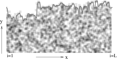
FIG. 2.: A snapshot of the coarse-grained density field ($m=1$). The interface position (continuous line) is obtained as the point where the density crosses half its bulk value.

Our simulations are done on 2D strips which are long in the $y$ direction and of width $L$ in the $x$ direction. In the $x$ direction, periodic boundary conditions are used. The Monte Carlo simulations are started with a configuration in which the first few rows ($\approx 100$) of the lattice are occupied with a probability equal to the equilibrium density. All other lattice sites are empty. After an initial transient, the scaling properties of the interface width are studied in the standard way using the following definition of the interface height $h$. We define a coarse-grained density variable at each lattice site as the average occupation of sites on a $(2m+1)\times(2m+1)$ grid centered at that site. We then define the position $h(x_{i})$ of the interface as the first point where this coarse-grained density reaches half the equilibrium density value. Our results for ensemble averaged width of the interface (see below) are obtained by averaging over $100$ runs for the largest system $L=2048$ to about $3200$ runs for the smallest $L=64$. Although we have performed simulations with $m=1,2$ and $m=3$ almost all the data presented subsequently are those for a representative value of $m=2$. The coarse-grained density field and the corresponding interface position $h$ for a typical configuration is shown in Fig. 2.

FIG. 3.: Scaling collapse of the width in the pushed (empty symbols) and the pulled (solid symbols) cases using (a) KPZ exponents $\zeta=0.5,z=1.5$ and (b) $\zeta=0.4,z=1.38$. The pushed data values are multiplied by a factor $3$ for clarity.

The interface width $w$ of a given realization is defined in the usual way, $w^{2}(t)=\overline{(h(x_{i},t)-\overline{h(x_{i},t)})^{2}}$, where the overbar denotes a spatial average, $\overline{h}=L^{-1}\sum_{x_{i}}h(x_{i},t)$. The proper scaling to study is the ensemble averaged mean square interface width $W^{2}\equiv\langle w^{2}\rangle$. As is well known, in the KPZ equation $W$ obeys a scaling form $W(t)=t^{\beta}{\cal Y}\left({{t}\over{L^{z}}}\right)$. Here the scaling function ${\cal Y}(u)$ is about constant for $u\ll 1$ and ${\cal Y}\sim u^{-\beta}$ for $u\gg 1$, with the KPZ exponents $z=3/2$ and $\beta=1/3$ in $1+1$D. For $t\gg L^{z}$, the width saturates at $W_{sat}\sim L^{\zeta}$ where $\zeta=\beta z$ is the roughness exponent. In Fig. 3, we show our data for stochastic pushed and pulled fronts by plotting $W/L^{\zeta}$ versus $t/L^{z}$ for a range of system sizes ($L=128$ to $2048$). Following standard practice, we always plot the subtracted width $W^{2}(t)-W^{2}(0)$ to minimize the effect of the initial front width. The kinetic parameters are chosen to be $k_{2}=0.5,k_{3}=1.0$ for the pushed model and $k_{2}=0,k_{1}=0.1$ for the pulled model. The diffusion rate $D=0.25$ is the same in both cases. In Fig. 3a we use the 1+1D KPZ exponents to obtain a data collapse. Clearly, good scaling collapse of the pushed data confirms that the pushed fronts are in the universality class of the 1+1D KPZ equation. By contrast, use of 1+1D KPZ values does not lead to good scaling collapse of the pulled data. In Fig. 3b we show the same sets of data but now with exponents $\zeta=0.4$ and $z=1.38$ to obtain the best possible scaling collapse of the pulled data. It is clear that the two sets of exponents, though only moderately different from each other, are well beyond error-bars. More accurate estimates of the exponents for the pulled case were obtained as follows. In Fig. 4 we fit a power law to the non-saturated part of the width for the largest system $L=2048$ and obtain $\beta\simeq 0.29\pm 0.01$ for the growth exponent. Plotting the saturated width $W_{sat}$ as a function of system size $L$ (Fig. 4, inset) yields $\zeta\simeq 0.4\pm 0.02$ for the roughness exponent. Once $\zeta$ is known the dynamic exponent is obtained by requiring good scaling collapse of Fig. 3b., $z=1.38\pm 0.06$. The value of $\beta$ is consistent with that reported by Riordan et al. [9] for this model, $\beta=0.272\pm 0.007$, but their apparent value of $z\simeq 1$ is not the true dynamic exponent related to the interface roughness through $\zeta=\beta z$, since they studied the ensemble averaged width of the front [11].

FIG. 4.: Scaling of the width in the pulled case for a system of size $L=2048$. We have taken $k_{1}=0.1,k_{2}=-1.0$ and $D=0.25$. The inset shows the saturated width $W_{sat}$ vs $L$ plot on a log-log scale for $L=64\times 2^{n}(n=0,\cdots,5)$ and is consistent with $\zeta=0.4$ (solid line).

Another way to investigate the possible difference with the 1+1D KPZ behavior is to study the distribution $P(w^{2}/W^{2})$. For 1D interface models whose long time interface configurations are given by a Gaussian distribution, like the KPZ model, the distribution function $P(w^{2}/W^{2})$ is uniquely determined, without adjustable parameters [13]. As Fig. 5 shows, in the pushed regime our data are completely consistent with this distribution function, but in the pulled regime the measured distribution function deviates significantly from the universal prediction for Gaussian interface fluctuations.

FIG. 5.: The probability distribution of the width of the interface ($x\equiv w^{2}/W^{2}$). The triangles and the circles are for the pushed and the pulled data of Fig. 3, respectively, and the solid and the dashed lines are the universal distribution functions for the $1+1$D KPZ and $2+1$D KPZ equation, as obtained by Rácz et al. [13]. Inset: the same plot on a semi-log scale showing the agreement for large arguments.

The essential difference between pushed and pulled fronts is that for pushed fronts the dynamically important region is the finite transition zone between the two phases it separates, whereas for pulled fronts it is the semi-infinite leading edge ahead of the front itself [7, 8]. It is precisely for this reason that the wandering of stochastic pulled fronts in one bulk dimension with multiplicative noise was recently found to be subdiffusive and determined by the 1+1D KPZ equation, not by a “0+1D” stochastic Langevin equation [12]. By extending this idea it has been recently conjectured [14] that the scaling exponents of stochastic pulled fronts in $d$+$1$ bulk dimensions are generally given by the $(d$$+$$1)$$+$$1$D KPZ equation instead of the $d$+1D KPZ equation, essentially because the dimension perpendicular to the front can not be integrated out [14]. The scaling exponents we find here in 2 bulk dimensions are indeed close to those reported for the $2$+$1$D KPZ equation [4], the supposedly most accurate values being $\zeta=0.393(3)$, $\beta=0.245(3)$ [15]. Moreover, the probability distribution $P(w^{2}/W^{2})$ of pulled fronts fits the $P(w^{2}/W^{2})$ of the 2+1D KPZ equation quite well without adjustable parameters, see Fig. 5. For justification and further exploration of this conjecture, we refer to [14].

An interesting limit of our model is obtained when we further take $k_{2}=0$ in Fig. 1b. In this case only birth and diffusion occurs, leading to an equilibrium density $\rho=1$ behind the front. If we put $D=0$ as well, the result is an Eden-like model [4, 5] with the modification that the probability of adding a particle is proportional to the number of neighbors, not independent of it. Numerical simulations in this Eden-like limit indicate that the KPZ exponents are recovered, as it should, and hence that the model has a KPZ to non-KPZ transition at intermediate values of $\rho_{eq}$ and $D$.

In conclusion, even though one should always be aware of the possibility of a very slow crossover to asymptotic behavior in such studies [16] — a problem that has plagued some earlier tests of KPZ scaling in, e.g., the Eden model — taken together our data as well as those of [9] give, in our opinion, reasonably convincing evidence for our scenario that the absence of an effective interface description for deterministic pulled fronts also entails non-KPZ scaling of stochastic pulled fronts.

We thank J. Krug, T. Bohr and Z. Rácz for stimulating discussions. G. Tripathy is supported by the Dutch Foundation for Fundamental Research on Matter (FOM).

REFERENCES

- [1] M. Kardar, G. Parisi and Y. C. Zhang, Phys. Rev. Lett. 56, 889 (1986).
- [2] J. Krug and H. Spohn, in Solids far from Equilibrium, C. Godrèche, ed. (CUP, Cambridge, 1992).
- [3] T. J. Halpin-Healy and Y. C. Zhang, Phys. Rep. 254, 215 (1995).
- [4] A.-L. Barabási and H. E. Stanley, Fractal Concepts in Surface Growth (CUP, Cambridge, 1995).
- [5] J. Krug, Adv. Phys. 46, 139 (1997).
- [6] See, e.g., A. Karma and W.-J. Rappel, Phys. Rev. E 57, 4323 (1998), and references therein.
- [7] U. Ebert and W. van Saarloos, Phys. Rev. Lett. 80, 1650 (1998), and condmat/0003181.
- [8] U. Ebert and W. van Saarloos Breakdown of standard Perturbation Theory and Moving Boundary Approximation for “Pulled” Fronts, condmat/0003184.
- [9] J. Riordan, C. R. Doering, and D. ben-Avraham, Phys. Rev. Lett. 75, 565 (1995).
- [10] E. Ben-Jacob, H. R. Brand, G. Dee, L. Kramer, and J. S. Langer, Physica D 14, 348 (1985).
- [11] In [9], the width is not defined relative to ; as a result, the long time data of [9] show the diffusive wandering of , rather than the saturation of .
- [12] A. Rocco, U. Ebert and W. van Saarloos, condmat/0004102, to appear in Phys. Rev. E.
- [13] G. Foltin, K. Oerding, Z. Rácz, R. L. Workman and R. K. P. Zia, Phys. Rev. E. 50, R639 (1994); Z. Rácz and M. Plischke, Phys. Rev. E 50, 3530 (1994); and Z. Rácz, unpublished.
- [14] G. Tripathy, A. Rocco, J. Casademunt and W. van Saarloos (unpublished).
- [15] E. Marinari, A. Pagnani and G. Parisi, condmat/0005105.
- [16] This might be especially true for pulled fronts, since the speed of one-dimensional fronts depends strongly on a finite-particle type cutoff. See E. Brunet and B. Derrida, Phys. Rev. E 56, 2597 (1997); D. A. Kessler, Z. Ner and L. M. Sander, Phys. Rev. E 58, 107 (1998).