IFUP-TH/2000-13 Linked-Cluster Expansion of the Ising Model

Abstract

The linked-cluster expansion technique for the high-temperature expansion of spin model is reviewed. A new algorithm for the computation of three-point and higher Green’s functions is presented. Series are computed for all components of two-point Green’s functions for a generalized $3D$ Ising model, to 25th order on the bcc lattice and to 23rd order on the sc lattice. Series for zero-momentum four-, six-, and eight-point functions are computed to 21st, 19th, and 17th order respectively on the bcc lattice.

1 Introduction

The high-temperature (strong-coupling) series expansion is one of the most successful tools for the study of physical systems near a critical point.

High-temperature series are analytic; the radius of convergence is usually quite large, often reaching the boundary of the high-temperature phase. This property allows the application of powerful techniques of resummation and analytical continuation [1], which can yield very precise and reliable results, provided that long series are available. It is therefore worthwhile to push the computation of high-temperature series as far as our algorithms and computers allow.

The most successful technique for the computation of high-temperature series of $3D$ spin models is the linked-cluster expansion (LCE), which is well suited for the fully computerized approach required to reach very high orders of the expansion.

Several detailed discussion of the LCE appeared in the literature. Wortis’ review [2] covers most of the basic topics, and provides many graphical rules fit for algorithmic implementation. Nickel performed a remarkable computation for the $3D$ Ising model on the bcc lattice [3], which had not been surpassed until the present work; in a more detailed paper, Nickel and Rehr also present several clever algorithms which we found very useful [4]. Lüscher and Weisz, describing their application of the LCE to lattice field theory, also provide several important implementation hints [5].

Unfortunately, the notation found in the literature is by no means uniform. Therefore we will review the relevant aspects of the LCE, which can be found in Ref. [2], not only to make our paper more self-contained, but also to explain notations carefully and to remark the correspondence with Refs. [2, 4, 5]. We will follow the notations of Ref. [4] whenever possible.

The paper is organized as follows:

Sect. 2 introduces the relevant graph theory concepts and definitions.

Sect. 3 presents the generalized Ising model we focus on.

Sects. 4, 5, and 6 review the LCE, with special focus on the two-point Green’s functions.

Sect. 7 describes our algorithm for the computation of three-point and higher Green’s functions.

Sect. 8 is devoted to programming details.

Sect. 9 displays a (small) selection of the series generated.

Forthcoming papers will be devoted to the analysis of the series, using the techniques presented in Ref. [6], and to the generation and analysis of the series for $XY$ systems.

We will not give proofs of our formulae. The only nontrivial step in the proofs of Sects. 5–7 is to show that the symmetry factors compensate exactly the different number of contributions that may appear on the two sides of the equations; it is typically a straightforward, if tedious, exercise in combinatorics. The proofs of Sects. 4–6 are given or sketched in Ref. [2]. The proofs of Sect. 7 are especially easy, since the symmetry factor of a 1-irreducible tree graph is always 1.

2 Graphology

In this section we introduce a number of graph theory concepts relevant for the LCE. We refer the reader to Ref. [7] for a comprehensive introduction to the subject.

A graph is a set of vertices and edges (also named links or bonds in the literature). Each edge $l$ is incident with two distinct vertices, its extrema (we do not allow the extrema to coincide); the set of extrema will be denoted by $\partial l$; we write $\partial l=\{i(l),f(l)\}$; the choice of an “initial” and a “final” vertex is arbitrary. Two vertices are adjacent if they are the extrema of the same edge. We will denote the number of vertices and edges of a graph by $v$ and $e$ respectively. We also consider arcs or oriented edges, incident out of the initial vertex $i(l)$ into the final vertex $f(l)$.

The valence $n(i)$ of a vertex $i$ is the number of edges incident with $i$.

An $r$-rooted graph is a graph with $v$ vertices, $v\geq r$: $r$ roots or external vertices and $v-r$ internal vertices. We will assign the indices $1$, …, $r$ to the roots and the indices $r+1$, …, $v$ to the internal vertices. In the drawings, roots will be denoted by open dots and internal vertices by filled dots.

Two $r$-rooted graphs are isomorphic if there exists a one-to-one correspondence $\pi$ of their internal vertices and edges such that the incidence relations are preserved, i.e., $\partial(\pi(l))=\{\pi(i(l)),\pi(f(l))\}$ ($\pi(i)=i$ for the roots). From now on, we will identify isomorphic graph, and silently assume that all sets of graphs we define contain only non-isomorphic graphs.

The symmetry factor $S({\cal G})$ of an $r$-rooted graph ${\cal G}$ is the number of isomorphisms of ${\cal G}$ into itself, i.e. the number of of permutations of internal vertices and edges preserving the incidence relations.

We will also consider $p$-ordered $r$-rooted graphs, $p\leq r$, i.e. the classes of rooted graphs isomorphic up to permutations of $r-p$ roots. We will assign indices $1$, …, $p$ to the fixed roots and indices $p+1$, …, $r$ to the roots which can be permuted. The symmetry factor $S({\cal G})$ is defined as the number of isomorphisms of ${\cal G}$ into itself, including permutation of the roots $p+1$, …, $r$. The symmetry factor divided by $(r-p)!$ is called the modified symmetry factor $S_{E}({\cal G})$ (cfr. Ref. [5]); it need not be an integer. The $r$-rooted graphs defined above are ordered ($r$-ordered); unless otherwise specified, we will assume that graphs are ordered. 0-ordered graphs are unordered.

We will also discuss ($p$-ordered) $r$-rooted graphs whose edges and/or vertices are assigned a label; let us consider e.g. the case of an edge label $a(l)$ and vertex label $b(i)$. Two labelled graphs $({\cal G},a,b)$ and $({\cal G}^{\prime},a^{\prime},b^{\prime})$ are equivalent (isomorphic) if there exists an isomorphism of ${\cal G}$ into ${\cal G}^{\prime}$ such that $a$ is mapped into $a^{\prime}$ and $b$ is mapped into $b^{\prime}$. The symmetry factor $S({\cal G},a,b)$ is the number of isomorphisms of $({\cal G},a,b)$ into itself.

A pair of vertices $i$ and $j$ is connected if there exists a sequence of vertices $k_{1}$, …, $k_{n}$, with $k_{1}=i$ and $k_{n}=j$, and a sequence of edges $l_{1}$, …, $l_{n-1}$ such that $\partial l_{a}=\{k_{a},k_{a+1}\}$, $a=1$, …, $n-1$. A graph is connected if every pair of its vertices is connected. In the following, unless otherwise noted, we will assume that every graph is connected.

A sequence of distinct vertices $k_{1}$, …, $k_{n}$ and distinct edges $l_{1}$, …, $l_{n}$ is called a loop of length $n$ if $\partial l_{a}=\{k_{a},k_{a+1}\}$, $a=1$, …, $n-1$, and $\partial l_{n}=\{k_{n},k_{1}\}$. The number of independent loops (also known as cyclomatic number) of a connected graph is $e-v+1$.

A connected graph is called a tree graph if it contains no loop. A tree graph has $v-1$ edges.

3 The model

We wish to compute the high-temperature (HT) expansion of the $q$-point functions of a generalized Ising model on a $D$-dimensional Bravais lattice $\Lambda$; notice that Bravais lattices enjoy inversion symmetry at each lattice site. The model is defined by the generating functional

$$\exp(W[h])={1\over Z}\prod_{i}\left[\int d\phi_{i}\,f(\phi_{i})\exp(h_{i}\phi_{i})\right]\exp\Biggl{(}K\sum_{\langle ij\rangle}\phi_{i}\phi_{j}\Biggr{)},$$ (1)

where $\phi_{i}$ is a scalar field, $f$ is an even non-negative function or distribution decreasing faster than $\exp(-\phi^{2})$ as $\phi\to\infty$, normalized by the condition

$$\int d\phi\,f(\phi)=1,$$

$K=\beta J$, the sum runs over all pairs of nearest neighbours, and the normalization $Z$ is fixed by requiring $W[0]=0$.

The connected $q$-point function (denoted by $\cal M$ in Ref. [2]) at zero magnetic field is defined by

$$G_{q}(x_{i_{1}},...,x_{i_{q}})\equiv\left.\langle\phi_{i_{1}}...\phi_{i_{q}}\rangle^{\rm con}\right|_{h=0}=\left.\partial^{q}W[h]\over\partial h_{i_{1}}\,...\,\partial h_{i_{q}}\right|_{h=0},$$ (2)

where $x_{i}\equiv(x_{1}(i),...,x_{D}(i))$ is the coordinate vector of the lattice site $i$. $G_{q}$ is invariant under the lattice symmetry group, including (discrete) translations, and under permutation of its arguments; it is customary to write $G_{2}(x_{i_{1}},x_{i_{2}})$ in the form $G_{2}(x_{i_{1}}-x_{i_{2}})$. We will apply the LCE to the computation of $G_{q}$.

4 Unrenormalized expansion

Let us parametrize the potential $f$ in terms of the bare vertices $\mu_{0}(2n)$, defined by the generating function

$$\exp\left[\sum_{n}{\mu_{0}(2n)\over(2n)!}\,h^{2n}\right]=\int d\phi\,f(\phi)\exp(h\phi).$$ (3)

These quantities are named bare semi-invariants and denoted by ${M_{n}}^{0}$ in Ref. [2]; they are named cumulant moments and denoted by $\mu_{2n}$ in Ref. [4]; $\mu_{0}(2n)=(2n-1)!!\,\vbox{\hbox{\hbox{}\kern 2.5pt$\scriptstyle\circ$}\hbox{$m$}}^{\rm con}_{2n}$ in the notations of Ref. [5]. Without loss of generality, we can rescale $\phi$ and $K$ to fix $\mu_{0}(2)=1$.

For a generic $r$-rooted graph ${\cal G}$, we define the bare external vertex factor

$$V_{0}^{(e)}(n_{1},...,n_{r};{\cal G})=\prod_{i=1}^{r}\mu_{0}(n(i)+n_{i}),$$ (4)

the bare internal vertex factor

$$V_{0}^{(i)}({\cal G})=\prod_{i=r+1}^{v}\mu_{0}(n(i)),$$ (5)

and the bare edge factor

$$L_{0}(x_{1},...,x_{v};{\cal G})=\prod_{l=1}^{e}[K\theta(x_{i(l)}-x_{f(l)})],$$ (6)

where $\theta(x)=\delta(\|x\|-1)$ and $\|x\|$ is the lattice distance between 0 and $x$.

It is convenient to focus on the contributions of $r$-rooted graphs to $q$-point functions. To this purpose we introduce the auxiliary $r$-point functions $X$, whose unrenormalized LCE is

$$X_{r}(x_{1},...,x_{r};n_{1},...,n_{r})=\sum_{{\cal G}\in{\cal I}^{(r,0)}}\sum_{x_{r+1},...,x_{v}}{V_{0}^{(e)}(n_{1},...,n_{r};{\cal G})\,V_{0}^{(i)}({\cal G})\,L_{0}(x_{1},...,x_{v};{\cal G})\over S({\cal G})},$$ (7)

where ${\cal I}^{(r,0)}$ is the set of all $r$-rooted connected graphs.

$X$ is invariant under simultaneous permutation of coordinates and valences:

$$X_{r}(x_{1},...,x_{r};n_{1},...,n_{r})=X_{r}(x_{\pi(1)},...,x_{\pi(r)};n_{\pi(1)},...,n_{\pi(r)}),$$

but not over independent permutation of coordinates and valences. Furthermore, $X$ is invariant over the lattice symmetry group, e.g. it is translation-invariant:

$$X_{r}(x_{1},...,x_{r};n_{1},...,n_{r})=X_{r}(x_{1}+x,...,x_{r}+x;n_{1},...,n_{r}).$$

$X_{1}(x;n)$ is independent of $x$, and it will be denoted by $X_{1}(n)$; it will also be denoted by $\mu(n)$ in its role of renormalized vertex. $X_{2}(x_{1},x_{2};n_{1},n_{2})$ only depends on the difference $x_{2}-x_{1}$, and it will be denoted by $X_{2}(x_{2}-x_{1};n_{1},n_{2})$. Since, by invariance under space inversion, $X_{2}(x;n_{1},n_{2})=X_{2}(-x;n_{1},n_{2})$, we also have $X_{2}(x;n_{1},n_{2})=X_{2}(x;n_{2},n_{1})$.

The sum over the location of internal vertices of the $\theta$ functions is by definition the (free) lattice embedding number of ${\cal G}$ with fixed roots:

$$\sum_{x_{r+1},...,x_{v}}\prod_{l=1}^{e}\theta(x_{i(l)}-x_{f(l)})=E(x_{1},...,x_{r};{\cal G}).$$ (8)

Therefore

$$X_{r}(x_{1},...,x_{r};n_{1},...,n_{r})=\sum_{{\cal G}\in{\cal I}^{(r,0)}}{V_{0}^{(e)}(n_{1},...,n_{r};{\cal G})\,V_{0}^{(i)}({\cal G})\,K^{e({\cal G})}\,E(x_{1},...,x_{q};{\cal G})\over S({\cal G})}.$$ (9)

Finally, the $q$-point functions are computed as:

$$G_{q}(x_{1},...,x_{q})=\sum_{\rm partitions}X_{r}(x_{i_{11}},...,x_{i_{r1}};u_{1},...,u_{r})\prod_{l=1}^{r}\delta_{u_{l}}(x_{i_{l1}},...,x_{i_{lu_{l}}}),$$ (10)

where the $q$-point delta function is

$$\delta_{1}(x_{1})=1,\quad\delta_{2}(x_{1},x_{2})=\delta(x_{1}-x_{2}),\quad...,\quad\delta_{q}(x_{1},...,x_{q})=\prod_{l=2}^{q}\delta(x_{1}-x_{l})$$

and $\{\{i_{11},...,i_{1u_{1}}\},...,\{i_{r1},...,i_{ru_{r}}\}\}$ is a generic partition of $\{1,...,q\}$ into $r$ sets of size $u_{1}$, …, $u_{r}$. We will call a root bearing a factor of $\delta_{u}$ a $u$-th order root.

The two-point function is simply

$$G_{2}(x)=X_{2}(x;1,1)+\delta(x)\,X_{1}(2).$$

5 Vertex-renormalized expansion

The graph ${\cal G}\backslash i$ is obtained by deleting from ${\cal G}$ the vertex $i$, i.e. by removing $i$ and all edges incident with $i$. A vertex $i$ of a rooted graph ${\cal G}$ is called an articulation point if there exist vertices of ${\cal G}\backslash i$ not connected to a root. A rooted graph is called 1-irreducible if it does not contain any articulation point.

Any $r$-rooted ($r>1$) connected graph ${\cal G}$ can be decomposed in a unique way into a 1-irreducible $r$-rooted 1-skeleton ${\cal S}$ and a 1-rooted 1-decoration for each vertex; ${\cal G}$ is reconstructed by decorating each vertex, identifying the root of its decoration with the vertex; an example is presented in Fig. 1.

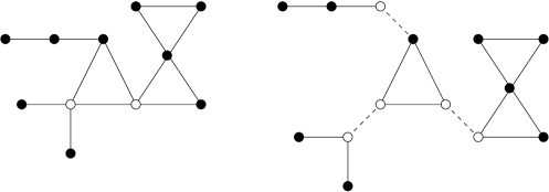
Figure 1: Example of decomposition of a graph into its 1-skeleton and 1-decorations. Open dots are roots, filled dots are internal vertices.

Since the only 1-irreducible 1-rooted graph is the single-vertex graph, we use a different definition for 1-rooted graphs. A 1-rooted graph is called a 1-skeleton if it has no articulation points except the root. Any 1-rooted connected graph ${\cal G}$ can be decomposed in a unique way into a 1-rooted 1-skeleton ${\cal S}$ and a 1-rooted 1-decoration for each vertex except the root, which is left undecorated.

A 1-rooted connected graph is called a 1-insertion if ${\cal G}\backslash 1$ is connected.

The LCE can be reorganized by summing together all contributions from graphs having the same 1-skeleton, incorporating 1-decorations into renormalized vertices $\mu(n)=X_{1}(n)$ (named semi-invariants and denoted by $M_{n}$ in Ref. [2]; $\mu(n)=(n-1)!!\,m_{n}$ in the notations of Ref. [5]). The unrenormalized LCE of $\mu(n)$ is given by Eq. (7).

The $r$-point function can be computed restricting the sum in Eq. (7) or (9) to the (much smaller) set ${\cal I}^{(r,1)}$ of 1-irreducible $r$-rooted graphs:

$$X_{r}(x_{1},...,x_{r};n_{1},...,n_{r}) = \sum_{{\cal G}\in{\cal I}^{(r,1)}}\sum_{x_{r+1},...,x_{v}}{V_{1}^{(e)}(n_{1},...,n_{r};{\cal G})\,V_{1}^{(i)}({\cal G})\,L_{0}(x_{1},...,x_{v};{\cal G})\over S({\cal G})}$$ (11)

$$= \sum_{{\cal G}\in{\cal I}^{(r,1)}}{V_{1}^{(e)}(n_{1},...,n_{r};{\cal G})\,V_{1}^{(i)}({\cal G})\,K^{e({\cal G})}\,E(x_{1},...,x_{r};{\cal G})\over S({\cal G})},$$

where the internal and external renormalized vertex factors are

$$V_{1}^{(e)}(n_{1},...,n_{r};{\cal G})=\prod_{i=1}^{r}\mu(n(i)+n_{i})$$ (12)

and

$$V_{1}^{(i)}({\cal G})=\prod_{i=r+1}^{v}\mu(n(i)).$$ (13)

Eq. (7) requires a sum over all connected graphs, and therefore it is impractical for the computation of $\mu(n)$ at large orders of the LCE. We introduce the renormalized moments $q(n)$ (named self-fields and denoted by $G_{n}$ in Ref. [2]), defined by

$$q(n)=\sum_{{\cal G}\in{\cal I}^{(1,0)}_{n,\rm in}}\sum_{x_{2},...,x_{v}}{V_{0}^{(i)}({\cal G})\,L_{0}(x_{1},...,x_{v};{\cal G})\over S({\cal G})},$$ (14)

where ${\cal I}^{(1,0)}_{n,\rm in}$ is the set of 1-insertions with root of valence $n$. The following equations hold:

$$q(n)=\sum_{{\cal G}\in{\cal I}^{(1,1)}_{n,\rm in}}\sum_{x_{2},...,x_{v}}{V_{1}^{(i)}({\cal G})\,L_{0}(x_{1},...,x_{v};{\cal G})\over S({\cal G})},$$ (15)

where ${\cal I}^{(1,1)}_{n,\rm in}={\cal I}^{(1,0)}_{n,\rm in}\cap{\cal I}^{(1,1)}$, and ${\cal I}^{(1,1)}$ is the set of 1-rooted 1-skeletons;

$$\mu(n)=\mu_{0}(n)+\sum_{s=1}^{\infty}{1\over s!}\sum_{l_{1}=1}^{\infty}...\sum_{l_{s}=1}^{\infty}q(l_{1})\,...\,q(l_{s})\,\mu_{0}(n+l_{1}+...+l_{s}).$$ (16)

Since $q(2n-1)=0$, and odd values of $n$ and $l_{i}$ do not contribute to Eq. (16). $q$ and $\mu$ can now be computed recursively in parallel order by order in $K$, since, once Eq. (15) is expanded in powers of $K$ and truncated, the coefficient of the highest power of $K$ of $q$ in the l.h.s. depends only on coefficients of lower powers of $K$ of $\mu$ in the r.h.s.

6 Edge-renormalized expansion

A pair of distinct vertices $i$ and $j$ of a rooted graph ${\cal G}$ is called an articulation pair if there exist vertices of ${\cal G}\backslash i\backslash j$ not connected to a root, or if $i$ and $j$ are joined by more than one edge. A rooted graph is called 2-irreducible if it does not contain any articulation pair.

Any 1-irreducible $r$-rooted ($r>2$) graph ${\cal G}$ can be decomposed in a unique way into a 2-irreducible $r$-rooted 2-skeleton ${\cal S}$ and a 1-irreducible 2-rooted 2-decoration for each edge (oriented in a canonical way, e.g. by choosing $i(l)<f(l)$); ${\cal G}$ is reconstructed by replacing each edge with its decoration, identifying the first and second decoration root with the initial and final vertex of the edge respectively. An example is shown in Fig. 2.

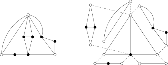
Figure 2: Example of decomposition of a graph into its 2-skeleton and 2-decorations. Open dots are roots, filled dots are internal vertices.

We use a different definition for 2-rooted graphs, since the only 2-irreducible 2-rooted graph is the bond graph (no internal vertices and only one edge); the roots of all other 1-irreducible 2-rooted graphs are an articulation pair. We call a 1-irreducible 2-rooted graph a 2-skeleton if it does not contain any articulation pair except the pair consisting of the two roots. Any 1-irreducible 2-rooted graph can be decomposed in a unique way into a 2-rooted 2-skeleton ${\cal S}$ and a 1-irreducible 2-rooted 2-decoration for each edge except edges connecting the roots, which are left undecorated.

The LCE can be reorganized by summing together all contributions from graphs having the same 2-skeleton, incorporating all 2-decorations into renormalized edges.

We start by decomposing Eq. (11) for $r>1$ into

$$W_{r}(x_{1},...,x_{r};n_{1},...,n_{r}) = \sum_{{\cal G}\in{\cal I}^{(r,1)}_{n_{1},...,n_{r}}}\sum_{x_{r+1},...,x_{v}}{V_{1}^{(i)}({\cal G})\,L_{0}(x_{1},...,x_{v};{\cal G})\over S({\cal G})},$$ (17)

$$X_{r}(x_{1},...,x_{r};n_{1},...,n_{r}) = \sum_{s_{1},...,s_{r}}\Biggl{[}\prod_{i=1}^{r}\mu(n_{i}+s_{i})\Biggr{]}W_{r}(x_{1},...,x_{r};s_{1},...,s_{r}),$$ (18)

where ${\cal I}^{(r,1)}_{n_{1},...,n_{r}}$ is the set of 1-irreducible $r$-rooted graphs with roots of valence $n_{1}$, …, $n_{r}$. $W_{r}$ enjoys the same symmetry properties of $X_{r}$. $W_{1}(x,n)$ is undefined.

$W_{r}$ can be computed by assigning an initial and a final valence $i_{l}$, $f_{l}$ to each oriented edge of a 2-rooted graph; the valence $i_{l}$ is incident with $i(l)$ and $f_{l}$ is incident with $f(l)$:

$$W_{r}(x_{1},...,x_{r};n_{1},...,n_{r})=\sum_{{\cal G}\in{\cal I}^{(r,2)}}\sum_{x_{r+1},...,x_{v};i_{1},...,i_{e},f_{1},...,f_{e}}\prod_{i=1}^{r}\delta(n_{i}-\nu_{i}(i_{1},...,i_{e},f_{1},...,f_{e};{\cal G}))\,$$

$$\quad\times\;{V_{2}^{(i)}(i_{1},...,i_{e},f_{1},...,f_{e};{\cal G})\,L_{2}(x_{1},...,x_{v};i_{1},...,i_{e},f_{1},...,f_{e};{\cal G})\over S({\cal G})},$$ (19)

where ${\cal I}^{(r,2)}$ is the set of 2-irreducible $r$-rooted graphs, $\nu_{i}$ is the sum of all the valences incident with the vertex $i$,

$$V_{2}^{(i)}(i_{1},...,i_{e},f_{1},...,f_{e};{\cal G})=\prod_{i=r+1}^{v}\mu(\nu_{i}(i_{1},...,i_{e},f_{1},...,f_{e};{\cal G})),$$ (20)

and

$$L_{2}(x_{1},...,x_{v};i_{1},...,i_{e},f_{1},...,f_{e};{\cal G})=\prod_{l=1}^{e}W_{2}(x_{i(l)}-x_{f(l)};i_{l},f_{l}).$$ (21)

For $r=2$ Eqs. (19) and (21) require a slight modification: we define ${\cal I}^{(2,2)}$ as the set of 2-rooted 2-skeletons; for edges incident with at least one root, we replace $W_{2}(x_{1}-x_{2};i,f)$ with $K\theta(x_{1}-x_{2})\delta_{i1}\delta_{f1}$.

The sum over graphs can be restricted to a subset of ${\cal I}^{(r,2)}$; we will discuss here the case $r=2$; the next Section will be devoted to the case $r\geq 3$. Let us start by classifying 1-irreducible 2-rooted graphs into several classes.

An internal vertex $i$ of a 1-irreducible 2-rooted graph ${\cal G}$ is called a nodal point if the roots of ${\cal G}\backslash i$ are not connected. A 1-irreducible 2-rooted graph is nodal (also named articulated or separable in the literature) if it contains one or more nodal points; otherwise it is non-nodal.

A 1-irreducible 2-rooted graph is simple if ${\cal G}\backslash 1\backslash 2$ is connected, and 1 is not adjacent to 2. By definition, all nodal graphs are simple. A 1-irreducible 2-rooted graph is a ladder graph if it is not simple and it is not the bond graph.

A 1-irreducible 2-rooted graph is elementary if it is both simple and non-nodal.

We have divided 1-irreducible 2-rooted graphs into four disjoint classes: bond, nodal, ladder, and elementary graphs. Let us separate the contributions to $W_{2}$ according to the four classes:

$$W_{2}(x;n_{1},n_{2})=W^{\rm bo}_{2}(x;n_{1},n_{2})+W^{\rm no}_{2}(x;n_{1},n_{2})+W^{\rm la}_{2}(x;n_{1},n_{2})+W^{\rm el}_{2}(x;n_{1},n_{2}),$$

i.e. bond, nodal, ladder, and elementary contributions respectively.

The bond contribution is trivial. Nodal contributions can be factorized into a product of non-nodal contributions:

$$W^{\rm no}_{2}(x;n_{1},n_{2})=\sum_{x_{3};i_{1},i_{2}}W^{\rm nn}_{2}(x_{3};n_{1},i_{1})\,\mu(i_{1}+i_{2})\,W^{\rm nn}_{2}(x-x_{3};i_{2},n_{2})$$

$$\;+\;\sum_{x_{3},x_{4};i_{1},i_{2},i_{3},i_{4}}W^{\rm nn}_{2}(x_{3};n_{1},i_{1})\,\mu(i_{1}+i_{2})$$

$$\quad\times\;W^{\rm nn}_{2}(x_{4}-x_{3};i_{2},i_{3})\,\mu(i_{3}+i_{4})\,W^{\rm nn}_{2}(x-x_{4};i_{4},n_{2})+...\,,$$ (22)

which can be written recursively as

$$W^{\rm no}_{2}(x;n_{1},n_{2})=\sum_{x_{3};i_{1},i_{2}}W^{\rm nn}_{2}(x_{3};n_{1},i_{1})\,\mu(i_{1}+i_{2})\,W_{2}(x-x_{3};i_{2},n_{2}).$$ (23)

Likewise, ladder contributions can be factorized into a product of non-ladder contributions:

$$W^{\rm la}_{2}(x;n_{1},n_{2})=\sum_{s=2}^{\infty}{1\over s!}\sum_{i_{1},...,i_{s},f_{1},...,f_{s}}\delta\Bigl{(}n_{1}-{\textstyle\sum_{t=1}^{s}}i_{t}\Bigr{)}\,\delta\Bigl{(}n_{2}-{\textstyle\sum_{t=1}^{s}}f_{t}\Bigr{)}\,\prod_{t=1}^{s}W^{\rm nl}_{2}(x,i_{t},f_{t}).$$ (24)

Elementary contributions can be computed by setting $r=2$ into Eq. (19), and restricting the sum to ${\cal I}^{(2,2)}_{\rm el}$, the set of elementary 2-rooted 2-skeletons. The sum can be further restricted to ${\cal I}^{(2,2)}_{0,\rm el}$, the set of unordered elementary 2-rooted 2-skeletons, provided that we replace $S({\cal G})$ with $S_{E}({\cal G})$ and we symmetrize the result:

$$W^{\rm el}_{2}(x;n_{1},n_{2})={1\over 2}\sum_{{\cal G}\in{\cal I}^{(2,2)}_{0,\rm el}}\sum_{x_{3},...,x_{v};i_{1},...,i_{e},f_{1},...,f_{e}}\prod_{l=1}^{2}\delta(n_{i}-\nu_{i}(i_{1},...,i_{e},f_{1},...,f_{e};{\cal G}))\,$$

$$\quad\times\;{V_{2}^{(i)}(i_{1},...,i_{e},f_{1},...,f_{e};{\cal G})\,L_{2}(x_{1},...,x_{v};i_{1},...,i_{e},f_{1},...,f_{e};{\cal G})\over S_{E}({\cal G})}+n_{1}\leftrightarrow n_{2}.$$ (25)

The last ingredient we need for a fully edge-renormalized expansion are the renormalized vertices $\mu(n)$; they can be computed by combining Eq. (16) with

$$q(n_{1}{+}n_{2})={n_{1}!\,n_{2}!\over(n_{1}+n_{2})!}(W^{\rm no}_{2}(0;n_{1},n_{2})+W^{\rm el}_{2}(0;n_{1},n_{2})),$$ (26)

reflecting the fact that the contributions to $q(n_{1}{+}n_{2})$ in Eq. (15) can be obtained from the contributions to $W_{2}(0;n_{1},n_{2})$ in Eq. (17) by identifying the roots of the 2-rooted graph, i.e. by suppressing the second root and reattaching all the edges incident with it to the first root, provided that the roots are not adjacent.

Expanding in powers of $K$ Eqs. (23), (24), (25), (26), and (16), we can compute $W^{\rm el}_{2}(x;n_{1},n_{2})$, $W^{\rm no}_{2}(x;n_{1},n_{2})$, $W^{\rm la}_{2}(x;n_{1},n_{2})$, $q(n)$, and $\mu(n)$ in parallel order by order in $K$. The only step which involves a summation over graphs is Eq. (25), where the sum only runs over ${\cal I}^{(2,2)}_{0,\rm el}$, a relatively small set.

7 Three-point and higher functions

A vertex (internal or external) $i$ of a 1-irreducible $r$-rooted graph ${\cal G}$ is called a nodal point if ${\cal G}\backslash i$ is not connected. By definition of 1-irreducibility, each connected component of ${\cal G}\backslash i$ must contain at least one root. A 1-irreducible $r$-rooted graph ${\cal G}$ is nodal if it contains one or more nodal points; otherwise it is non-nodal.

In the rest of this section, we will assume that every graph is 2-irreducible.

A nodal point $j$ of a 2-irreducible $r$-rooted graph ${\cal G}$ is called a tree-insertion point if at least one of the connected components of ${\cal G}\backslash j$ is a tree graph. The order $t$ of $j$ is the number of roots of ${\cal G}$ contained in all tree graph components of ${\cal G}\backslash j$, plus 1 if $j$ itself is a root. A 2-irreducible $r$-rooted graph is called compact if it contains no tree-insertion points.

Let us consider a 2-irreducible $r$-rooted graph ${\cal G}$. We generate a compact 2-irreducible graph ${\cal G}^{\prime}$, called the compact kernel of ${\cal G}$, by removing all the tree graphs attached to every tree-insertion point, and promoting all internal tree-insertion points to root. ${\cal G}$ is obtained by attaching a 2-irreducible tree graph to each root of ${\cal G}^{\prime}$. If ${\cal G}^{\prime}$ is not a tree graph (and therefore it has at least 3 roots), the decomposition is unique; otherwise, ${\cal G}$ itself is a tree graph. An example is shown in Fig. 3.

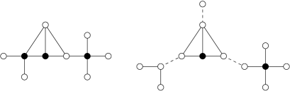
Figure 3: Decomposition of a 2-irreducible graph into a compact kernel and 2-irreducible tree graphs.

By summing all contribution of 2-irreducible graphs with the same compact kernel, we can write $W_{q}$ as

$$W_{q}(x_{1},...,x_{q};n_{1},...,n_{q})=W^{\rm tr}_{q}(x_{1},...,x_{q};n_{1},...,n_{q})$$

$$\ +\,\sum_{\textstyle{{\rm partitions}\atop r>2}}\sum_{y_{1},...,y_{r},i_{1},...,i_{r}}W^{\rm co}_{r}(y_{1},...,y_{r};i_{1},...,i_{r})\prod_{l=1}^{r}Y_{u_{l}+1}(y_{l},x_{i_{l1}},...,x_{i_{lu_{l}}};i_{l},n_{i_{l1}},...,n_{i_{lu_{l}}}),$$

(27)

where $W^{\rm tr}_{q}(x_{1},...,x_{q};n_{1},...,n_{q})$ is the tree graph contribution to $W_{q}$, $W^{\rm co}_{r}(y_{1},...,y_{r};i_{1},...,i_{r})$ is the compact graph contribution to $W_{r}$, and

$$Y_{t+1}(y,x_{1},...,x_{t};i,n_{1},...,n_{t}) = \sum_{j}\mu(i+j)\,W^{\rm tr}_{t+1}(y,x_{1},...,x_{t};j,n_{1},...,n_{t})$$

$$+ \sum_{j}\delta(y-x_{1})\,\delta(n_{1}-i-j)\,W^{\rm tr}_{t}(x_{1},...,x_{t};j,n_{2},...,n_{t}),$$

$$Y_{2}(y,x;i,n) = \sum_{j}\mu(i+j)\,W^{\rm tr}_{2}(y,x;j,n)+\delta(y-x)\,\delta(n-i)$$ (28)

(the first and second term correspond to an internal and external $t$-tree-insertion point respectively); notice that $W^{\rm tr}_{2}=W_{2}$. Eq. (27) can be combined with Eq. (10) to give

$$G_{q}(x_{1},...,x_{q})=G^{\rm tr}_{q}(x_{1},...,x_{q})$$

$$\ +\,\sum_{\textstyle{{\rm partitions}\atop r>2}}\sum_{y_{1},...,y_{r},i_{1},...,i_{r}}W^{\rm co}_{r}(y_{1},...,y_{r};i_{1},...,i_{r})\prod_{l=1}^{r}Z_{u_{l}+1}(y_{l},x_{i_{l1}},...,x_{i_{lu_{l}}};i_{l}),$$ (29)

where

$$Z_{t+1}(y,x_{1},...,x_{t};i) = \sum_{\textstyle{{\rm partitions}\atop{\rm of}\ \{1,...,t\}}}\sum_{s_{1},...,s_{r}}Y_{r+1}(y,x_{i_{11}},...,x_{i_{r1}};i,s_{1},...,s_{r})$$ (30)

$$\quad\times\ \prod_{l=1}^{r}\mu(s_{l}+u_{l})\,\delta_{u_{l}}(x_{i_{l1}},...,x_{i_{lu_{l}}}).$$

$Z_{t+1}(y,x_{1},...,x_{t};i)$ is symmetric under permutations of $x_{1},...,x_{t}$ and lattice symmetries, e.g. simultaneous translation of $y$ and $x_{1},...,x_{t}$.

These formulae can be written graphically, according to the rules presented in Table 1. A sum over all dummy coordinates $y$ and all dummy valences $i,f$ and a sum over all inequivalent permutation of external coordinates $x$ or coordinate-valence pairs $x,n$ are understood. Notice that, despite the graphical notation, all pairs of roots of $W^{\rm nn}_{q}$ and $W^{\rm co}_{q}$ are equivalent.

Table 1: Graphical rules. $\nu$ is the sum of all the valences incident with the vertex. The argument $z_{i}$ of $W^{\rm nn}_{q}$ is the coordinate $x$ or $y$ associated with the symbol placed at the vertex $i$ of the polygon; the argument $y_{i}$ of $W^{\rm co}_{q}$ is the variable $y$ of the function $Z_{q+1}$ placed at the vertex $i$.

symbol	comment	variables	factor
	internal vertex	$y$	$\mu(\nu)$
	unlabelled root	$x$, $n$	$\delta(n-\nu)$
	labelled root	$x_{1},...,x_{q}$	$\mu(q+\nu)\,\delta_{q}(x_{1},...,x_{q})$
	first root of $Z$	$x_{1},...,x_{q}$, $n$	$\mu(q+\nu+n-1)\,\delta_{q}(x_{1},...,x_{q})$
	root of $G$	$y,x_{1},...,x_{q}$	$Z_{q+1}(y,x_{1},...,x_{q};\nu)$
		$x_{1},...,x_{q}$	$G^{\rm tr}_{q}(x_{1},...,x_{q})$
		$i,f$	$W_{2}(x_{i(l)}-x_{f(l)};i,f)$
$q$-sided polygon			$W^{\rm nn}_{q}(z_{1},...,z_{q};\nu_{1},...,\nu_{q})$
$q$-sided polygon with a letter “c”			$W_{Q}$$W^{\rm co}_{q}(y_{1},...,y_{q};\nu_{1},...,\nu_{q})$

Eq. (29) can be expressed by writing all polygons with a letter “c” having 3 to $q$ vertices, placing a crossed dot with a positive integer label at each vertex in all inequivalent ways, the sum of the labels being $q$, and adding the tree contribution. The case $q=5$ is shown in Fig. 4.

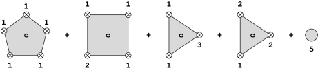
Figure 4: Graphical representation of Eq. (29) for $q=5$.

$G_{q}$ and $Z_{q}$ can be computed by adding the contributions of all 2-irreducible $r$-rooted tree graphs with roots labelled by positive integers with sum $q$; for $Z_{q}$, the first root must be drawn as a square. The case $Z_{3}$ is shown in Fig. 5.

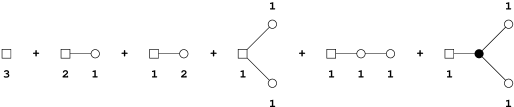
Figure 5: Contributions to $Z_{3}$.

The next step is to write an expression of $W^{\rm co}_{q}$ in terms of $W^{\rm nn}_{r}$. For $q=3$ we have simply $W^{\rm co}_{3}=W^{\rm nn}_{3}$. The case $q=4$ is shown in Fig. 6. For larger values of $q$, the number of non-nodal contributions to $W^{\rm co}_{q}$ grows rapidly, and a systematic approach is needed.

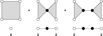
Figure 6: Compact contributions to $W^{\rm co}_{4}$ and corresponding nodal skeletons.

Let us define for a (connected or non-connected) graph ${\cal G}$ and a vertex $i$ the graph ${\cal G}/i$: let ${\cal G}^{*}$ be the connected component of ${\cal G}$ containing $i$; if ${\cal G}^{*}\backslash i$ is connected, set ${\cal G}/i={\cal G}$; otherwise, for each connected component ${\cal G}^{*}_{k}$ of ${\cal G}^{*}\backslash i$ generate the graph ${\overline{\cal G}}_{k}$ by adding a new vertex, internal or external like $i$, and joining it to all the vertices adjacent to $i$ in ${\cal G}^{*}$, by the same number of edges; replace ${\cal G}^{*}$ with the connected components ${\overline{\cal G}}_{k}$. The edges and vertices of ${\cal G}/i$ are in one-to-one correspondence with the edges and vertices of $i$, except for the new vertices which all correspond to $i$ (a nodal point of ${\cal G}$). Notice that ${\cal G}/i/j={\cal G}/j/i$.

Let ${\cal G}$ be a compact 2-irreducible $r$-rooted graph ($r\geq 3$) with $t$ nodal points $i_{1},...,i_{t}$. Observe that all the connected components ${\cal G}_{l}$ of $\overline{\cal G}\equiv{\cal G}/i_{1}/.../i_{t}$ are non-nodal. Generate a new graph ${\cal T}$, the nodal skeleton of ${\cal G}$, in the following way: for each ${\cal G}_{l}$ with $v\geq 3$, containing $n$ roots corresponding to non-nodal roots of ${\cal G}$, write a root $l$ of ${\cal T}$ with a label $n\geq 0$; for each node $i_{k}$ of ${\cal G}$ write an unlabelled vertex $i_{k}$ of ${\cal T}$, internal or external like $i_{k}$; join $i_{k}$ to all the labelled roots $l$ such that ${\cal G}_{l}$ contain a vertex corresponding to $i_{k}$, and with all unlabelled vertices which are adjacent to $i_{k}$ in ${\cal G}$.

A nodal skeleton is a connected 1-irreducible tree graph, but it is not in general 2-irreducible (it may contain 2-valent internal vertices). A nodal skeleton enjoys the following properties: each 2-valent internal vertex is adjacent to a labelled root; labelled roots are never adjacent; unlabelled roots are at least 2-valent; $m$-valent roots with label $n$ satisfy $n+m\geq 3$. Every nodal skeleton can be generated by adding labels to some of the roots and by splicing 2-valent internal vertices into a 2-irreducible tree graph.

Every 1-irreducible tree graph, with some roots carrying a non-negative integer label, satisfying the above properties, is the nodal skeleton of a set of $q$-rooted 2-irreducible compact graphs, with $q$ equal to the sum of the labels plus the number of unlabelled roots. The contribution of this set to $W^{\rm co}_{q}$ can be computed by replacing each $m$-valent root of ${\cal T}$ carrying a label $n$ with an $(n+m)$-sided polygon whose vertices are the $m$ vertices adjacent to the root and $n$ new (unlabelled) roots, and applying the rules of Table 1.

An example of the construction of the nodal skeleton and its evaluation is presented in Fig. 7. The set of all nodal skeletons contributing to $W^{\rm co}_{5}$ is shown in Fig. 8; see also Fig. 6.

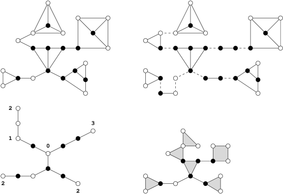
Figure 7: A compact graph, its non-nodal components, its nodal skeleton, and the contribution to $W^{\rm co}$ of the set of graphs sharing the nodal skeleton.

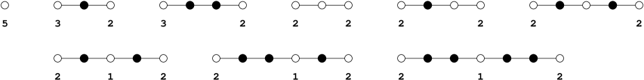
Figure 8: Nodal skeletons contributing to $W^{\rm co}_{5}$.

We could carry further the reduction of the set of graphs to be summed over, e.g. by identifying ladder graphs along the lines of Sect. 6. This is rather complicated for arbitrary $r$, and goes beyond the scope of the present work. Moreover, the zero-momentum projection described below is not applicable to the ladder graph reduction. Therefore we compute $W^{\rm nn}_{r}$ by restricting the sum of Eq. (19) to ${\cal I}^{(r,2)}_{\rm nn}$, the set of non-nodal 2-irreducible $r$-rooted graphs.

The above considerations can be simplified considerably if we are only interested in moments of the $q$-point functions, e.g.

$$\chi_{q} \equiv \sum_{x_{2},...,x_{q}}G_{q}(x_{1},...,x_{q}),$$

$$M_{2}^{(q)} \equiv \sum_{x_{2},...,x_{q}}(x_{1}-x_{2})^{2}G_{q}(x_{1},...,x_{q}).$$ (31)

Let us introduce the moments of $Z_{q}$, $W_{q}^{\rm co}$ and $W_{q}^{\rm nn}$:

$$\zeta_{q}(n) \equiv \sum_{x_{2},...,x_{q}}Z_{q}(x_{1},...,x_{q};n),$$

$$\omega^{\rm co}_{q}(n_{1},...,n_{q}) \equiv \sum_{x_{2},...,x_{q}}W^{\rm co}_{q}(x_{1},...,x_{q};n_{1},...,n_{q}),$$ (32)

the corresponding definition for $\chi^{\rm tr}_{q}$ and $\omega^{\rm nn}_{q}(n_{1},...,n_{q})$, all independent second moments, etc.

Eq. (29) can be projected over zero momentum to give

$$\chi_{q}=\chi^{\rm tr}_{q}+\sum_{r=3}^{q}\sum_{u_{1}\leq...\leq u_{r}\atop u_{1}+...+u_{r}=q}{q!\over\prod_{l=1}^{r}u_{l}!}\sum_{i_{1},...,i_{r}}\omega^{\rm co}_{r}(i_{1},...,i_{r})\prod_{l=1}^{r}\zeta_{u_{l}+1}(i_{l}).$$ (33)

The computation of $\zeta_{q}$, $\chi^{\rm tr}_{q}$, and $\omega^{\rm co}_{q}$ is also easy; the graphical rules can be immediately projected over zero momentum, suppressing all coordinates $x$ and $y$ and removing all space delta functions; the only nontrivial part is the counting of the number of inequivalent permutations of roots.

$\zeta_{q}(n)$ can be computed by summing over all inequivalent 2-irreducible 1-ordered $r$-rooted tree graphs, with the roots labelled by positive integers $u_{1},...,u_{r}$ with sum $q$. The number of inequivalent permutations of the roots 2, …, $r$ is

$${(q-1)!\over S(u_{1}-1)!\prod_{l=2}^{r}u_{l}!},$$

where $S$ is the symmetry factor of the labelled graph.

The computation of $\chi^{\rm tr}_{q}(n)$ is very similar, but we sum over unordered graphs, and the number of inequivalent permutations of the roots is

$${q!\over S\prod_{l}u_{l}!}.$$

$\omega^{\rm co}_{q}(n_{1},...,n_{q})$ can be computed by summing over all inequivalent unordered $r$-rooted nodal skeletons, with $p$ roots labelled by non-negative integers $u_{1},...,u_{p}$ with $r-p+u_{1}+...+u_{p}=q$, with a weight $1/S$, where $S$ is the symmetry factor of the labelled graph, with unlabelled roots assigned an arbitrary distinct label (e.g. $-1$).

Finally, we can compute $\omega^{\rm nn}_{q}(n_{1},...,n_{q})$ by summing over unordered non-nodal 2-irreducible $q$-rooted graphs, provided that we use the modified symmetry factor and we symmetrize the result under permutation of the valences.

The computation of the second moment of the above quantities proceeds along the same lines. The factor $(x_{i}-x_{j})^{2}$ in Eq. (31) is dealt with in the following way: the two roots are connected by a chain of terms with a space structure of the form

$$\sum_{x_{j},y_{1},...,y_{n}}(x_{i}-x_{j})^{2}f_{1}(x_{i}-y_{1})\,f_{2}(y_{1}-y_{2})\,...\,f_{n+1}(y_{n}-x_{j})$$

(we have dropped the dependency on coordinates lying outside the branch connecting $i$ with $j$). Let us write

$$(x_{i}-x_{j})^{2}=(x_{i}-y_{1})^{2}+(y_{1}-y_{2})^{2}+...+(y_{n}-x_{j})^{2}+\hbox{cross terms}.$$

The cross terms do not contribute to the sum, and the result is

$$f_{1}^{(2)}f_{2}^{(0)}...f_{n+1}^{(0)}+f_{1}^{(0)}f_{2}^{(2)}...f_{n+1}^{(0)}+...+f_{1}^{(0)}f_{2}^{(0)}...f_{n+1}^{(2)},$$

where

$$f_{i}^{(0)}=\sum_{y}f_{i}(y),\qquad f_{i}^{(2)}=\sum_{y}y^{2}f_{i}(y).$$

Therefore we can compute the second moment by taking each contribution to the zero-momentum quantity, promoting one of the zero-momentum factors along the branch connecting the roots $i$ and $j$ to second moment, and summing over all possible choices.

By dealing with moments, we avoid the need of storing all the values of $Z$, $W^{\rm co}$, and $W^{\rm nn}$, which can rapidly exhaust all available memory. The extension to higher moments is straightforward but cumbersome.

8 Programming details

We wrote a set of computer programs to implement the automatic evaluation of the edge-renormalized LCE on the simple cubic lattice (sc) and on the body-centered cubic lattice (bcc) ($3D$); the same programs evaluate the LCE on two different representations of the square lattice ($2D$) and on the $1D$ lattice.

The computation of $q$-point functions is performed for a generic potential, keeping $\mu_{0}(2n)$ symbolic; each term of the series is a polynomial in $\mu_{0}(2n)$ with rational coefficients. We also implemented the same computation for a specific potential; this requires much less memory and is somewhat faster (up to 30%), but not enough to give up the flexibility of a generic potential.

To speed up search and insertion into ordered sets of data, graph sets and polynomials in $\mu_{0}(2n)$ are implemented as AVL trees (height-balanced binary trees) (cfr. e.g. Ref. [8], Chapt. 6.2.3), using the ubiqx library. Rational numbers and (potentially) large integers are handled by the GNU multiprecision (gmp) library.

Given the complexity of the procedure, it is crucial to perform a number of checks in order to flush out all algorithm and program errors. In $1D$ our series are compared with exact results for the spin-1/2 [9] and the spin-1 [10] Ising model; this is already a very stringent check, especially of the graph sets (cfr. Ref. [4]). In $2D$, our results are compared with the series for $\chi$ and $M_{2}$ for spin-1/2 published in Ref. [3]. In $3D$, our results are compared with the lower-order series already available, for $\chi$ and $M_{2}$ for specific potentials in Refs. [3, 4, 11], and for $\chi$, $M_{2}$, and $\chi_{q}$ for a generic potential in Ref. [6]. $q(n)$ can be computed from different combinations of $n_{1}$ and $n_{2}$ in Eq. (26); their agreement is non-trivial. Finally, for the spin-1/2 Ising model on any lattice, the series for $G_{q}$, rewritten in terms of $v=\tanh K$, must have integer coefficients.

8.1 Graph generation

A program generates the table of all unordered elementary 2-rooted 2-skeletons contributing to the desired order; the algorithm follows Ref. [4]. Starting from the graph drawn in Fig. 9, we apply recursively the following modified Heap rules [12]:

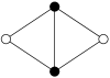
Figure 9: The simplest elementary 2-rooted 2-skeleton.

(a) join any two distinct vertices by a new edge, provided the two vertices are not already adjacent;

(b) insert a new internal vertex on any edge and join it to any vertex, excluding the edge extrema, by a new edge;

(c) insert two new internal vertices on any two distinct edges, and join them by a new edge;

(d) do not join the roots by a new edge.

The modifications to the original Heap rules (a), (b), and (c), marked in italics, prevent the generation of 2-reducible graphs. Rule (d) prevents the generation of ladder graphs.

The reduction of graphs to canonical form is performed using a generalization of the algorithm of Ref. [4]. Graphs are stored in a compact form similar to the one of Ref. [4].

To reduce the proliferation of graphs at higher orders, it is extremely important to know the order (“strict bound”) $o_{s}$ at which a given graph will enter in the expansion (it is not trivially $e$, since we require even valence of all internal vertices, and, being interested in bipartite lattices, even length of all loops).

We must also keep in mind that some graphs don’t contribute at the desired order, but graphs generated from them might contribute. We define the “Heap bound” $o_{H}({\cal G})$ as the minimum of $o_{s}$ on the set of graphs including ${\cal G}$ and all graphs generated from it. We also define the two bounds for $({\cal G},\eta)$, i.e. the minimal order when the vertex $i$ is forced to be embedded in a lattice site of parity $\eta(i)$.

We apply the modified Heap rules to the graph ${\cal G}$ in the following way: assign a parity label $\eta(i)$ to each vertex, in all the ways compatible with the Heap bound; apply the modified Heap rules assigning all possible parity labels to the new vertices; discard immediately the generated graph-parity pairs not satisfying the Heap bound; discard vertex parity information and store the generated graphs not isomorph to previously generated graphs. Finally, save into a file only the graphs satisfying the strict bound.

The generation of the elementary 2-rooted 2-skeletons contributing to the 25th order required 41 hours of computation on one CPU of a Compaq ES-40, and ca. 300 Mbytes of RAM. The number of inequivalent elementary 2-skeletons for each order of $o_{s}$ is reported in Table 2.

Table 2: Number of inequivalent unordered elementary 2-rooted 2-skeletons ($r=2$), or unordered non-nodal 2-irreducible $r$-rooted graphs ($r>2$), for each order of the strict bound $o_{s}$. The number of graphs satisfying the Heap bound is typically 20% to 30% higher. No graph in any of these sets has a bound lower than 4.

$o_{s}$	$r=2$	$r=3$	$r=4$	$r=5$	$r=6$	$r=7$	$r=8$
04	0	1	1	0	0	0	0
05	0	0	0	0	0	0	0
06	0	0	1	2	1	0	0
07	0	1	1	1	1	0	0
08	1	3	5	4	4	2	1
09	0	2	4	6	6	5	2
10	3	7	19	26	27	22	12
11	0	9	23	47	63	48	33
12	13	46	111	175	229	228	159
13	6	54	168	378	603	661	575
14	59	263	737	1436	2224	2691	2465
15	29	367	1364	3473	6404	8694	9216
16	367	1855	5824	13190	23766	34106	38239
17	197	2898	12088	34726	72900	116210	146284
18	2589	14937	51801	133739	275031
19	1547	25332	118225	375859	884317
20	21682	135325	514319
21	13933	245306	1251818
22	199865
23	139610
24	2026682
25	1516576

A similar program generates all unordered non-nodal 2-irreducible $r$-rooted graphs for $r\geq 3$. The table is initialized by applying rules (a) and (b) recursively, starting from each 2-irreducible $r$-rooted tree graph, until the result is non-nodal. Rules (a), (b), and (c) are then applied recursively. The number of inequivalent non-nodal 2-irreducible $r$-rooted graphs for each order of $o_{s}$ is reported in Table 2.

We remark that this graph tables can be used for the LCE of any spin model with $\phi\to-\phi$ symmetry on a bipartite lattice in any dimension.

The generation of all the required families of tree graphs is straightforward.

8.2 Computation of the $q$-point functions

A separate program reads the table of elementary 2-rooted 2-skeletons and computes all components of $W_{2}$.

The evaluation of $\mu$ and of bond, nodal, and ladder contribution to $W_{2}$ is a straightforward application of the formulae of Sect. 6.

The evaluation of elementary contribution dominates the computation time, and must be optimized as much as possible. Assume that all lower-order contributions to $W_{2}$ have been computed. For each unordered elementary 2-skeleton ${\cal G}$ with $o_{s}$ not larger than the desired order, all inequivalent assignations ${\cal G},(n,l)$ of edge valence parity $n$ and length parity $l$ compatible with the desired order, with even length of all loops, and with even valence of all internal vertices, are generated. We have implemented two different algorithms for the computation of the contribution of ${\cal G},(n,l)$ to the two-point function.

The first algorithm is essentially the one used by Nickel and Rehr in Ref. [4]: all inequivalent 1-irreducible 2-rooted graphs with a 2-skeleton compatible with ${\cal G},(n,l)$ are generated, and their contributions are computed according to Eq. (11). In the second algorithm, the contribution is computed according to Eq. (25), and 1-irreducible graphs are not needed. The first algorithm is more efficient for 2-skeletons with large $o_{s}$, while the second algorithm is more efficient for small $o_{s}$; for each value of $o_{s}$ we select the algorithm which is (presumably) more efficient. On the sc lattice, the speed-up obtained over the use of either algorithm for all skeletons grows with the order, and is about a factor of 4 at order 23. On the bcc lattice, the first algorithm is very efficient, since the embedding number factorizes into a product of 1-dimensional embedding numbers [4]; we still use the second algorithm for the simplest 2-skeletons ($o_{s}\leq 10$), since the computation of the corresponding 1-irreducible 2-rooted graphs contributing to orders higher than 21 is extremely time- and memory-consuming.

Keeping in RAM all components of $W_{2}$ for a generic potential would be problematic. Most of these components are needed only to compute nodal and ladder contributions, and can be kept on disk; keeping in RAM just the components needed to compute elementary contribution is manageable.

The computation of the 25th-order LCE for the two-point function on the bcc lattice required ca. 400 hours of computation, and ca. 700 Mbytes of RAM.

A similar program reads the table of non-nodal 2-irreducible $r$-rooted graphs and the components of $W_{2}$, and computes $\omega^{\rm nn}_{q}$. The computation of $\chi_{q}$ is then straightforward. We computed $\chi_{4}$, $\chi_{6}$, and $\chi_{8}$ to 21st, 19th, and 17th order respectively on the bcc lattice.

The computation of the same quantities on the sc lattice is much slower (but does not requires more RAM); so far, we obtained $W_{2}$ to 23th order, with an effort not much smaller than the 25th order on the bcc lattice. The computation of $W_{2}$ and $\chi_{q}$ to the same orders as on the bcc lattice is in progress, but it will require a non-trivial amount of time.

9 Selected results

All high-temperature series computed in the present work are available for the most general potential, in the form of polynomials in the bare vertices $\mu_{0}(2n)$. The general results are extremely lengthy, and are only useful for further computer processing.

We present here a selection of high-temperature series for the spin-1/2 Ising model, i.e. for

$$f(\phi)=\textstyle{1\over 2}\Bigl{(}\delta(\phi+1)+\delta(\phi-1)\Bigr{)}.$$

For sake of compactness, all the series are written in terms of $v=\tanh K$. Series for other specific potentials are available upon request from the author.

Although we computed all components of $G_{2}(x,y)$, we report here only $\chi\equiv\chi_{2}$ and $M_{2}\equiv M_{2}^{(2)}$ (cfr. Eq. (31)). For the $q$-point functions, we only computed $\chi_{q}$.

On the bcc lattice, we obtained

$$\chi = 1+8\,v+56\,{v^{2}}+392\,{v^{3}}+2648\,{v^{4}}+17864\,{v^{5}}+118760\,{v^{6}}+789032\,{v^{7}}$$ (34)

$$\;+\,5201048\,{v^{8}}+34268104\,{v^{9}}+224679864\,{v^{10}}+1472595144\,{v^{11}}+9619740648\,{v^{12}}$$

$$\;+\,62823141192\,{v^{13}}+409297617672\,{v^{14}}+2665987056200\,{v^{15}}+17333875251192\,{v^{16}}$$

$$\;+\,112680746646856\,{v^{17}}+731466943653464\,{v^{18}}+4747546469665832\,{v^{19}}$$

$$\;+\,30779106675700312\,{v^{20}}+199518218638233896\,{v^{21}}+1292141318087690824\,{v^{22}}$$

$$\;+\,8367300424426139624\,{v^{23}}+54141252229349325768\,{v^{24}}$$

$$\;+\,350288350314921653160\,{v^{25}}+{\rm O}(v^{26});$$

$$M_{2} = 8\,v+128\,{v^{2}}+1416\,{v^{3}}+13568\,{v^{4}}+119240\,{v^{5}}+992768\,{v^{6}}+7948840\,{v^{7}}$$ (35)

$$\;+\,61865216\,{v^{8}}+470875848\,{v^{9}}+3521954816\,{v^{10}}+25965652936\,{v^{11}}$$

$$\;+\,189180221184\,{v^{12}}+1364489291848\,{v^{13}}+9757802417152\,{v^{14}}$$

$$\;+\,69262083278152\,{v^{15}}+488463065172736\,{v^{16}}+3425131086090312\,{v^{17}}$$

$$\;+\,23896020585393152\,{v^{18}}+165958239005454632\,{v^{19}}+1147904794262960384\,{v^{20}}$$

$$\;+\,7910579661767454248\,{v^{21}}+54332551216709931904\,{v^{22}}$$

$$\;+\,372033905161237212392\,{v^{23}}+2540342425838560175616\,{v^{24}}$$

$$\;+\,17301457207110720278440\,{v^{25}}+{\rm O}(v^{26});$$

$$-\chi_{4} = 2+64\,v+1168\,{v^{2}}+16576\,{v^{3}}+201232\,{v^{4}}+2204608\,{v^{5}}+22411504\,{v^{6}}$$ (36)

$$\;+\,215447872\,{v^{7}}+1981980688\,{v^{8}}+17602809920\,{v^{9}}+151865668752\,{v^{10}}$$

$$\;+\,1278888344256\,{v^{11}}+10550227820400\,{v^{12}}+85510907958720\,{v^{13}}$$

$$\;+\,682500568307184\,{v^{14}}+5374496030148928\,{v^{15}}+41821018545214608\,{v^{16}}$$

$$\;+\,321992795063663936\,{v^{17}}+2455641803116052752\,{v^{18}}+18567879503614668736\,{v^{19}}$$

$$\;+\,139310655514229882000\,{v^{20}}+1037854026688655887552\,{v^{21}}+{\rm O}(v^{22});$$

$$\chi_{6} = 16+1088\,v+36416\,{v^{2}}+853952\,{v^{3}}+15974528\,{v^{4}}+255491264\,{v^{5}}+3638767040\,{v^{6}}$$ (37)

$$\;+\,47395195712\,{v^{7}}+574950589568\,{v^{8}}+6581949043264\,{v^{9}}+71803170318144\,{v^{10}}$$

$$\;+\,752047497945024\,{v^{11}}+7606707093034368\,{v^{12}}+74649010982738112\,{v^{13}}$$

$$\;+\,713458387977120192\,{v^{14}}+6661638582474716480\,{v^{15}}+60923519621981242752\,{v^{16}}$$

$$\;+\,546923327751320201536\,{v^{17}}+4828463182433394315584\,{v^{18}}$$

$$\;+\,41987611565592990702272\,{v^{19}}+{\rm O}(v^{20});$$

$$-\chi_{8} = 272+31744\,v+1673728\,{v^{2}}+58110976\,{v^{3}}+1538207872\,{v^{4}}+33584739328\,{v^{5}}$$

$$\;+\,634387677184\,{v^{6}}+10699575811072\,{v^{7}}+164723097021568\,{v^{8}}$$

$$\;+\,2352360935459840\,{v^{9}}+31540880634427392\,{v^{10}}+400802365468148736\,{v^{11}}$$

$$\;+\,4862781935250449280\,{v^{12}}+56665753776838026240\,{v^{13}}$$

$$\;+\,637305912177206767104\,{v^{14}}+6945658883867865975808\,{v^{15}}$$

$$\;+\,73600395257678784586368\,{v^{16}}+760476823195422275111936\,{v^{17}}+{\rm O}(v^{18}).$$

On the sc lattice, we obtained

$$\chi = 1+6\,v+30\,{v^{2}}+150\,{v^{3}}+726\,{v^{4}}+3510\,{v^{5}}+16710\,{v^{6}}+79494\,{v^{7}}+375174\,{v^{8}}$$ (39)

$$\;+\,1769686\,{v^{9}}+8306862\,{v^{10}}+38975286\,{v^{11}}+182265822\,{v^{12}}+852063558\,{v^{13}}$$

$$\;+\,3973784886\,{v^{14}}+18527532310\,{v^{15}}+86228667894\,{v^{16}}+401225368086\,{v^{17}}$$

$$\;+\,1864308847838\,{v^{18}}+8660961643254\,{v^{19}}+40190947325670\,{v^{20}}$$

$$\;+\,186475398518726\,{v^{21}}+864404776466406\,{v^{22}}+4006394107568934\,{v^{23}}$$

$$\;+\,{\rm O}(v^{24});$$

$$M_{2} = 6\,v+72\,{v^{2}}+582\,{v^{3}}+4032\,{v^{4}}+25542\,{v^{5}}+153000\,{v^{6}}+880422\,{v^{7}}+4920576\,{v^{8}}$$ (40)

$$\;+\,26879670\,{v^{9}}+144230088\,{v^{10}}+762587910\,{v^{11}}+3983525952\,{v^{12}}+20595680694\,{v^{13}}$$

$$\;+\,105558845736\,{v^{14}}+536926539990\,{v^{15}}+2713148048256\,{v^{16}}+13630071574614\,{v^{17}}$$

$$\;+\,68121779384520\,{v^{18}}+338895833104998\,{v^{19}}+1678998083744448\,{v^{20}}$$

$$\;+\,8287136476787862\,{v^{21}}+40764741656730408\,{v^{22}}+199901334823355526\,{v^{23}}$$

$$\;+\,{\rm O}(v^{24}).$$

Acknowledgments

We would like to thank Michele Caselle and Ettore Vicari for many useful discussions. Special thanks are due to Paolo Rossi, who worked out exact results for the $1D$ spin-1 Ising model, and to Andrea Pelissetto, for his critical reading of the manuscript.

References

- [1] A. J. Guttmann, in Phase Transitions and Critical Phenomena, vol. 13, C. Domb and J. Lebowitz eds. (Academic Press, New York, 1989), p. 1.
- [2] M. Wortis, in Phase Transitions and Critical Phenomena, vol. 3, C. Domb and M. S. Green eds. (Academic Press, London, 1974), p. 113.
- [3] B. G. Nickel, in Phase Transitions, Cargèse 1980, M. Levy, J. C. Le Guillou, and J. Zinn-Justin eds. (Plenum, NY, 1982), p. 291.
- [4] B. G. Nickel and J. J. Rehr, J. Stat. Phys. 61, 1 (1990).
- [5] M. Lüscher and P. Weisz, Nucl. Phys. B300, 325 (1988).
- [6] M. Campostrini, A. Pelissetto, P. Rossi, and E. Vicari, Phys. Rev. E60, 3526 (1999).
- [7] J. W. Essam and M. E. Fisher, Rev. Mod. Phys. 42, 272 (1970).
- [8] D. E. Knuth, The art of computer programming, vol. 3 (Addison-Wesley publishing co., Reading, 1973).
- [9] M. Campostrini, A. Pelissetto, P. Rossi, and E. Vicari, Nucl. Phys. B459, 207 (1996).
- [10] P. Rossi, private communication.
- [11] P. Butera and M. Comi, Phys. Rev. B56, 8212 (1997).
- [12] B. R. Heap, J. Math. Phys. 7, 1582 (1966).