Ab-initio prediction of the electronic and optical excitations in polythiophene: isolated chains versus bulk polymer

Abstract

We calculate the electronic and optical excitations of polythiophene using the $GW$ approximation for the electronic self-energy, and include excitonic effects by solving the electron-hole Bethe-Salpeter equation. Two different situations are studied: excitations on isolated chains and excitations on chains in crystalline polythiophene. The dielectric tensor for the crystalline situation is obtained by modeling the polymer chains as polarizable line objects, with a long-wavelength polarizability tensor obtained from the ab-initio polarizability function of the isolated chain. With this model dielectric tensor we construct a screened interaction for the crystalline case, including both intra- and interchain screening. In the crystalline situation both the quasi-particle band gap and the exciton binding energies are drastically reduced in comparison with the isolated chain. However, the optical gap is hardly affected. We expect this result to be relevant for conjugated polymers in general.

()

I Introduction

Semiconducting conjugated organic polymers have received increasing interest in recent years, especially since the discovery of electroluminescence [1] of these materials. The charge carriers and excitations in these materials have been studied extensively both experimentally and theoretically, but many important fundamental issues still remain unsolved. For instance, the magnitude of the exciton binding energy in these materials is still disputed.[2] This is a very important quantity, since e.g. in photovoltaic devices (solar cells) one would like to have a small binding energy, which facilitates the fast separation of charges, while in electroluminescent devices such as LEDs a larger exciton binding energy, to increase the probability of fast (radiative) annihilation of electron-hole pairs, is desirable.

In conventional semiconductors such as Si and GaAs the optical excitations are well described in terms of very weakly bound electron-hole pairs (so-called Wannier excitons) with a binding energy of the order of 0.01 eV. In crystals made of small organic molecules such as anthracene, the exciton is essentially confined to a single molecule (Frenkel exciton), leading to a binding energy of the order of 1 eV. The question is where exactly conjugated polymers fit in between conventional semiconductors on the one hand and molecular crystals on the other: negligibly small (0.1 eV or less [3]), intermediate ($\sim$ 0.5 eV [4]), and large ($\sim$ 1.0 eV [5, 6, 7]) binding energies have been proposed.

Ab-initio calculations, on a variety of conjugated polymers, within the Local Density Approximation of Density Functional Theory (DFT-LDA) yield equilibrium structures in very good agreement with experiment.[8, 9, 10, 11] The Kohn-Sham gaps in these calculations are typically 40% smaller than the optical band gap (absorption gap). In cases where calculations for both isolated chains and the crystalline situation were performed, small differences (0.1 to 0.2 eV for gaps of $\sim 3.0$ eV) in Kohn-Sham band gaps were found.[10, 11] However, it is well known that the Kohn-Sham eigenvalues formally cannot be interpreted as excited state energies.[12] Moreover, excitonic effects are not taken into account in these calculations.

An ab-initio many-body calculation within the $GW$ Approximation [13] ($GW$A) was performed for poly-acetylene (PA) by Ethridge et al.[14] They claim that their quasi-particle (QP) gap, excluding excitonic effects, is in agreement with the experimental absorption gap. This result seems to be in contrast with a more recent calculation by Rohlfing and Louie [15] of both one- (QP) and two-particle (exciton) excitation energies for PA and poly-phenylene-vinylene (PPV) chains. Their absorption gaps are in good agreement with experiments, but the inclusion of excitonic effects proves to be crucial for this. However, their exciton binding energy of 0.9 eV for PPV is much larger than recently obtained experimental values: $0.35\pm 0.15$ eV for an alkoxy-substituted PPV, [4] and $0.48\pm 0.14$ eV[16] for unsubstituted PPV.

In a recent Letter, [17] hereafter referred to as I, we focused on the differences in excitations between an isolated polythiophene (PT) chain, see Fig. 1, and crystalline polythiophene. For the isolated chain, we found an absorption gap in good agreement with experiment, but the energy differences between the various exciton levels were too large. [18] After including the screening by the surrounding chains, both the optical gap and the exciton transition energies were in good agreement with the experimental values. The difference in screening between an isolated polymer chain and a condensed polymer medium can be explained as follows. For an isolated quasi-one dimensional system, such as a single polymer chain in vacuum, there is no long-range screening. [19, 20, 21] A way to understand this is to realize that if we have two charges on a polymer chain with a separation larger than the width of the chain ($\sim 7$ a.u.), most field lines connecting the charges will be outside the chain. If the chain is embedded in a medium (possibly, but not necessarily, consisting of similar chains), the medium will provide a long-range screening of the Coulomb interaction. The screened Coulomb interaction determines both the QP energies (including the band gap) and the exciton energies. Long-range screening reduces both the QP band gap and the exciton binding energies. Apparently, there is a near cancellation between the change of the QP gap and the exciton binding energy, meaning that the optical absorption gap, which is the difference between the two, is influenced much less by introducing screening.

In I, a method for the calculation of the dielectric tensor of crystalline polythiophene from the ab-initio single chain polarizability function was introduced, without giving any details. Further, some novel technical procedures in the $GW$A calculation were used, in particular in the handling of the Coulomb divergence both in real and reciprocal space. Details of these approaches, as well as of the calculation of the quasi-particle energies and exciton binding energies, will be explained here. The paper is organized as follows: in the next section (II) we explain the computational methods employed to calculate the quasi-particle bandstructure, to regularize Coulomb interaction, to calculate the exciton binding energies and the dielectric tensor. In Section III, we will present results for the electronic and optical excitations of both the isolated chain and bulk PT. In section IV we will discuss these results and compare them to other calculations, and draw our conclusions.

II Computational methods

Many successful ab-initio calculations of the QP band structure of conventional anorganic semiconductors have been performed within the $GW$A [13] for the electronic self-energy $\Sigma$ of the one-particle Green function. Very recently, progress has been made in the evaluation of the two-particle Green function, [22, 23, 24] from which the optical properties can be obtained. This is done by solving the Bethe-Salpeter equation[25, 26] (BSE), which can be mapped onto a two-body Schrödinger equation for an electron and a hole forming an exciton. We will use these approaches to calculate the QP band structure and exciton binding energies of PT. The calculational scheme is as follows: first we perform a DFT-LDA-based Car-Parrinello calculation, from which we obtain atomic positions, wave functions and ground-state energies. We use these as input for the $GW$A calculation, which yields the QP excitation energies. With the DFT-LDA wave functions and the QP energies we calculate the two-particle excitations by solving the BSE. This scheme is first applied to the single chain and next to the crystal. We assume the same atomic geometry for the ground and excited states, i.e. the coupling between electronic and lattice degrees of freedom is neglected. Experimental data [18] indicate that energy shifts due to lattice relaxations are of the order of 0.1 eV in PT. DFT-LDA calculations [27] predict a hole-polaron relaxation energy of 0.04 eV for 16T ($n$T is an oligomer consisting of $n$ thiophene-rings). A similar calculation predicts a triplet exciton relaxation energy of 0.2 eV for 12T. [28] Singlet relaxation energies are typically smaller. These values, calculated for oligomers, are upper bounds for the values in the polymer, since in the oligomers the excitation is confined, leading to a larger local deviation from the ground state density and hence to a larger relaxation energy than in the polymer.

A The quasi-particle equation

We start our calculations with a pseudo-potential plane-wave DFT-LDA calculation [9] of a geometry-relaxed PT chain in a tetragonal supercell. The plane wave cut-off energy is 40 Ry. The length in the chain direction $a_{x}$ was optimized and found to be $a_{x}=14.80$ a.u. (experimental values range from $14.65$ a.u.[29] to $15.18$ a.u.[30]). In the perpendicular directions we found that a separation of $a_{y}=a_{z}=15.0$ a.u. is enough to consider the chains in the DFT-LDA calculation as non-interacting. The two rings in the unit cell are found to be co-planar and we choose them in the $y=z$ plane. We use Hartree atomic units (with the Bohr radius $a_{0}$ as unit of length and the Hartree as unit of energy) throughout this article, unless specified otherwise. The one-particle excitation energies are evaluated by solving the QP equation:

$$\left[-\frac{\nabla^{2}}{2}+V_{H}(\mbox{\bf{r}})\right]\phi_{nk}(\mbox{\bf{r}})+\int\left[V_{PP}(\mbox{\bf{r}},\mbox{\bf{r}}^{\prime})+\Sigma(\mbox{\bf{r}},\mbox{\bf{r}}^{\prime},E_{nk})\right]\phi_{nk}(\mbox{\bf{r}}^{\prime})d^{3}r^{\prime}=E_{nk}\phi_{nk}(\mbox{\bf{r}}),$$ (1)

where $V_{H}$ is the Hartree potential, $V_{PP}$ the non-local pseudo-potential of the atomic core, and $\Sigma$ the electronic self-energy. Since in practice the DFT-LDA wave functions and the QP wave functions are almost identical, we use the former in all calculations. In DFT-LDA, $\Sigma$ is approximated by:

$$\Sigma(\mbox{\bf{r}},\mbox{\bf{r}}^{\prime},\omega)=V_{xc}(\mbox{\bf{r}})\delta(\mbox{\bf{r}}-\mbox{\bf{r}}^{\prime}),$$ (2)

where $V_{xc}$ is the exchange-correlation potential of the homogeneous electron gas. In the $GW$A, $\Sigma$ is approximated by the first term of the many-body expansion in terms of the one-particle Green function $G$ and the screened Coulomb interaction $W$ of the system.[13] In order to calculate $\Sigma$, we follow the real-space imaginary-time formulation of the $GW$A of Rojas et al.,[31] in its mixed-space formulation. [32] In this formulation, we transform non-local functions $F(\mbox{\bf{r}},\mbox{\bf{r}}^{\prime})$ to functions $F_{k}(\mbox{\bf{r}},\mbox{\bf{r}}^{\prime})$

$$F_{k}(\mbox{\bf{r}},\mbox{\bf{r}}^{\prime}) = \sum_{n=1}^{n_{k}}F(\mbox{\bf{r}}+na_{x}\hat{x},\mbox{\bf{r}}^{\prime})e^{-ik(x+na_{x}-x^{\prime})},$$ (3)

$$F(\mbox{\bf{r}},\mbox{\bf{r}}^{\prime}) = \frac{1}{n_{k}}\sum_{k}F_{k}(\mbox{\bf{r}},\mbox{\bf{r}}^{\prime})e^{ik(x-x^{\prime})},$$ (4)

where $n_{k}$ is the number of equidistant $k$-points in the 1D Brillouin zone (BZ). We use periodic boundary conditions: $F(\mbox{\bf{r}}+n_{k}a_{x}\hat{x},\mbox{\bf{r}}^{\prime})=F(\mbox{\bf{r}},\mbox{\bf{r}}^{\prime}+n_{k}a_{x}\hat{x})=F(\mbox{\bf{r}},\mbox{\bf{r}}^{\prime})$. The functions $F_{k}(\mbox{\bf{r}},\mbox{\bf{r}}^{\prime})$ are fully periodic: $F_{k}(\mbox{\bf{r}}+a_{x}\hat{x},\mbox{\bf{r}}^{\prime})=F_{k}(\mbox{\bf{r}},\mbox{\bf{r}}^{\prime}+a_{x}\hat{x})=F_{k}(\mbox{\bf{r}},\mbox{\bf{r}}^{\prime})$, so that r and $\mbox{\bf{r}}^{\prime}$ can be chosen in the unit cell. We calculate the one-particle Green function for imaginary times

$$G_{k}(\mbox{\bf{r}},\mbox{\bf{r}}^{\prime},i\tau)=\left\{\begin{array}[]{rll}\!\!i\!\!&\displaystyle\sum_{v}u_{vk}(\mbox{\bf{r}})u^{*}_{vk}(\mbox{\bf{r}}^{\prime})e^{-(\epsilon_{vk}-\epsilon_{F})\tau}&\mbox{ for }\tau<0,\\ &&\\ \!\!-i\!\!&\displaystyle\sum_{c}u_{ck}(\mbox{\bf{r}})u^{*}_{ck}(\mbox{\bf{r}}^{\prime})e^{-(\epsilon_{ck}-\epsilon_{F})\tau}&\mbox{ for }\tau>0,\end{array}\right.$$ (5)

where $u_{nk}(\mbox{\bf{r}})=\phi_{nk}(\mbox{\bf{r}})e^{-ikx}$ and $\epsilon_{nk}$ (with $n=c,v$) are DFT-LDA wavefunctions and the corresponding energies (with $v$ and $c$ referring to valence and conduction states, respectively). $\epsilon_{F}$ is the Fermi energy (set in the middle of the DFT-LDA gap). We further calculate the irreducible single-chain polarizability function in the Random Phase Approximation (RPA)

$$P_{k}(\mbox{\bf{r}},\mbox{\bf{r}}^{\prime},i\tau)=-2i\sum_{q}G_{q}(\mbox{\bf{r}},\mbox{\bf{r}}^{\prime},i\tau)G_{q-k}(\mbox{\bf{r}}^{\prime},\mbox{\bf{r}},-i\tau),$$ (6)

the screened Coulomb interaction

$$W_{k}(\mbox{\bf{r}},\mbox{\bf{r}}^{\prime},i\omega)=\left[\tilde{v}^{-1}_{k}(\mbox{\bf{r}},\mbox{\bf{r}}^{\prime})-P_{k}(\mbox{\bf{r}},\mbox{\bf{r}}^{\prime},i\omega)\right]^{-1},$$ (7)

where $\tilde{v}_{k}(\mbox{\bf{r}},\mbox{\bf{r}}^{\prime})$ is a cut-off Coulomb interaction in mixed space, discussed in the next Section, and we calculate the electronic self-energy

$$\Sigma_{k}(\mbox{\bf{r}},\mbox{\bf{r}}^{\prime},i\tau)=i\sum_{q}G_{q}(\mbox{\bf{r}},\mbox{\bf{r}}^{\prime},i\tau)W_{k-q}(\mbox{\bf{r}},\mbox{\bf{r}}^{\prime},i\tau).$$ (8)

We calculate all the above two-point functions on a double $24\times 24\times 24$ real-space grid for r and $\mbox{\bf{r}}^{\prime}$ in the unit cell. This corresponds to a plane wave cut-off of 25 Ry. The total number of valence and conduction bands taken into account was 300. In Eqs. (6), (7) and (8) we switch between time- and frequency domain using Fourier transforms. Our imaginary-time grid has an exponential spacing (0.25 a.u. near $\tau=0$, up to a spacing 6 a.u. near $\tau_{max}=32.0{\rm{\mbox{ }a.u.}}$) and we interpolate to a linear grid when using the Fast Fourier Transform (FFT) to imaginary frequency. A similar exponential grid is used for the imaginary frequency. We split the self-energy in an exchange part $\Sigma^{x}$ and a correlation part $\Sigma^{c}$:

$$\Sigma^{x}_{k}(\mbox{\bf{r}},\mbox{\bf{r}}^{\prime}) = \sum_{q}iG_{q}(\mbox{\bf{r}},\mbox{\bf{r}}^{\prime},-i\delta)\tilde{v}_{q-k}(\mbox{\bf{r}}^{\prime},\mbox{\bf{r}}),$$ (9)

$$\Sigma^{c}_{k}(\mbox{\bf{r}},\mbox{\bf{r}}^{\prime},i\tau) = \sum_{q}iG_{q}(\mbox{\bf{r}},\mbox{\bf{r}}^{\prime},i\tau)W^{\rm{scr}}_{q-k}(\mbox{\bf{r}},\mbox{\bf{r}},i\tau),$$ (10)

where $\delta$ is an infinitesimally small positive time, and $W^{\rm{scr}}$ is the screening interaction:

$$W^{\rm{scr}}_{k}(\mbox{\bf{r}},\mbox{\bf{r}}^{\prime},i\omega)\equiv W_{k}(\mbox{\bf{r}},\mbox{\bf{r}}^{\prime},i\omega)-\tilde{v}_{k}(\mbox{\bf{r}},\mbox{\bf{r}}^{\prime}).$$ (11)

In the calculation of $\Sigma^{x}$ we use a 1D Brillouin-zone sampling of 10 equally spaced $k$-points, and in the calculation of $\Sigma^{c}$ 4 $k$-points (since the screening interaction is short-ranged, the convergence of $\Sigma^{c}$ with respect to the number of $k$-points is faster than that of $\Sigma^{x}$). With the above parameters, the calculated QP gap has converged to within about 0.05 eV. From a two-pole fit on the imaginary-frequency axis an analytical continuation to the real-frequency axis is obtained: $\Sigma^{c}(i\omega)\rightarrow{\Sigma}^{c}(\omega)$.[31] Subsequently, the QP equation Eq. (1) can be solved by replacing the QP wave functions by the DFT-LDA wave functions and obtaining $E_{nk}$ iteratively:

$$E_{nk}=\epsilon_{nk}+\left<\phi_{nk}\left|\Sigma^{c}_{k}(E_{nk})+\Sigma^{x}_{k}-V^{xc}\right|\phi_{nk}\right>.$$ (12)

B Treatment of the Coulomb interaction

We have developed a novel procedure to deal with the $\mbox{\bf{k}}=0$ and $\mbox{\bf{r}}=\mbox{\bf{r}}^{\prime}$ singularities of the Coulomb interaction $v_{\mathbf{k}}(\mbox{\bf{r}},\mbox{\bf{r}}^{\prime})$. We will first describe the procedure for a 3D system and later explain the specific adaptations of this procedure we used for our quasi-1D system.

In reciprocal space the Coulomb interaction is given by:

$$v_{\mathbf{k}}(\mbox{\bf{K}},\mbox{\bf{K}}^{\prime})=\frac{4\pi}{|{\mathbf{k}}+{\mathbf{K}}|^{2}}\delta_{\mathbf{K},\mathbf{K}^{\prime}}.$$ (13)

We replace $v_{0}(0,0)$, which would be infinite in Eq. (13) by a finite value, which is obtained in the following way. We evaluate the integral over all space of the Coulomb interaction multiplied by a Gaussian:

$$I_{\alpha} = \int d^{3}\mbox{\bf{q}}\frac{4\pi}{q^{2}}e^{-\alpha q^{2}}=8\pi^{2}\sqrt{\frac{\pi}{\alpha}},$$ (14)

and evaluate the corresponding sum, excluding the singularity for ${\mathbf{K}}=\mbox{\bf{k}}=0$:

$$S_{\alpha}=\Delta V\sum_{{\mathbf{k},\mathbf{K}}}\mbox{}\!^{\prime}v_{\mathbf{k}}(\mbox{\bf{K}},\mbox{\bf{K}})e^{-\alpha|{\mathbf{k}}+{\mathbf{K}}|^{2}},$$ (15)

where $\mbox{\bf{k}}\in$ 1BZ, the first Brillouin zone of the 3D lattice. $\Delta V$ is the volume per $(\mbox{\bf{k}},\mbox{\bf{K}})$-point and the prime indicates that $\mbox{\bf{k}}=\mbox{\bf{K}}=0$ is excluded in this sum. We now put:

$$v_{{\mathbf{k}}=0}({\mathbf{K}}=0,{\mathbf{K}}^{\prime}=0)\equiv\lim_{\alpha\rightarrow 0}\left[I_{\alpha}-S_{\alpha}\right].$$ (16)

Finally, we obtain $v(\mbox{\bf{r}}-\mbox{\bf{r}}^{\prime})$ by a discrete FFT of $v_{\mathbf{k}}(\mbox{\bf{K}},\mbox{\bf{K}}^{\prime})$ to real space. We find a finite value for $v(\mbox{\bf{r}}-\mbox{\bf{r}}^{\prime}=0)$, solving at the same time the problem with the Coulomb singularity for $\mbox{\bf{r}}-\mbox{\bf{r}}^{\prime}=0$. In the original formulation of the space-time method,[31] the authors used a grid for $\mbox{\bf{r}}^{\prime}$ offset with respect the r-grid in order to avoid this singularity.

In order to study a truly isolated chain, which is a quasi-1D system, we have to avoid ‘crosstalk’ between periodic images of the chain in the perpendicular directions. We do this by dividing space into regions of points that are closer to the atoms of a specific chain than to those of any other. Subsequently, we cut off the Coulomb interaction $v(\mbox{\bf{r}}-\mbox{\bf{r}}^{\prime})$, obtained in the way described above, by setting it zero if r and $\mbox{\bf{r}}^{\prime}$ belong to different regions. Thus we obtain an interaction $\tilde{v}(\mbox{\bf{r}},\mbox{\bf{r}}^{\prime})$. In the construction of the Coulomb interaction $v(\mbox{\bf{r}}-\mbox{\bf{r}}^{\prime})$, we take a regular grid of k-points with a spacing in the $y$- and $z$-direction approximately equal to that in the $x$-direction. From the cut-off interaction $\tilde{v}(\mbox{\bf{r}},\mbox{\bf{r}}^{\prime})$ we obtain $\tilde{v}_{k}(\mbox{\bf{r}},\mbox{\bf{r}}^{\prime})$ in mixed space from Eq. (3) with $k$ now in the 1D Brillouin zone.

C The Bethe-Salpeter equation

The two-body electron-hole Schrödinger equation related to the BSE is solved by expanding the exciton wave functions $\Phi(\mbox{\bf{r}}_{e},\mbox{\bf{r}}_{h})$ in products of conduction $\phi_{ck}(\mbox{\bf{r}}_{e})$ and valence wave functions $\phi_{vk}(\mbox{\bf{r}}_{h})$:[22, 23, 24, 25, 26]

$$\Phi(\mbox{\bf{r}}_{e},\mbox{\bf{r}}_{h})=\sum_{k,c,v}A_{kcv}\phi_{ck}(\mbox{\bf{r}}_{e})\phi^{*}_{vk}(\mbox{\bf{r}}_{h}).$$ (17)

Here we have restricted our discussion to excitons which have zero total momentum, since only these are optically active. As we are interested in the lowest lying excitons, an expansion in the highest occupied valence ($\pi$) and lowest unoccupied conduction ($\pi^{*}$) bands is sufficient to converge the exciton energies to within 0.1 eV; energy differences are converged even better. Below, we will give all energies in eV with a precision of two decimal places. The exciton binding energies $E_{b}$ follow from the Schrödinger-like equation:[22, 23, 24]

$$[E_{ck}-E_{vk}-E_{g}+E_{b}]A_{kcv}+\sum_{k^{\prime}c^{\prime}v^{\prime}}[2V^{x}_{kcv,k^{\prime}c^{\prime}v^{\prime}}\delta_{s,0}-W_{kcv,k^{\prime}c^{\prime}v^{\prime}}]A_{{k^{\prime}c^{\prime}v^{\prime}}}=0,$$ (18)

where $E_{g}$ is the QP band gap, $E_{b}$ the exciton binding energy and $W_{kcv,k^{\prime}c^{\prime}v^{\prime}}$ are the matrix elements of the static ($\omega=0$) screened interaction

$$W_{kcv,k^{\prime}c^{\prime}v^{\prime}}=\int\!d^{3}\mbox{\bf{r}}\int\!d^{3}\mbox{\bf{r}}^{\prime}\phi_{vk}(\mbox{\bf{r}}^{\prime})\phi_{ck}^{*}(\mbox{\bf{r}})W(\mbox{\bf{r}},\mbox{\bf{r}}^{\prime},\omega=0)\phi_{v^{\prime}k^{\prime}}^{*}(\mbox{\bf{r}}^{\prime})\phi_{c^{\prime}k^{\prime}}(\mbox{\bf{r}}),$$ (19)

and $V^{x}_{kcv,k^{\prime}c^{\prime}v^{\prime}}$ the exchange matrix elements (present for singlet excitons, $s=0$, only) of the bare Coulomb interaction:

$$V_{kcv,k^{\prime}c^{\prime}v^{\prime}}^{x}=\int\!d^{3}\mbox{\bf{r}}\int\!d^{3}\mbox{\bf{r}}^{\prime}\phi_{v^{\prime}k^{\prime}}^{*}(\mbox{\bf{r}})\phi_{ck}^{*}(\mbox{\bf{r}}^{\prime})\tilde{v}(\mbox{\bf{r}},\mbox{\bf{r}}^{\prime})\phi_{vk}(\mbox{\bf{r}}^{\prime})\phi_{c^{\prime}k^{\prime}}(\mbox{\bf{r}}).$$ (20)

The integrals over space in Eqs. (19) and (20) are in the calculations replaced by summations over our real-space grid. We use wave functions and energies on a grid of 8 $k$-points and extrapolate to a grid of 100 $k$-points.

Formally, dynamical screening effects may only be ignored in the BSE if $E_{g}\gg E_{b}$. However, since it has been shown that dynamical effects in the electron-hole screening and in the one-particle Green function largely cancel each other,[33] this approximation is nevertheless valid, even if the relation $E_{g}\gg E_{b}$ does not strictly hold.

We calculate an approximate exciton size $a_{\rm{ex}}$ by fitting the exciton coefficients $A_{kcv}$ to the hydrogen-like form:

$$A_{kcv}=\frac{A_{k=0,cv}}{(1+a^{2}_{\rm{ex}}k^{2})^{2}}.$$ (21)

Note that in fact the exciton is highly anisotropic. Nevertheless, Eq. (21) gives pretty good fits and can be used to get a qualitative impression of the (relative) size of the excitons.

D Inclusion of interchain screening

As mentioned in the introduction, in a quasi-1D system, such as an isolated chain of a polymer in vacuum, there is no long-range screening. For a meaningful comparison of our calculations to the experimental data, which are obtained from either films or bulk polymer material, both the intra- and the interchain screening are important, and only the latter is long-ranged. It would be desirable to perform a $GW$A and exciton calculation for a 3D crystal structure of PT, but the amount of computational work involved is as yet prohibitively large. Since PT samples prepared in many different ways show very similar optical behavior, we expect the details of the interchain screening not to be extremely important. This consideration leads us to propose the following approximation for the interchain screening interaction, defined analogously to Eq. (11):

$$W^{\rm scr}_{\rm{inter}}(\mbox{\bf{r}},i\omega)=(1-e^{-r/r_{\rm{inter}}})\left\{\left[\varepsilon_{\bot}^{2}(i\omega)x^{2}+\varepsilon_{||}(i\omega)\varepsilon_{\bot}(i\omega)(y^{2}+z^{2})\right]^{-1/2}-v(\mbox{\bf{r}})\right\},$$ (22)

where $\varepsilon_{\bot}(i\omega)$ and $\varepsilon_{||}(i\omega)$ are the ab-initio frequency-dependent dielectric constants perpendicular and parallel to the chain, respectively. The counter-intuitive combination of dielectric constants and coordinates in Eq. (22) results from solving the Laplace equation for a point charge in a homogeneous, anisotropic medium with dielectric constants $\varepsilon_{||}$ and $\varepsilon_{\bot}$.[34] The prefactor takes care of a smooth cut-off for distances smaller than $r_{\rm{inter}}$, for which the interchain screening should be replaced by the intrachain screening. Eq. (22) has the correct behaviour for distances larger than the interchain distance $r_{\rm{inter}}$, for which we take 10 a.u., which is typical for the experimental crystal structures of Refs. [29] and [30].

The total screened interaction for the bulk system then becomes:

$$W_{\rm{total}}(\mbox{\bf{r}},\mbox{\bf{r}}^{\prime},i\omega)=W^{\rm{scr}}_{\rm{intra}}(\mbox{\bf{r}},\mbox{\bf{r}}^{\prime},i\omega)+W^{\rm{scr}}_{\rm{inter}}(\mbox{\bf{r}}-\mbox{\bf{r}}^{\prime},i\omega)+v(\mbox{\bf{r}}-\mbox{\bf{r}}^{\prime}),$$ (23)

where $W^{\rm{scr}}_{\rm{intra}}$ is the intrachain screening already calculated with Eq. (7). The screened interaction $W_{\rm{total}}$ is correct at short range, where the interchain screening is vanishingly small compared to the $1/r$-divergence of the intrachain screening, and at long range, where the intrachain screening vanishes due to its quasi-1D nature. Of course, for intermediate ranges, it is not strictly allowed to simply add the parts representing long- and short-ranged screening, but we expect Eq. (22) to give a reasonable interpolation there.

Note that the interchain screening part given by Eq. (22) is long-ranged by construction, and 8 $k$-points are now needed to converge the corresponding self-energy $\Sigma^{c}_{\rm{inter}}$ from Eq. (10). On the other hand, the required number of real-space grid points in order to calculate $\Sigma^{c}_{\rm{inter}}$ is less than before, because $W_{\rm{inter}}^{\rm{scr}}$ is a very smooth function of r; a $12\times 12\times 12$ real space grid turns out to be sufficient. The total self-energy can be expressed as:

$$\Sigma_{\rm{total}}=\Sigma^{c}_{\rm{intra}}+\Sigma^{c}_{\rm{inter}}+\Sigma^{x}.$$ (24)

Because the self-energies in this equation are additive, we can reuse the self-energies $\Sigma^{c}_{\rm{intra}}$ and $\Sigma^{x}$, which we have already calculated for the isolated chain.

The overlap between wave functions, and therefore the electronic coupling between neighboring chains, is very small. This means that we can use the isolated-chain wave functions to calculate the Green function and self-energy. This obviously implies that in our exciton calculations we restrict ourselves to excitons in which we take the electron and hole are on the same chain (so-called intrachain excitons). In summary, the only, but essential, difference between our calculations for the isolated PT chain and bulk PT is in the use of an interchain screened interaction.

E Dielectric tensor of crystalline PT

In order to construct the screened interaction of Eq. (22), we have to calculate the dielectric tensor of bulk PT. We do this for the crystalline structure of Ref. [29], which is reproduced in Fig. 1. We use a model in which the chains are replaced by polarizable line objects with a polarizability tensor obtained from the single-chain polarizability function. The principal axes of the chain are the following:

$$\hat{x}_{1}=\hat{x},\mbox{ }\hat{x}_{2}=\frac{1}{\sqrt{2}}(\hat{z}+\hat{y}),\mbox{ }\hat{x}_{3}=\frac{1}{\sqrt{2}}(\hat{z}-\hat{y}).$$ (25)

The full polarizability function $X(\mbox{\bf{r}},\mbox{\bf{r}}^{\prime},i\omega)$ of a single chain is given by:

$$X(\mbox{\bf{r}},\mbox{\bf{r}}^{\prime},i\omega) = P(\mbox{\bf{r}},\mbox{\bf{r}}^{\prime},i\omega)+\int\!\!\!\int d\mbox{\bf{r}}^{\prime\prime}d\mbox{\bf{r}}^{\prime\prime\prime}P(\mbox{\bf{r}},\mbox{\bf{r}}^{\prime\prime},i\omega)W_{\rm{intra}}(\mbox{\bf{r}}^{\prime\prime},\mbox{\bf{r}}^{\prime\prime\prime},i\omega)P(\mbox{\bf{r}}^{\prime\prime\prime},\mbox{\bf{r}}^{\prime},i\omega)$$ (26)

$$\equiv X^{(0)}(\mbox{\bf{r}},\mbox{\bf{r}}^{\prime},i\omega)+X^{(1)}(\mbox{\bf{r}},\mbox{\bf{r}}^{\prime},i\omega).$$ (27)

The long-wavelength ($q\rightarrow 0$) polarizability tensor ${\underline{\chi}}$ per unit of chain length of a single chain in the $(x_{1},x_{2},x_{3})$ coordinate system is diagonal and has diagonal elements given by:

$$\chi_{1}(i\omega)=\lim_{q\rightarrow 0}\left[\frac{1}{q^{2}}\int\!\!\!\int d\mbox{\bf{r}}d\mbox{\bf{r}}^{\prime}e^{-iq(x_{1}-x_{1}^{\prime})}X(\mbox{\bf{r}},\mbox{\bf{r}}^{\prime},i\omega)\right],$$ (28)

and for $j$=2,3:

$$\chi_{j}(i\omega)=\int\!\!\!\int d\mbox{\bf{r}}d\mbox{\bf{r}}^{\prime}x_{j}X(\mbox{\bf{r}},\mbox{\bf{r}}^{\prime},i\omega)x_{j}^{\prime}.$$ (29)

The calculation of $\chi_{j}(i\omega)$ has been performed with 4 $k$-points, with the exception of $\chi_{1}^{(0)}$, for which it proved to be necessary to use 8 $k$-points.

If we now approximate the chains by polarizable line objects with the above polarizability tensor, we can calculate the macroscopic dielectric tensor of the crystal[29] of these chains. This is done by a procedure of which the details are given in the Appendix. The axes of the crystal unit cell are denoted by $\hat{a}$, $\hat{b}$ and $\hat{c}=\hat{x}=\hat{x}_{1}$. Dropping the frequency dependence in the notation, we find the following expression for $\varepsilon_{c}$:

$$\varepsilon_{c}=1+\frac{4\pi\chi_{1}}{A},$$ (30)

where $A$ is the surface area per chain in the plane perpendicular to the chain. For $\varepsilon_{a}$ and $\varepsilon_{b}$ we find:

$$\varepsilon_{\gamma}=\frac{1}{1-{\frac{4\pi}{A}\tilde{\chi}_{\gamma}}},$$ (31)

where $\gamma=a,b$ and $\tilde{\chi}_{\gamma}$ is the effective polarizability of the chain along the $\gamma$-axis. In the Appendix details of the calculation of $\varepsilon_{a}$, $\varepsilon_{b}$, and $\varepsilon_{c}$ are given.

To retain the tetragonal symmetry in our calculation (in order keep the computations feasible), we average $\varepsilon_{a}(i\omega)$ and $\varepsilon_{b}(i\omega)$, which are not very different, to obtain $\varepsilon_{\bot}(i\omega)$. For $\varepsilon_{||}(i\omega)$ we take $\varepsilon_{c}(i\omega)$. Note that for using the screened interaction of Eq. (22) to in the implementation of the $GW$A formalism presented in Section II A, we have calculated the dielectric constants $\varepsilon_{\bot}(i\omega)$ and $\varepsilon_{||}(i\omega)$ along the imaginary frequency axis.

III Results

A Isolated chain

The calculated $GW$A QP band structure (together with the DFT-LDA band structure) is shown in Fig. 2, left panel. We find a minimal band gap $E_{g}$ at $\Gamma$ of 3.59 eV, which is quite large compared to the DFT-LDA value of 1.22 eV. The effective masses, $m^{*}=1/\hbar^{2}(\partial^{2}E/\partial k^{2})^{-1}$, of the $\pi$ and $\pi^{*}$ bands at $\Gamma$, which are 0.15 and 0.17 $m_{e}$ (with $m_{e}$ the free electron mass) in DFT-LDA, are reduced by about 15% in the $GW$A to 0.13 and 0.15 $m_{e}$. This corresponds to an increase of the band width from 1.96 and 1.51 eV in DFT-LDA to 2.48 and 1.81 eV in the $GW$A, for the $\pi$ and $\pi^{*}$ bands, respectively. In an earlier $GW$A study, a similar increase of the bandwidth was found for a wide variety of materials. [36]

The lowest-lying singlet exciton (¹B_u) has a binding energy $E_{b}$ of 1.85 eV. The size $a_{\rm{ex}}$ of this exciton, calculated using Eq. (21), is 12 a.u., i.e. less than two thiophene rings. To give an impression of the exciton wave function $\Phi(\mbox{\bf{r}}_{e},\mbox{\bf{r}}_{h})$, we have plotted in Fig. 3 (top panel) the probability to find the hole at a distance $x_{h}$ along the chain from the electron,

$${\rm{Prob}}(x_{h})\sim\int\!\!dy_{h}dz_{h}|\Phi(\mbox{\bf{r}}_{e},\mbox{\bf{r}}_{h})|^{2},$$ (32)

where the electron coordinate $\mbox{\bf{r}}_{e}$ is taken 1 a.u. from the inversion center, in the direction perpendicular to the polymer plane (for the electron coordinate in the inversion center, this probability would be zero due to symmetry). We have plotted ${\rm{Prob}}(x_{h})$ for both the ¹B_u and ¹A_g excitons.

As the optical gap is given by $E_{o}=E_{g}-E_{b}$, we have $E_{o}=1.74$ eV, in good agreement with the experimental value of 1.8 eV [18] (see Table I). While there is good agreement for the optical gap, the difference between the ${}^{1}{\rm{B}}_{\rm{u}}$ and ${}^{1}{\rm{A}}_{\rm{g}}$ binding energies of the isolated PT chain is definitely not in agreement with experiment, [18] see Table I. Moreover, the ${}^{1}{\rm{B}}_{\rm{u}}$ exciton binding energy of 1.85 eV is very large compared to values currently discussed in the literature, which range from $\sim 0.1$ to $\sim 1.0$ eV. [2]

B Dielectric properties

We calculate the polarizabilities per unit length $\chi_{j}(i\omega)$ with Eqs. (28) and (29). The obtained $\omega=0$ values are listed in Table II. Note that the polarizability along the chain, i.e. in the direction of the extended carbon $\pi$-system, is much larger than those in the perpendicular directions. This difference is reflected in the dielectric constants $\varepsilon_{\gamma}(i\omega)$ calculated using Eqs. (30) and (31); the dielectric constant along the chain is much larger than those in the perpendicular directions. In real systems with disorder the conjugation length will be finite, which will reduce $\varepsilon_{||}$. Note, however, that the perpendicular dielectric constant $\varepsilon_{\bot}$ plays the dominant role in the interchain screening of Eq. (22) along the chain.

C Crystalline polythiophene

The resulting band structure, calculated using the bulk screening from Eqs. (22) and (23) is given in Fig. 2, right panel. The QP gap $E_{g}$ has decreased to 2.49 eV; the ¹B_u exciton binding energy is 0.76 eV (see Table I). Hence, the predicted optical gap is 1.73 eV, virtually unchanged from the isolated chain results of 1.74 eV and in good agreement with experiment. [18] Note that the absorption gap of Ref. [18] is 2.0 eV, also found in earlier work on PT, [35] but the luminescence gap is 1.8 eV. There are two reasons why we should compare our result to the latter gap. The first reason is that absorption occurs everywhere in a sample, both in the ordered and disordered parts, but luminescence occurs predominantly in the most ordered parts with the longest conjugation lengths. This is because, prior to recombination, excitons diffuse to those parts of the sample where they have the lowest energy.[37] The second reason is that after photoexcitation, the rings, which may be twisted around their common C-C bond, tend to co-planarize in the excited state, due to the fact that the excited state is slightly more quinoid than the aromatic ground state. [2] As we are performing our calculations for a perfect, co-planar chain of PT, we should therefore compare our optical gap to the luminescence gap. Note that in principle it is possible that excitons trapped in defects or disordered parts of the sample to have a lower energy than in a fully conjugated, defect-free polymer. However, the luminescence spectrum of Ref. [18] can be fully understood in terms of the ¹B_u exciton decay and its vibronic side bands, which means that such defects are either rare or that excitons trapped by such defects decay non-radiatively.

What is very important, is that the relative exciton energies (also listed in Table I) are now also in good agreement with experiment. The sizes of the excitons have increased by $\sim 50$%; the ¹B_u size $a_{\rm{ex}}$ is now 18 a.u., or slightly more than two rings. In Fig. 3 (bottom panel) it is clearly seen that the excitons are larger than the corresponding excitons on the isolated chain (top panel).

In order to test the sensitivity of our results to the precise value of the cutoff distance $r_{\rm{inter}}$ in Eq. (22) we performed similar calculations for $r_{\rm{inter}}$ = 8 a.u. and $r_{\rm{inter}}$ = 12 a.u. These data are also listed in Table I. The QP band gaps are 2.32 and 2.61 eV, respectively. The ${}^{1}{\rm{B}}_{\rm{u}}$ binding energies are 0.64 and 0.86 eV and hence the optical gaps are 1.68 and 1.73 eV, respectively. This means that the optical gap is quite insensitive to the choice of $r_{\rm{inter}}$. This is consistent with the fact that in the limit $r_{\rm{inter}}\rightarrow\infty$, which corresponds to no interchain screening, we should find the isolated chain absorption gap of 1.74 eV. The energy differences between the excitons are even less sensitive to $r_{\rm{inter}}$. The good agreement with experiment and the fact that especially the optical gap and the energy separation between the excitons are hardly influenced by varying $r_{\rm{inter}}$ are also a posteriori justifications for our model screening interaction Eq. (23).

IV Conclusions and discussion

Summing up, we have calculated the quasi-particle band structure and lowest-lying exciton binding energies of an isolated polythiophene chain and crystalline polythiophene. For the isolated chain (where there is only intrachain screening) we find a large band gap and large exciton binding energies, due to the absence of long-range screening. After including interchain screening, which is responsible for the long-range screening in bulk polythiophene, we find that both the band gap and exciton binding energies are drastically reduced. However, the optical gap is hardly affected. We suggest that these conclusions hold for conjugated polymers in general.

This sheds light on the fact that the calculations by Rohlfing and Louie [15] on isolated chains of PA and PPV yield good results for the optical gaps, whereas their lowest-lying singlet exciton binding energy of 0.9 eV for PPV is in excess of recent experimental values of $0.35\pm 0.15$ eV, [4] obtained by a direct STM measurement for an alkoxy-substituted PPV, and $0.48\pm 0.14$ eV for unsubstituted PPV.[16] The inclusion of interchain screening effects will drastically reduce their calculated binding energy and may well lead to agreement with this experiment. Clearly, it would also be very interesting to repeat the experiment in Ref. [4] for polythiophene and polyacetylene. Interestingly enough, a value of 0.4 eV is obtained for the exciton binding energy in PPV by means of an effective-mass appromixation in which the electron-hole interaction is derived from a bulk dielectric tensor.[38] The difference of about a factor of two in exciton binding energy between crystalline PT and PPV can, at least qualitatively, be explained by the differences in reduced masses $\mu$ ($1/\mu=1/m_{\pi}+1/m_{\pi^{*}}$) of PT and PPV, for which we find $\mu^{\rm{PT}}=0.08m_{e}$, while $\mu^{\rm{PPV}}=0.04m_{e}$, [38] both in DFT-LDA, and by the fact that in an effective-mass approximation the binding energy is proportional to $\mu$. Of course, these arguments, which are qualitative only, do not take away the need for ab-initio calculations on the crystalline phase of PPV.

Further, the apparent discrepancy of the results for PA by Ethridge et al.[14] and those of Rohlfing and Louie, [15] can be understood. The latter find, for an isolated chain, a QP gap of 2.1 eV and an exciton binding energy of 0.4 eV, yielding an absorption gap of 1.7 eV. The former find a QP gap of 1.86 eV and do not include excitonic effects. This calculation, however, is performed for one PA chain in the same volume as a PA chain in a crystal would have. Therefore, this calculation is in fact one for a bulk situation, which means that this QP gap is by our arguments expected to be smaller than that of Rohlfing and Louie. Furthermore, our arguments predict an exciton binding energy in bulk PA considerably smaller than the 0.4 eV of Rohlfing and Louie.

We conclude that a correct many-body description of the electronic and optical properties of bulk polymer systems should include the effect of interchain screening. An important consequence of this conclusion is that neither Hartree-Fock nor DFT-LDA calculations should be relied upon in this context, since Hartree-Fock does not contain screening effects at all and since the exchange-correlation potential in DFT-LDA only depends on the local density and cannot describe the non-local effects due to the long-range screening. Moreover, since exciton effects play such a large role in conjugated polymers, it is essential to take these effects into account.

A Calculation of the crystal dielectric tensor within a line-dipole model

We apply an electric field $\mbox{\bf{E}}_{\rm{appl}}(\mbox{\bf{r}})=\mbox{\bf{E}}_{0}e^{i\mathbf{k}\cdot\mathbf{r}}$ (and we will take the limit $k\rightarrow 0$), where $\mbox{\bf{E}}_{0}$ and k are parallel to the $a$,$b$ or $c$-axis of the crystal (see Fig. 1) to calculate $\varepsilon_{a}$, $\varepsilon_{b}$ and $\varepsilon_{c}$, respectively. The applied field $\mbox{\bf{E}}_{\rm{appl}}$ leads to an induced field $\mbox{\bf{E}}_{\rm{ind}}(\mbox{\bf{r}})$; the total microscopic field $\mbox{\bf{E}}_{\rm{micr}}(\mbox{\bf{r}})$ is then given by:

$$\mbox{\bf{E}}_{\rm{micr}}(\mbox{\bf{r}})=\mbox{\bf{E}}_{\rm{appl}}(\mbox{\bf{r}})+\mbox{\bf{E}}_{\rm{ind}}(\mbox{\bf{r}}).$$ (A1)

We define $\vec{\rho}=u\hat{a}+v\hat{b}$ with $\rho^{2}=u^{2}+v^{2}$. Note that there are two different chains: the ${\mathcal{A}}$ type, at the corners of the unit cell, and the ${\mathcal{B}}$ type at the center of the unit cell. For the ${\mathcal{A}}$ and ${\mathcal{B}}$ chain we have:

$$\mbox{\bf{p}}_{\mathcal{A}}(x) = {\underline{\chi}}_{\mathcal{A}}\cdot\mbox{\bf{E}}^{\prime}_{\rm{micr}}(x,\vec{\rho}=0)$$ (A2)

$$\mbox{\bf{p}}_{\mathcal{B}}(x) = {\underline{\chi}}_{\mathcal{B}}\cdot\mbox{\bf{E}}^{\prime}_{\rm{micr}}(x,\vec{\rho}=\frac{1}{2}\hat{a}+\frac{1}{2}\hat{b})$$ (A3)

with $\mbox{\bf{p}}_{\mathcal{A}}(x)$ ($\mbox{\bf{p}}_{\mathcal{B}}(x)$) the long-wavelength dipole moment per unit length of the $\mathcal{A}$ ($\mathcal{B}$) chain and ${\underline{\chi}}_{\mathcal{A}}$ (${\underline{\chi}}_{\mathcal{B}}$) the polarizability tensor of the ${\mathcal{A}}$ (${\mathcal{B}}$) chain calculated with Eqs. (28) and (29) and using the relations:

$${\underline{\chi}}_{\mathcal{A}}={\underline{U}}^{-1}_{\mathcal{A}}\cdot{\underline{\chi}}\cdot{\underline{U}}_{\mathcal{A}},\mbox{ }{\underline{\chi}}_{\mathcal{B}}={\underline{U}}^{-1}_{\mathcal{B}}\cdot{\underline{\chi}}\cdot{\underline{U}}_{\mathcal{B}},$$ (A4)

with ${\underline{U}}_{\mathcal{A}}$ and ${\underline{U}}_{\mathcal{B}}$ are the rotation matrices relating the ($x_{2}$,$x_{3}$) coordinate system to the ($a$,$b$) coordinate system ($\hat{c}=\hat{x}_{1}$):

$${\underline{U}}_{\mathcal{A}} = \left(\begin{array}[]{rr}\cos(\frac{\pi}{4}-\alpha)&-\sin(\frac{\pi}{4}-\alpha)\\ \sin(\frac{\pi}{4}-\alpha)&\cos(\frac{\pi}{4}-\alpha)\end{array}\right),$$ (A7)

$${\underline{U}}_{\mathcal{B}} = \left(\begin{array}[]{rr}\cos(\frac{3\pi}{4}-\alpha)&\sin(\frac{3\pi}{4}-\alpha)\\ -\sin(\frac{3\pi}{4}-\alpha)&\cos(\frac{3\pi}{4}-\alpha)\end{array}\right).$$ (A10)

The prime in Eqs. (A2) and (A3) indicates that the field caused by the chain itself is excluded. We will refer to our model, in which a PT chain is represented by an homogeneous line with a certain dipole moment per unit length p, as a ‘line-dipole’.

In CGS units the dielectric tensor ${\underline{\varepsilon}}$ is defined as:

$$\mbox{\bf{E}}(\mbox{\bf{r}})+4\pi\mbox{\bf{P}}(\mbox{\bf{r}})={\underline{\varepsilon}}\cdot\mbox{\bf{E}}(\mbox{\bf{r}}).$$ (A11)

where $\mbox{\bf{E}}(\mbox{\bf{r}})$ is the macroscopic field, and ${\mbox{\bf{P}}}(\mbox{\bf{r}})$ is the macroscopic polarization. For each direction of the applied field, we will calculate $\mbox{\bf{E}}_{\rm{ind}}(\mbox{\bf{r}})$, evaluate the macroscopic fields $\mbox{\bf{E}}(\mbox{\bf{r}})$ and $\mbox{\bf{P}}(\mbox{\bf{r}})$ by averaging, and solve Eq. (A11) to obtain the dielectric tensor $\underline{\varepsilon}$.

1 Calculation of $\varepsilon_{c}$

For $\mbox{\bf{E}}_{\rm{appl}}$ and k parallel to $\hat{x}$ (and hence to $\hat{c}$ and also $\hat{x}_{1}$), we have for both the ${\mathcal{A}}$ and ${\mathcal{B}}$ chain from Eqs. (A2) and (A3):

$$p_{x}(x)=\chi_{1}E^{\prime}_{x}(x)$$ (A12)

The field induced by a line-dipole on the $x$-axis is given by:

$$\mbox{\bf{E}}_{\rm{ind}}(\mbox{\bf{r}})=-\vec{\nabla}\Phi(\mbox{\bf{r}})=-{\vec{\nabla}}\int\ \frac{p_{x}e^{ikx^{\prime}}(x-x^{\prime})}{|\mbox{\bf{r}}-\mbox{\bf{r}}^{\prime}|^{3}}dx^{\prime},$$ (A13)

where $\Phi$ is the electrostatic potential and we have used the fact that $p_{x}(x^{\prime})=p_{x}e^{ikx^{\prime}}$. Evaluation of Eq. (A13) yields:

$$E_{{\rm{ind}},x}(\mbox{\bf{r}})=-2k^{2}p_{x}K_{0}(\rho k)e^{ikx},\\$$ (A14)

where $K_{0}$ is a zeroth order Bessel function of the third kind. From here on, we omit the factor $e^{ikx}$. We can calculate the total microscopic field at the $x$-axis, due to both applied and induced fields, for a crystal of line-dipoles, by summing over all line-dipoles but the one at the origin:

$$E^{\prime}_{{\rm{micr}},x}(\vec{\rho}=0)=E_{{\rm{appl}},x}(\vec{\rho}=0)+\sum_{\vec{\rho_{i}}\neq 0}E_{{\rm{ind}},x}(-{{\vec{\rho}}}_{i})$$ (A15)

where the positions of the other chains are given by $\vec{\rho_{i}}$. In the limit $k\rightarrow 0$, we can replace the sum by an integral:

$$\lim_{k\rightarrow 0}\sum_{\vec{\rho_{i}}\neq 0}E_{{\rm{ind}},x}(\vec{\rho_{i}}) = \frac{2\pi p_{x}}{A}\int_{0}^{\infty}\rho^{\prime}d\rho^{\prime}K_{0}(\rho^{\prime})$$ (A16)

$$= -\frac{4\pi}{A}p_{x},$$ (A17)

where $\rho^{\prime}$ = $\rho k$ and $A=ab/2$ is the area of the two dimensional unit cell per chain. Substitution of Eq. (A17) and (A15) in Eq. (A12) yields:

$$p_{x}=\frac{\chi_{1}A}{A+4\pi\chi_{1}}E_{\rm{appl},x}.$$ (A18)

Since $P_{x}=p_{x}/A$, we have:

$$P_{x}=\frac{\chi_{1}}{A+4\pi\chi_{1}}E_{{\rm{appl}},x}.$$ (A19)

The macroscopic field $E_{x}$ is the average over the two-dimensional unit cell of the microscopic field as given by Eq. (A15) for general $\vec{\rho}$, but now including the chain at $\vec{\rho_{i}}=0$ in the sum:

$$E_{x} = E_{{\rm{appl}},x}+\lim_{k\rightarrow 0}\frac{1}{2A}\int_{{\rm{unit\mbox{ }cell}}}d^{2}\vec{\rho}\sum_{\vec{\rho_{i}}}E_{{\rm{ind}},x}(\vec{\rho}-\vec{\rho_{i}})$$ (A20)

$$= E_{{\rm{appl}},x}+\lim_{k\rightarrow 0}\frac{2\pi}{A}\int\rho d\rho\sum_{\vec{\rho}_{i}}E_{{\rm{ind}},x}(\vec{\rho}-\vec{\rho_{i}})$$ (A21)

$$= E_{{\rm{appl}},x}-\frac{4\pi p_{x}}{A}$$ (A22)

Combining this with Eqs. (A11) and (A19) we obtain Eq. (30):

$$\varepsilon_{c}=1+\frac{4\pi\chi_{1}}{A}.$$ (A23)

2 Calculation of $\varepsilon_{a}$ and $\varepsilon_{b}$

We now take $\mbox{\bf{E}}_{{\rm{appl}}}(\mbox{\bf{r}})$ and k parallel to $\hat{a}$. The derivation for $\mbox{\bf{E}}_{{\rm{appl}}}(\mbox{\bf{r}})$ and k parallel to $\hat{b}$ is equivalent. The dipole moments of the chains must satisfy Eqs. (A2) and (A3). The field induced by the chain at the origin is given by:

$$\mbox{\bf{E}}_{\rm{ind}}(\mbox{\bf{r}})=-\nabla\Phi(\mbox{\bf{r}}) = -\nabla\int\frac{\mbox{\bf{p}}_{{\mathcal{A}}}\cdot\mbox{\bf{r}}}{|\mbox{\bf{r}}-\mbox{\bf{r}}^{\prime}|^{3}}dx^{\prime}$$ (A24)

$$= {\underline{M}}(\rho)\cdot\mbox{\bf{p}}_{\mathcal{A}},$$ (A25)

where

$${\underline{M}}(\mathbf{\rho})\equiv\left(\begin{array}[]{cc}\frac{4u^{2}}{\rho^{4}}-\frac{2}{\rho^{2}}&\frac{4uv}{\rho^{4}}\\ \frac{4uv}{\rho^{4}}&\frac{4v^{2}}{\rho^{4}}-\frac{2}{\rho^{2}}\end{array}\right)$$ (A26)

in the two dimensional ($a$,$b$) coordinate system (the dipole moment in the $c$-direction is zero and hence we work with $2\times 2$ instead of $3\times 3$ matrices). The microscopic electric field $\mbox{\bf{E}}^{\prime}_{\rm{micr}}$ at the origin, excluding the field induced by chain at the origin itself, is given by:

$$\mbox{\bf{E}}^{\prime}_{\rm{micr}}(\vec{\rho}=0)=\mbox{\bf{E}}_{\rm{appl}}(\vec{\rho}=0)+{\underline{M}}_{\mathcal{A}}\cdot\mbox{\bf{p}}_{\mathcal{A}}+{\underline{M}}_{\mathcal{B}}\cdot\mbox{\bf{p}}_{\mathcal{B}},$$ (A27)

where

$${\underline{M}}_{\mathcal{A}} \equiv \lim_{k\rightarrow 0}\sum_{\vec{\rho_{i}}\in{\mathcal{A}},\vec{\rho_{i}}\neq 0}{\underline{M}}(\vec{\rho_{i}})\cos ku_{i},$$ (A28)

$${\underline{M}}_{\mathcal{B}} \equiv \lim_{k\rightarrow 0}\sum_{\vec{\rho_{i}}\in{\mathcal{B}}}{\underline{M}}(\vec{\rho_{j}})\cos ku_{j},$$ (A29)

These sums are evaluated in the next subsection. Substitution of Eq. (A27) in Eq. (A2) and solving yields:

$$\tilde{\chi}_{a}\equiv p_{{\mathcal{A}},a}/E_{{\rm{appl}},a}=\left({\underline{\chi}}_{\mathcal{A}}\left[{\underline{1}}-{\underline{\chi}}_{\mathcal{A}}\cdot{\underline{M}}_{\mathcal{A}}-{\underline{\chi}}_{\mathcal{B}}\cdot{\underline{M}}_{\mathcal{B}}\right]^{-1}\right)_{aa},$$ (A30)

with ${\underline{\chi}}_{\mathcal{A}}$ and ${\underline{\chi}}_{\mathcal{B}}$ as defined in Eq. (A4). Analogous to the derivation given by Jackson [39] for a point dipole, we can derive the electric field of a line-dipole at $\vec{\rho}=0$:[40]

$$\mbox{\bf{E}}(\vec{\rho})=\left({\underline{M}}(\vec{\rho})-2\pi\delta(\vec{\rho}){\underline{1}}\right)\cdot\mbox{\bf{p}}$$ (A31)

where the convention in Eq. (A31) is that the field within the line-dipole at $\vec{\rho}=0$ is given by the term $-2\pi\delta(\vec{\rho}){\mathbf{p}}$ and the Cauchy principal value of the integral should be taken in integrals across the $1/\rho^{2}$ singularity at $\vec{\rho}=0$. The macroscopic field is given by the average over the microscopic field of Eq. (A27) for general $\vec{\rho}$ including the chain at the origin. Note that since, by symmetry, $p_{{\mathcal{A}},b}=-p_{{\mathcal{B}},b}$, the $b$ components do not contribute to the macroscopic field. Also by symmetry, we have $p_{{\mathcal{A}},a}=p_{{\mathcal{B}},a}=p_{a}$. We then have for the macroscopic field $E_{a}(\vec{\rho})$ :

$$E_{a}(\vec{\rho}) = E_{{\rm{appl}},a}+\lim_{k\rightarrow 0}\frac{1}{2A}{\mathcal{P}}\int_{\rm{unit}\mbox{ }cell}d^{2}\vec{\rho}\sum_{\rho_{k}}M_{aa}(\vec{\rho}-\vec{\rho_{k}})\cos(ku_{k})p_{a}-\frac{2\pi}{A}p_{a}$$ (A32)

$$= E_{{\rm{appl}},a}+\lim_{k\rightarrow 0}\frac{1}{A}{\mathcal{P}}\int d^{2}\vec{\rho}M_{aa}(\vec{\rho})\cos(ku)p_{a}-\frac{2\pi}{A}p_{a}$$ (A33)

$$= E_{{\rm{appl}},a}-\frac{4\pi p_{a}}{A}.$$ (A34)

Substituting this result in Eq. (A11) and using the fact that $P_{a}=p_{a}/A$, we find Eq. (31):

$$\varepsilon_{a}=\frac{1}{1-{\frac{4\pi}{A}\tilde{\chi}_{a}}}.$$ (A35)

A similar result is obtained for $\varepsilon_{b}$.

3 Evaluation of ${\underline{M}}_{\mathcal{A}}$ and ${\underline{M}}_{\mathcal{B}}$

From the symmetry of Eqs. (A26), (A28) and (A29), we see that ${\underline{M}}_{{\mathcal{A}},ab}={\underline{M}}_{{\mathcal{A}},ba}=0={\underline{M}}_{{\mathcal{B}},ab}={\underline{M}}_{{\mathcal{B}},ba}=0$ and ${\underline{M}}_{{\mathcal{A}},aa}=-{\underline{M}}_{{\mathcal{A}},bb}$ and ${\underline{M}}_{{\mathcal{B}},aa}=-{\underline{M}}_{{\mathcal{B}},bb}$. This leaves us with only one element of each matrix to be determined. Considering ${\underline{M}}_{\mathcal{A}}$ first, we split the summation of Eq. (A28) into two parts. For $\rho_{i}<R$ (with $R$ large) we perform the summation explicitly (taking $k=0$), while for $\rho_{i}\geq R$ we replace the summation by an integral:

$${\underline{M}}_{{\mathcal{A}},aa}=\sum_{\vec{\rho_{i}}\in{\mathcal{A}}\mbox{ }\vec{\rho_{i}}\neq 0\mbox{ }\rho_{i}<R}{\underline{M}}_{aa}(\vec{\rho_{i}})+\lim_{k\rightarrow 0}\frac{1}{2A}\int_{R}^{\infty}\!\!\rho d\rho\!\!\int_{0}^{2\pi}\!\!d\phi{\underline{M}}_{aa}(\rho)\cos(k\rho\cos\phi),$$ (A36)

which is exact in the limit $R\rightarrow\infty$. The sum is evaluated numerically; its values is $-0.009677$ $a_{0}^{-2}$ in the limit $R\rightarrow\infty$. The integral becomes $-\pi/(2A)$ after first taking the limit $k\rightarrow 0$ and then the limit $R\rightarrow\infty$. We can calculate ${\underline{M}}_{{\mathcal{B}},aa}$ in a similar way. The sum yields $0.012035$ $a_{0}^{-2}$ and the integral becomes again $-\pi/(2A)$. Therefore, ${\underline{M}}_{\mathcal{A}}$ and ${\underline{M}}_{\mathcal{B}}$ are:

$${\underline{M}}_{\mathcal{A}} = \left(\begin{array}[]{ll}-0.030068\mbox{ }a_{0}^{-2}&0\\ \phantom{-}0&0.030068\mbox{ }a_{0}^{-2}\end{array}\right),$$ (A39)

$${\underline{M}}_{\mathcal{B}} = \left(\begin{array}[]{ll}-0.008357\mbox{ }a_{0}^{-2}&0\\ \phantom{-}0&0.008357\mbox{ }a_{0}^{-2}\end{array}\right).$$ (A42)

	intra		intra+inter						experiment
$r_{\rm{inter}}$ (a.u.)			8.	0	10.	0	12.	0
$E_{g}$	3.	59	2.	32	2.	49	2.	69
$E_{b}(^{1}{\rm{B}}_{\rm{u}})$	1.	85	0.	64	0.	76	0.	86
$E_{o}$	1.	74	1.	68	1.	73	1.	73	1.	8
${}^{3}{\rm{B}}_{\rm{u}}\rightarrow\mbox{ }^{1}{\rm{B}}_{\rm{u}}$	0.	51	0.	34	0.	39	0.	45	0.	45
${}^{1}{\rm{B}}_{\rm{u}}\rightarrow\mbox{ }^{1}{\rm{A}}_{\rm{g}}$	0.	89	0.	45	0.	53	0.	58	0.	55

TABLE I.: Quasi-particle ($E_{g}$) and optical ($E_{o}$) gaps and binding energies ($E_{b}$), for the cases ‘intra’, using intrachain screening only (isolated chain), and ‘intra+inter’, using both intra-and interchain screening (bulk) for three different values of the cut-off distance $r_{\rm{inter}}$ (see Eq. (22)). Exciton transition energies are also listed. Experimental data from Ref. [18]. All data in eV.

Polarizabilities			Dielectric constants
Direction $j$	$\chi_{i}(\omega=0)$		Crystal Axis $\gamma$	$\varepsilon_{\gamma}(\omega=0)$
1	60.	4	$c$	10.	8
2	16.	3	$b$	3.	3
3	8.	1	$a$	2.	6

TABLE II.: The zero-frequency polarizabilities of the single chain per unit length (in $a_{0}^{2}$) and the dielectric constants of the bulk along the principal axes of the chain and the crystal.

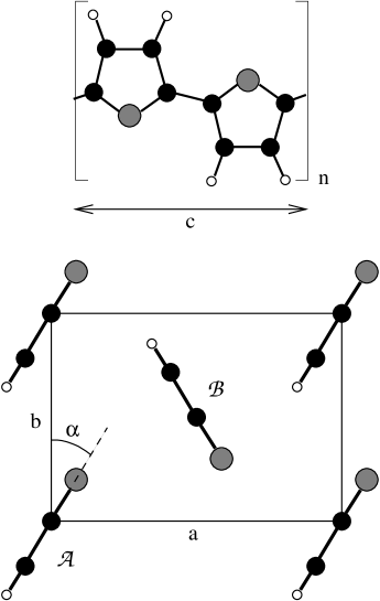
FIG. 1.: Monomer and crystal structure of polythiophene. Top panel: A single chain of polythiophene. Black atoms are carbon, gray sulfur, white hydrogen. Bottom panel: crystal structure (from Ref. [29]) as seen perpendicular to the chain direction ($a$ = 10.5 a.u., $b$ = 14.5 a.u., $c$ = 14.8 a.u., $\alpha=31.2^{\circ}$).

FIG. 2.: The quasi-particle band structure of both an isolated chain of PT (full lines, left) and bulk PT (full lines, right) compared to the DFT-LDA band structure (dashed lines in both pictures).

FIG. 3.: The hole probability along the chain with the electron fixed at 1 a.u. above the inversion center for the two lowest singlet excitons, ¹B_u (above axis) and ¹A_g (below axis), for both the isolated chain (top) and the bulk situation (bottom).

REFERENCES

- [1] J.H. Burroughes, D.D.C. Bradley, A.R. Brown, R.N. Marks, K. Mackay, R.H. Friend, P.L. Bum, A.B. Holmes, Nature 347, 359 (1990).
- [2] J.-L. Brédas, J. Cornil, A.J. Heeger, Adv. Mat. 8, 447 (1996).
- [3] T.W. Hagler, K. Pakbaz, A.J. Heeger, Phys. Rev. B 49, 10968 (1994).
- [4] S.F. Alvarado, P.F. Seidler, D.G. Lidzey, D.D.C. Bradley, Phys. Rev. Lett. 81, 1082 (1998).
- [5] M. Chandross, S. Mazumdar, S. Jeglinski, X. Wei, Z.V. Vardeny, E.W. Kwock, T.M. Miller, Phys. Rev. B 50, 14702 (1994).
- [6] S. Barth, H. Bässler, U. Scherf, K. Müllen, Chem. Phys. Lett. 288, 147 (1998).
- [7] M. Wohlgenannt, W. Graupner, G. Leising, Z.V. Vardeny, Phys. Rev. B 60, 5321 (1999).
- [8] P. Vogl, D.K. Campbell, Phys. Rev. B 41, 12797 (1990).
- [9] G. Brocks, P.J. Kelly, R. Car, Synth. Met. 55-57, 4243 (1993).
- [10] P. Gomes da Costa, R.G. Dandrea, E.M. Conwell, Phys. Rev. B 47, 1800 (1993).
- [11] C. Ambrosch-Draxl, J.A. Majewski, P. Vogl, G. Leising, Phys. Rev. B 51, 9668 (1995).
- [12] R.W. Godby, M. Schlüter, L.J. Sham, Phys. Rev. B 37, 10159 (1988).
- [13] L. Hedin, Phys. Rev. 139, A796 (1965); for a recent review see: F. Aryasetiawan and O. Gunnarsson, Rep. Prog. Phys. 61, 237 (1998).
- [14] E.C. Ethridge, J.L. Fry, M. Zaider, Phys. Rev. B 53, 3662 (1996).
- [15] M. Rohlfing and S.G. Louie, Phys. Rev. Lett. 82, 1959 (1999).
- [16] S.F. Alvarado (private communication).
- [17] J.W. van der Horst, P.A. Bobbert, M.A.J. Michels, G. Brocks, P.J. Kelly, Phys. Rev. Lett. 83, 4413 (1999).
- [18] K. Sakurai, H. Tachibana, N. Shiga, C. Terakura, M. Matsumoto and Y. Tokura, Phys. Rev. B 56, 9552 (1997).
- [19] H.J. de Groot, P.A. Bobbert, and W. van Haeringen, Phys. Rev. B 52, 11000 (1995).
- [20] J. van den Brink and G.A. Sawatzky, in Electronic Properties of Novel Materials-Progress in Molecular Nanostructures, edited by H. Kuzmany, M. Mehring, and S. Roth, AIP Conf. Proc. No. 442 (AIP, New York, 1998), p. 152.
- [21] H.J. Schulz, Phys. Rev. Lett. 71, 1864 (1993), and references therein.
- [22] L.X. Benedict, R.B. Bohn, and E.L. Shirley, Phys. Rev. B 57 R9385 (1998), Phys. Rev. Lett. 80, 4514 (1998); L.X. Benedict and E.L. Shirley, Phys. Rev. B 59, 5441 (1999).
- [23] S. Albrecht, L. Reining, R. Del Sole and G. Onida., Phys. Rev. Lett. 80, 4510 (1998).
- [24] M. Rohlfing and S.G. Louie, Phys. Rev. Lett. 81, 2312 (1998).
- [25] L. Sham and T.M. Rice, Phys. Rev. 144, 708 (1966).
- [26] G. Strinati, Phys. Rev. B 29, 5718 (1984).
- [27] G. Brocks, Synth. Met. 102, 914 (1999).
- [28] G. Brocks, unpublished. With DFT the ground state of a given symmetry can be obtained. The triplet ground state corresponds to the lowest triplet exciton.
- [29] S. Brückner and W. Porzio, Makromol. Chem. 189, 961 (1988).
- [30] Z. Mo, K.-B. Lee, Y.B. Moon, M. Kobayashi, A.J. Heeger, F. Wudl, Macromol. 18, 1972 (1985).
- [31] H.N. Rojas, R.W. Godby, and R.J. Needs, Phys. Rev. Lett. 74, 1827 (1995); for a more detailed account see: M. M. Rieger, L. Steinbeck, I.D. White, H.N. Rojas and R.W. Godby, Comp. Phys. Comm. 117, 211 (1999).
- [32] X. Blase, A. Rubio, S.G. Louie, M.L. Cohen, Phys. Rev. B 52, R2225 (1995).
- [33] F. Bechstedt, K. Tenelsen, B. Adolph, R. Del Sole, Phys. Rev. Lett. 78, 1528 (1997).
- [34] L. Landau and E. Lifschitz, Electrodynamics of Continuous Media (Pergamon, Oxford, 1960), p. 61-62.
- [35] M. Kobayashi, N. Colaneri, M. Boysel, F. Wudl and A.J. Heeger, J. Chem. Phys. 82, 5717 (1985).
- [36] E.L. Shirley, Phys. Rev. B 58, 9579 (1999)
- [37] R. Kersting, U. Lemmer, R.F. Mahrt, K. Leo, H. Kurz, H. Bässler, E.O. Göbel, Phys. Rev. Lett. 70, 3820.
- [38] P. Gomes da Costa and E.M. Conwell, Phys. Rev. B 48, R1993 (1993).
- [39] J.D. Jackson, Classical Electrodynamics (2nd edition) (Wiley, New York, 1975), p. 139-141.
- [40] P.H.L. de Jong, M.Sc. Thesis, Technische Universiteit Eindhoven, 1999.