Extended corresponding-states behavior for particles with variable range attractions

Abstract

We propose an extension of the law of corresponding states that can be applied to systems - such as colloidal suspensions - that have widely different ranges of attractive interactions. We argue that, for such systems, the “reduced” second virial coefficient is a convenient parameter to quantify the effective range of attraction. This procedure allows us to give a simple definition of the effective range of attraction of potentials with different functional forms. The advantage of the present approach is that it allows us to estimate the relative location of the liquid-vapor and solid-fluid coexistence curves exclusively on basis of the knowledge of the pair-potential.

Van der Waals’s Law of Corresponding States expresses the fact that there are basic similarities in the thermodynamic properties of all simple gases. Its essential feature is that if we scale the thermodynamic variables that describe an equation of state (temperature, pressure and volume) with respect to their values at the critical point, all simple fluids obey the same reduced equation of state. Pitzer [1] has given a molecular interpretation of the Law of Corresponding States for classical monoatomic systems using statistical mechanical arguments. This proof is restricted to systems for which the total intermolecular potential can be written as a sum over pair potentials in the form:

$$U=\sum_{i,j}\epsilon\text{ }v(r_{i,j}/\sigma)\qquad.$$ (1)

The essential assumptions are pairwise additivity and the fact that the pair potential can be written as an energy parameter $\epsilon$ times a function of the reduced distance $r/\sigma$. The Law of Corresponding States follows when we assume that the pair potentials of all substances to which the law applies are conformal. Interaction potentials are said to be conformal if their plots can be made to superimpose by adjusting the values of $\epsilon$ and $\sigma$. With these assumptions, the partition function is of the form:

$$Q(N,V,T)=\left[\frac{\sigma^{3}}{\Lambda^{3}}g\left(T^{*},\rho^{*}\right)\right]\qquad,$$ (2)

where $g$ is the same function for all molecules and depends only on $T^{*}=k_{B}T/\epsilon$, the reduced temperature, and $\rho^{*}=N/V\sigma^{3}$ the reduced density[2]. It then follows that many other thermodynamic properties - in particular the pressure - are functions of $T^{*}$ and $\rho^{*}$ only.

Unfortunately the interactions between real molecules are never truly pairwise additive, nor are the pair potentials of different molecules conformal. Even for inert gases the conformality of pair-potentials is only fair. Moreover, the importance of three-body forces restricts the validity of the assumption of pairwise additivity. While only a small family of substances can be described by the original form of the Law of Corresponding States, many fluids conform quite accurately to extended equations-of-state that involve a third parameter. Thus, the compressibility factor $z$ can be expressed as

$$z=\beta P/\rho=f\left(T^{*},\rho^{*},x\right)\qquad,$$ (3)

where $x$ is a third parameter that is usually related to some characteristic feature of the phase diagram of a substance. At first[3] the critical compression factor $z_{c}$ was used for $x$, but $z_{c}$ is hard to determine with high accuracy, and a better choice was sought. The slope of the vapor pressure curve (at a reduced temperature of $T_{r}=0.7$), $\omega$, turned out to be a more convenient choice for $x$ [4, 5]. Various equations of the form $z(T^{*},\rho^{*},\omega)$ have been presented[6], which agree well with the thermodynamic properties for several classes of molecular fluids.

In this Communication we focus on the effect of changing the range of attractive forces in suspensions of spherical colloids. As the range of attraction varies independently of the hard-core radius $\sigma$, the effective interactions are clearly not conformal. It is known that the phase behavior of colloidal suspensions depends strongly on the range of the attractive interactions. However, at present, there is –to our knowledge– no extended law of corresponding states that allows us to make predictions about the phase behavior on the basis of the effective pair potential alone. In fact, a wide variety of non-conformal pair potentials have been used to describe the interactions between colloids with short ranged attraction. It is our aim to formulate an extended law of corresponding states that allows us to compare such different pair potentials. In particular, we have considered the square-well model[7], attractive Yukawa potentials [8, 9], 2n-n Lennard-Jones type potentials[10], the $\alpha$-Lennard-Jones potential used in the description of protein-protein interactions[11, 12], an effective potential reproducing the depletion attractive forces in colloid-polymer mixtures[13], and more complex potentials, which include a repulsive barrier, i.e. the effective two-body potential for mixtures of nonadditive asymmetric hard spheres [14]. At this stage we limit our analysis to the phase behavior around the critical point, but our findings should be generalized to densities away from the critical region, in the spirit of the extended law of corresponding states.

We proceed to calculate the scaling parameters ($\epsilon,\sigma$ and $x$), which stem from the knowledge of the inter-particle potential alone, without any need for further experimental measurement. An obvious choice for the length scale $\sigma$ is the effective hard core diameter. Some care has to be taken in the calculation of $\sigma^{EFF}$ for continuous potentials (such as the Lennard-Jones 2n-n). According to the Weeks-Chandler-Andersen (WCA) method, we separate the potential into attractive $v_{att}$ and repulsive $v_{rep}$ parts[15], and calculate the “equivalent” hard-core diameter for the repulsive part of the potential using the expression suggested by Barker[16]:

$$\sigma^{EFF}=\int_{0}^{\infty}dr\left[1-e^{-v_{rep}(r)/k_{B}T}\right]\qquad.$$ (4)

Two parameters are needed to properly describe the role of attractions: an energy scale and a second quantity related to the range of attraction. At low temperatures, the potential energy per particle in the crystalline phase is given by the value of the pair-potential at the nearest-neighbor separation, multiplied by the number of neighbors (and divided by two, to correct for double counting). This is independent of the functional form of the potential. This makes $v(r_{min})$, the depth of the potential well, our natural choice for the energy scale $\epsilon$. The third parameter that we use is the reduced second virial coefficient, i.e. the second virial coefficient $B_{2}$ divided by the second virial coefficient of hard spheres with a diameter $\sigma^{EFF}$. The second virial coefficient $B_{2}$ can be easily calculated once the functional form of the potential has been specified:

$$B_{2}=2\pi\int_{0}^{\infty}dr\quad r^{2}\left[1-e^{-v(r)/k_{B}T}\right]\qquad,$$ (5)

and the reduced second virial coefficient $B_{2}^{\ast}$ is defined as

$$B_{2}^{\ast}\equiv\frac{B_{2}}{2\pi(\sigma^{EFF})^{3}/3}\qquad.$$ (6)

Note that all three parameters ($\sigma^{EFF},\epsilon$ and $B_{2}^{\ast}$) can be computed only based on the intermolecular potential $v(r)$. In this sense, our approach differs from those extended corresponding states laws that use experimental data to define appropriate scaling parameters. This is particularly useful for the description of colloidal systems where the topology of the phase diagram changes as the range of the attraction is decreased. For instance, it would not be feasible to use the properties at the critical point as scaling parameters, as the critical point may be experimentally inaccessible for sufficiently short-ranged attractions. Our working hypothesis is that for a wide range of colloidal materials, the compressibility factor $z$ is a function of only three parameters, viz.  the reduced temperature $T^{\ast}=k_{B}T/\epsilon$, the reduced density $\rho^{\ast}=N/V(\sigma^{EFF})^{3}$ and the reduced second-virial coefficient $B_{2}^{\ast}$

$$z=f\left(T^{\ast},\rho^{\ast},B_{2}^{\ast}\right)\qquad.$$ (7)

In the literature onhard particles with short-ranged attraction, it is conventional to express the reduced second-virial coefficient in terms of a parameter $\tau$ that is defined through the the following equation [17]:

$$B_{2}^{\ast}\equiv 1-\frac{1}{4\tau}\qquad.$$ (8)

$\tau$ is a measure for the temperature - low (high) $T$ corresponds to low (high) $\tau$. However, $\tau$ is not a linear function of $T$.

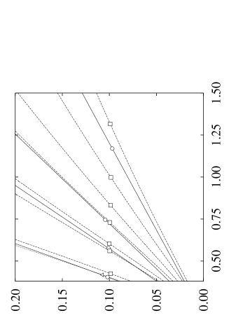
$\tau$ $T^{*}$

FIG. 1.: Stickyness parameter $\tau$ plotted versus the reduced temperature $T^{*}=k_{B}T/\epsilon$ for different potentials. Circles: attractive Yukawa, attractive Yukawa, Squares: Lennard Jones 2n-2, Triangles: $\alpha$-Lennard Jones

In Figure (1) we have plotted the stickyness parameter $\tau$ as a function of the reduced temperature for some of the cases listed in Table I. In the temperature range studied, the stickyness parameter increases almost linearly with the reduced temperature[18]. The figure shows another important feature: if the $\tau-T^{*}$ curves for two different potentials are close at any particular temperature, they tend to be close for all temperatures studied. Such behavior is an indication that the present scheme to compare non-conformal potentials is reasonable. As can be seen from the figure (and from Table I), the value of $\tau$ – and therefore that of the reduced second virial coefficient – at the critical point is remarkably constant (around $\tau\approx 0.1$). This fact had been noted earlier by Vliegenthart and Lekkerkerker[19]. In fact, $\tau$ hardly varies between the limit of extremely narrow attractive wells (Baxter’s adhesive hard-sphere model [17]) and the (van der Waals) limit of infinitely long-ranged attractive wells. Also in models that are a mixture of the Baxter and van der Waals model the value of $\tau$ at the critical point varies only slightly[20].

We mentioned above that the reduced second virial coefficient is a measure for the range of the attractive part of the potential. To make this statement more precise, we have to specify what we mean by the “range” of a potential. Here, we take the following route: there is one system for which the range of the attractive potential is defined unambiguously, namely hard spheres with a square-well attraction

$$u(r)=\left\{{\ \matrix{\ \infty\hfill\cr-\epsilon\hfill\cr 0\hfill\cr}}\right.\quad\matrix{\ {r\leq\sigma}\hfill\cr{\sigma<r\leq\lambda\sigma}\hfill\cr{\lambda\sigma<r}\hfill\cr}\qquad.$$ (9)

A logical choice for a dimensionless measure for the range of the attractive part of the potential is $R\equiv\lambda-1$. In the spirit of our extended corresponding states approach, we now define  the range of an arbitrary attractive potential to be equal to the range of that square-well potential that yields the same reduced second virial coefficient at the same reduced temperature. The reduced second virial coefficient of a square-well potential is given by

$$B_{2}^{*}=1+\left[\lambda^{3}-1\right]\left(1-e^{1/T^{*}}\right)\qquad,$$ (10)

and hence

$$\tau=\frac{1}{4\left[\lambda^{3}-1\right]\left(e^{1/T^{*}}-1\right)}\qquad.$$ (11)

Using this mapping onto the square-well system, we have computed the effective range of the attractive part of the potential for a number of different potential functions that have been used to describe colloidal suspensions or globular protein solutions. In general, the range of attraction is still temperature dependent. In Table I, we have collected the values of $R$ at the temperature corresponding to the liquid-vapor critical point. In the same table, we also give the value for the “stickyness” parameter $\tau$ at the critical temperature.

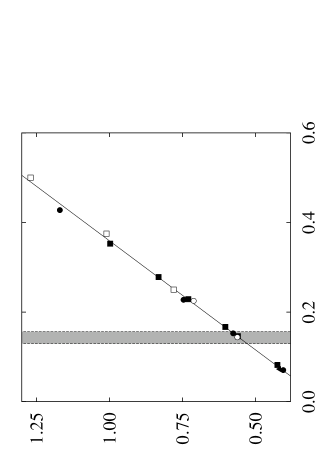
$T^{*}_{c}$ $R$

FIG. 2.: The reduced temperature at the liquid-gas critical point $T^{*}_{c}=k_{B}T_{c}/\epsilon$ plotted versus the range of attractions $R=\lambda-1$ of the equivalent square well system. As the range becomes shorter than the threshold value $\approx 0.14$, the liquid-gas transition becomes metastable. Filled Circles: attractive Yukawa, Filled Squares: Lennard Jones 2n-n, Filled Triangles: $\alpha$-Lennard Jones, Open Squares: Square Well, Open Circles: effective Colloid-Colloid interaction

In Figure (2), we show the relation between $T_{c}^{*}$, the reduced critical temperature and $R$, the range of the attractive potential. In the temperature range studied, the relation between $R$ and $T_{c}^{*}$ is surprisingly linear – although, again, we know that this linear relation cannot hold for values of $R$ very close to zero – and obeys the simple relation:

$$T_{c}^{*}\approx 0.26+2.1R\qquad.$$ (12)

The range of the attractive part of the potential determines whether a given system can exhibit a stable liquid-vapor transition or whether this transition is preempted by freezing. The disappearance of the liquid-vapor transition in systems with short-ranged attraction was first noted in theoretical work by Gast, Russel and Hall[21]. This work has subsequently been placed on a firmer theoretical footing by Lekkerkerker et al[22]. Evidence for the disappearing of the liquid-vapor critical point comes from both simulation[11, 9] and experiment[23]. All authors agree that the liquid-vapor transition disappears for sufficiently short-ranged attraction. However, estimates differ for the value of $R$ where this change in the phase diagram takes place. Estimates for $R$ vary from $0.1$ to almost $0.4$. Part of the reason why the different estimates for the critical value of $R$ appear inconsistent is that the various authors have studied systems with non-conformal interaction potentials and, more importantly, have used different definitions for the range. The advantage of the present approach is that we have a unique way to define the range of the attractive potential for widely different interaction potentials. When we consider the available data for the 2n-n Lennard-Jones potentials, the $\alpha$-Lennard-Jones potential, and the attractive Yukawa system, we find that in every case the boundary between stable and meta-stable liquid-vapor transitions is located within a narrow band between $R=0.13$ and $R=0.15$. In Figure (2) critical points plotted to the right of the vertical $R\approx 0.14$ band refer to a stable transition, while points to the left are metastable. To date no simulation has computed the threshold value for square-well particles. A rough estimate of $R\approx 0.25$ has been calculated using a simple van der Waals model for both the fluid and the solid phase[24] and from a simple cell model with some phenomenological character[25]. For $R=0.85$, theoretical estimates suggest that in this case the critical point is stable[26].

The predictive power of our approach based on pair potentials is expected to break down when three-body interactions become important. We have also tested our theory for more complex pair potentials, which included a repulsive barrier[14]. Here too we have found deviations from extended corresponding states behavior: in several cases the calulated $\tau$ parameter, at the critical point, lies much below the constant value of $0.10$, and the mapping onto the equivalent square-well system yields unphysically small attraction ranges $R$. The repulsive barrier alters the effective size of the particle, especially at low temperatures, but our WCA decomposition of the effective potential limits the repulsive contribution to the hard body term.

In summary, we have formulated a simple extended corresponding states principle that allows us to make predictions about the topology of the phase diagram of suspensions of spherical colloids with variable range attraction. The scaling parameter $\sigma$, $\epsilon$ and $B_{2}^{*}$ can all be derived directly from knowledge of the pair-potential. Moreover, this procedure allows us to give an unambiguous definition for the range of the attractive part of the potential. By analysing a number of simulation data for different model systems, we find that the liquid-vapor transition becomes metastable with respect to the freezing transition when the range of the attraction becomes less than approximately $0.14$.

$\star\star\star$
The work of the FOM Institute is part of the research program of “Stichting Fundamenteel Onderzoek der Materie” (FOM) and is supported by NWO. We gratefully acknowledge discussions with Fernando Fernandez. We also thank N.Kern and H.N.W.Lekkerkerker for critical reading of the manuscript and for useful suggestions. MGN acknowledges financial support from EU contract ERBFMBICT982949.

	$T^{*}_{c}$	$\tau$	R
Square Well[7]
	2.61	0.0765	1.000
	1.79	0.0766	0.750
	1.27	0.0942	0.500
	1.01	0.0924	0.375
	0.78	0.1007	0.250
Yukawa[8, 9]
	1.170	0.0969	0.427
	0.715	0.1044	0.227
	0.576	0.1009	0.153
	0.412	0.1020	0.070
2n-n[10]
	1.316	0.0990	0.476
	0.997	0.0983	0.353
	0.831	0.0987	0.278
	0.730	0.0996	0.229
	0.603	0.1001	0.167
	0.560	0.0997	0.146
	0.425	0.0986	0.082
$\alpha$-LJ[11]
	0.418	0.1073	0.073
Colloid[13]
	0.712	0.0970	0.225
	0.562	0.1023	0.144
Asymm. hard-spheres[14]
	0.186	0.0744	0.005
	0.173	0.0758	0.003
	0.164	0.0788	0.002

TABLE I.: Values of $T^{*}$, $\tau$ and the range of the equivalent square well system $R$ for different potentials, and for different ranges, calculated at the liquid-gas critical point

REFERENCES

- [1] K.E.Pitzer, J.Chem.Phys. 7, 583 (1939)
- [2] D.A.McQuarry Statistical Mechanics (Harper Collins Publishers, New York, 1976)
- [3] O.A.Hougen, K.M.Watson, Chemical Processes Principles (Wiley, New York, 1947)
- [4] L.Riedel, Chem.Ing.Tech. 26, 83 (1954)
- [5] K.S.Pitzer, D.Z.Lippman, R.F.Curl, C.M.Huggins and D.E.Petersen, J.Am.Chem.Soc. 77, 3433 (1955)
- [6] Twelve equations of this type are described in D.R.Schreiber, K.S.Pitzer, Fluid Phase Equil. 46, 113 (1989)
- [7] We considered the results from J.R.Elliot and L.Hu, J.Chem.Phys 110 (6) 3043 (1999); other estimates of the fluid-fluid critical point are given in L.Vega, E.deMiguel, L.F.Rull, G.Jackson, and I.A.McLure, J.Chem.Phys. 96, 2296 (1996) and in J.Chang and S.I.Sandler, Mol.Phys. 81, 745 (1994).
- [8] E.Lomba and N.G.Almarza, J.Chem.Phys. 100, 8367 (1994)
- [9] M.Hagen and D.Frenkel, J.Chem.Phys. 101, 4093 (1994)
- [10] G.A.Vliegenthart, J.M.F.Lodge, and H.N.W.Lekkerkerker, Physica A 263, 378 (1999)
- [11] E.J.Meijer and F.ElAzhar, J.Chem.Phys. 106 4678 (1997)
- [12] P.R.tenWolde and D.Frenkel, Science 277 1975 (1997)
- [13] E.J.Meijer and D.Frenkel, J.Chem.Phys. 100(9) 6873 (1994)
- [14] M.Dijkstra, Phys.Rev.E 58 (6) 7523 (1998); M.Dijkstra, R.van Roij and R.Evans, Phys.Rev.E 59 (5) 5744 (1999)
- [15] H.C.Andersen, J.D.Weeks and D.Chandler, Phys. Rev. A 4 1579 (1971)
- [16] J.A.Barker and D.Henderson, Rev. Mod. Phys. 48 587 (1976)
- [17] R.J.Baxter, J.Chem.Phys. 49 2270 (1968)
- [18] However, as can be seen from Eqn. (11), the linear relation should break down for sufficiently low reduced temperatures.
- [19] G.A.Vliegenthart and H.N.W.Lekkerkerker, J.Chem.Phys. 112 (12) 5364 (2000)
- [20] M.G.Noro, N.Kern and D.Frenkel, Europhys. Lett. 48 (3) 332 (1999)
- [21] A.P.Gast, C.K.Elliot and W.B.Russel, J.Coll.Int.Sci. 96 (1) 251 (1983)
- [22] H.N.W.Lekkerkerker, W.C.K.Poon, P.N.Pusey, A.Stroobants and P.B.Warren, Europhys.Lett. 20 (6) 559 (1992)
- [23] S.M.Illet, A.Orrock, W.C.K.Poon and P.N.Pusey, Phys.Rev.E 51 (2) 1344 (1995)
- [24] A.Daanoun, C.F.Tejero and M.Baus, Phys.Rev.E 50 (4) 2913 (1994)
- [25] N.Asherie, A.Lomakin and G.Benedek, Phys.Rev.Lett. 77 (23) 4832 (1996)
- [26] W.W.Lincoln, J.J.Kozac and K.D.Luks J.Chem.Phys. 62 (2) 2171 (1975); K.U.Co, K.D.Luks and J.J.Kozac, Mol.Phys. 36 (6) 1883 (1978)