Nucleation on top of islands in epitaxial growth

Abstract

We develop a theory for nucleation on top of islands in epitaxial growth based on the derivation of lifetimes and rates governing individual microscopic processes. These in particular include the encounter rate of $j$ atoms in a state, where in total $n\!\geq\!j$ atoms are present on top of the island, and the lifetime of this state. The latter depends strongly on the additional step edge barrier $\Delta E_{\rm S}$ for descending atoms. We present two analytical approaches complemented by kinetic Monte Carlo simulations. In the first approach we employ a simplified stochastic description, which allows us to derive the nucleation rate on top of islands explicitly, if the dissociation times of unstable clusters can be neglected. We find that for small critical nuclei of size $i\!\leq\!2$ the nucleation is governed by fluctuations, during which by chance $i\!+\!1$ atoms are present on the island. For large critical nuclei $i\!\geq\!3$ by contrast, the nucleation process can be described in a mean-field type manner, which for large $\Delta E_{\rm S}$ corresponds to the approach developed by Tersoff et al. [Phys. Rev. Lett. 72, 266 (1994)]. In both the fluctuation-dominated and the mean-field case, various scaling regimes are identified, where the typical island size at the onset of nucleation shows a power law in dependence on the adatom diffusion rates, the incoming atom flux, and the step edge crossing probability $\exp(-\Delta E_{\rm S}/k_{\rm B}T)$. Although it is possible to extend the simplified approach to more general situations, its applicability is limited, if dissociation rates of metastable clusters enter the problem as additional parameters. For such situations the second semi-analytical approach becomes superior. This approach is based on novel rate equations , which can easily be solved numerically. Both theoretical approaches yield good agreement with Monte Carlo data. Implications for various applications are pointed out.

I Introduction

A fundamental problem in the theory of thin film growth [1] is the question, under which condition flat, two-dimensional films form on the substrate surface in contrast to mutually-separated, three-dimensional clusters. For films growing under equilibrium conditions, this question has been answered many years ago: If the interfacial tension between the substrate and adsorbate is larger than the difference of the respective surface free energies, then cluster formation is preferred (“Volmer-Weber growth” [2]), while a smaller (or equal) interfacial tension leads to the formation of flat films (“Van-der Merwe growth”). An intermediate case is the “Stranski-Krastanov growth” mode,[3] where cluster formation sets in after the thickness of an initially smooth film exceeds a critical height. This case may be understood from an interfacial tension that varies with the film thickness. More recently, the influence of strain effects on equilibrium film morphologies has been investigated by various authors.[4]

Films developing in the process of molecular beam epitaxy (MBE) are usually not in thermodynamic equilibrium.[5]. Rapid growth of films is achieved by a high supersaturation of the vapor, and growth kinetics is governed by evaporation, diffusion and aggregation processes far from equilibrium. Determining the film morphology in this situation is a problem of stochastic dynamics. (For a recent review on both kinetically and thermodynamically induced instabilities in MBE see ref. [6].) During the MBE experiment, two-dimensional islands composed of adsorbate atoms form on the substrate. If these islands coalesce before stable clusters nucleate on top of the islands in the second layer, a flat two-dimensional film results. By contrast, if the onset of second layer nucleation precedes island coalescence, then three-dimensional cluster formation is obtained. The term “second layer nucleation” should not be taken literally here but rather should apply to the formation of stable nuclei composed of $(i\!+\!1)$ atoms on top of islands in general. As for the equilibrium structures, it might be possible that cluster formation sets in above a certain film thickness, when the relevant parameters governing the nucleation of stable clusters on top of islands (see below) depend sensitively on the film thickness. However, despite this similarity of the possible growth processes with the equilibrium growth modes, it should be noted that the dynamic problem is very different. In MBE flat films can be produced even if the adsorbate does not wet the substrate.[5]

The first theory for second layer nucleation in MBE was set up by J. Tersoff, A. W. Denier van der Gon, and R. M. Tromp,[7] which will be referred to as “TDT approach” in the following. Solving the stationary diffusion equation in the presence of an incoming flux and employing classical nucleation theory,[1] these authors succeeded in deriving an explicit expression for the rate of nucleation $\Omega(R)$ on top of circular shaped islands of radius $R$. Assuming all island radii to evolve approximately as the mean island radius $R(t)\sim t^{1/2}$ at time $t$ (this situation will be referred to as the “single-island model” in the following), they calculated the fraction $f_{0}(t)$ of “covered islands” (i.e. on top of which a stable cluster has nucleated) from $\Omega(R)$. It turned out that $f_{0}(t)$ rises from zero to one in the vicinity of a “critical time” $t_{c}$, which allows one to define a critical island radius $R_{c}\!\equiv\!R(t_{c})$ for second layer nucleation. A simple criterion for the occurrence of “rough multilayer” as opposed to smooth “layer-by-layer growth” is that $R_{c}$ is smaller than the mean distance $l$ between islands in the first layer.

An important factor controlling the film morphology is the additional step edge barrier $\Delta E_{\rm S}\!=\!E_{\rm S}\!-\!E_{0}$ (Ehrlich-Schwoebel barrier[8]) that has to be surmounted by an adatom in addition to the bare surface diffusion barrier $E_{0}$, when an adatom crosses an island edge.[9] For larger $\Delta E_{\rm S}$ one expects adatoms to remain longer on islands and therefore to accumulate more easily, which would lead to an increased second layer nucleation rate $\Omega(R)$ and a smaller $R_{c}$. In fact, the theory predicts that only for sufficiently large $\Delta E_{\rm S}$ three-dimensional clusters can occur on the substrate (for an alternative possibility see however ref. [10]). Using the TDT approach, $\Delta E_{\rm S}$ was estimated for a variety of different systems. [11, 12, 13, 14, 15]

An alternative approach for treating the problem of second layer nucleation within a stochastic description based on scaling arguments was developed recently by us.[16] It was shown that for $i\!=\!1$ the TDT approach is not applicable, but the detailed treatment of fluctuations with only two atoms on top of the island yields a correct description of the process (see also ref.[17]; for an earlier approach focusing on one dimension see ref. [18]). In this work we will extend our former study of second layer nucleation by means of both kinetic Monte Carlo simulations and scaling analysis. In particular, we will show that the mean-field assumptions underlying the TDT approach are valid for large critical nuclei $i\!\geq\!3$, while for small critical nuclei $i\!=\!1,2$ second layer nucleation is dominated by fluctuations. Furthermore, we develop a novel rate equation approach, which allows one to calculate the time-development of cluster configurations on compact two-dimensional islands under quite general conditions.

From the outset, one should distinguish between nucleation on top of islands with compact shape as opposed to nucleation on islands with strongly ramified shape. In the latter situation, diffusion of adatoms on the islands becomes a rather complex phenomenon due to the confined motion along branches of various lengths.[19] We restrict our discussion to nucleation on compact islands here. Intuitively, one would expect second layer nucleation on ramified islands to be unlikely, so that this restriction is of minor importance. Moreover, it should be noted that even for compact shapes, the island boundaries may have a fractal or, more precisely, self-affine [20] structure (this is the case e.g. for Eden clusters [21]). Then the microscopic step edge barrier [22] can vary strongly along the island boundary. In any case we will always understand $\Delta E_{\rm S}$ as an effective barrier (see below and ref. [23]).

Parameters governing the second layer nucleation are the incoming atom flux $F$, the jump rate $D/a^{2}$ of adatoms, the step edge barrier $\Delta E_{\rm S}$, and various dissociation rates of unstable clusters of size $s\!\leq\!i$. If the bond energies of the unstable clusters (i.e. of clusters of size $s\!\leq\!i$) are negligibly small, then the nucleation rate $\Omega(R)$ and critical radius $R_{c}$ depend only on two dimensionless parameters. These are the ratio

$$\Gamma\equiv\frac{D}{Fa^{4}}$$ (1)

(with $a$ being the lattice spacing in the substrate plane) and the edge crossing probability

$$\alpha\equiv\exp\left(-\frac{\Delta E_{\rm S}}{k_{\rm B}T}\right)\,.$$ (2)

Based on a simplified stochastic description (see also ref. [16]) we will argue that for small critical nuclei $i\!=\!1,2$ the mean number of atoms on top of the island is smaller than one and the stable nucleus is formed due to fluctuations. This gives rise to four scaling regimes in an $\alpha-\Gamma$ diagram, where $R_{c}\sim\Gamma^{\gamma}\alpha^{\mu}$ with different exponents $\gamma$ and $\mu$. For $i\!\geq\!3$ by contrast, nucleation starts out from a situation with many atoms present on the island. Under these circumstances, three different scaling regimes can be identified, and two of them correspond to the ones predicted by the TDT approach. By comparing $R_{c}$ with the mean distance $l$ between islands on the substrate surface, the transition line separating rough multilayer from smooth layer-by-layer growth is identified in the $\alpha-\Gamma$ diagram. When the bond energies of unstable clusters become appreciable, the corresponding dissociation rates enter the problem as additional relevant parameters. It becomes difficult then to separate scaling regimes in practice, and the simplified stochastic description becomes of limited value. However, by employing the novel rate equation approach it is still possible to determine $f_{0}(t)$ and $R_{c}$ in a simple manner.

Moreover, we will discuss how to derive the fraction of $f(t)$ of covered islands, when one relaxes the assumption that all island radii evolve as the mean radius $R(t)$. In the time regime of almost constant island density (“saturation regime” preceeding island coalescence[24]) we can define an effective “capture area” for adatoms by the Voronoi cell for each island.[25] In order to calculate $f(t)$ for the “multi-island model” from $f_{0}(t)$, one needs to know the probability distribution of islands with a certain size and capture area, when the saturation regime is reached.

The paper is organized as follows. In Sec. II we give a short review on basic concepts used in the description of submonolayer growth and discuss in part II A important quantities and equations underlying the physical processes involved. In part II B we summarise the results of the TDT approach. We then continue with a detailed description of the simulation techniques in Sec. III and test the equivalence of the multi-island and single-island model.

In Sec. IV a simplified stochastic description of second layer nucleation is first presented in its general methodology and subsequently employed to small and large critical nuclei. It is instructive to observe the different physical conditions that lead to the nucleation event in the two cases. After showing that the treatment of metastable clusters is rather complicated within the simplified description, we discuss in Sec. V a general approach for second layer nucleation on the basis of novel rate equations. Sec. VI concludes the paper with a summary and discussion of the most important results as well as an outlook to further research.

II Basic quantities and concepts

A Atomistic processes in thin film growth

In MBE atoms are deposited on a substrate surface with a rate $Fa^{2}$ per unit cell. At very high temperatures the adatoms reevaporate but under ordinary conditions this reevaporation can be neglected or effectively taken into account by a reduced deposition rate. Once an adatom is deposited, it starts a thermally activated diffusive motion with jump rate $D/a^{2}\propto\exp(-E_{0}/k_{\rm B}T)$. Adatoms come into contact as time progresses, and form islands that are held together by some bonding energy. While unstable islands of small size $s\leq i$ dissociate, islands with size $s>i$ are stable (on all relevant time scales of the experiment). An island of size $s=i$ is called a critical nucleus.[26]

Islands of larger size are formed by aggregation of adatoms (or small mobile islands) to existing immobile islands, and by coalescence. These processes lead to an island size distribution which becomes broader with increasing time. In the submonolayer regime, the most important physical questions are: (i) How large is the density $\rho_{x}(t)$ of stable islands on the substrate surface at time $t$? (ii) What is the form of the distribution $\chi_{s}(s,t)$ of island sizes $s$ at time $t$ (with $s$ being the number of atoms forming the island)? (iii) What do the stable islands look like? These questions have been extensively studied in the past, both by experiment and by theory. We will briefly summarise those results, which are relevant for the following analysis.

The typical behavior of $\rho_{x}(t)$ is depicted in Fig. 1. Also shown is the adatom density $\rho_{1}(t)$. As suggested by Amar and Family, [24] one may distinguish between four different time regimes: The low-coverage regime $L$ where $\rho_{x}(t)$ increases with $t$ and $\rho_{x}(t)\!<\!\rho_{1}(t)$, the intermediate coverage regime I, where $\rho_{x}(t)$ increases with $t$ and $\rho_{x}(t)\!>\!\rho_{1}(t)$, the saturation regime S (called aggregation

FIG. 1.: The densities $\rho_{1}(t)$ and $\rho_{x}(t)$ of adatoms and stable islands as obtained in a kinetic Monte Carlo simulation modeling submonolayer growth (for an analogous figure see e.g. ref. [24]). The different time regimes of low coverage L, intermediate coverage I, saturation S and coalescence C are indicated.

regime A in ref. [24]), where $\rho_{x}(t)$ stays approximately constant, and the coalescence regime C, where $\rho_{x}(t)$ strongly decreases due to coalescence of stable clusters. At high coverages $\theta\equiv Fa^{2}t$, the monomer density $\rho_{1}(t)$ becomes small (see Fig. 1), and the standard rate equations for submonolayer growth [1] predict $\rho_{x}$ to evolve as

$$\rho_{x}(t) \propto \left(\frac{D}{Fa^{4}}\right)^{-\frac{\scriptstyle i}{\scriptstyle i+2}}(Fa^{2}t)^{\frac{\scriptstyle 1}{\scriptstyle i+2}}\,e^{E_{i}/(i+2)k_{\rm B}T}$$ (4)

$$=\Gamma^{-\frac{\scriptstyle i}{\scriptstyle i+2}}\,\theta^{\frac{\scriptstyle 1}{\scriptstyle i+2}}\,e^{E_{i}/(i+2)k_{\rm B}T}\,,$$

where $E_{i}$ is the bonding energy of the critical nucleus in its preferred atomic configuration.

It should be noted that eq. (4) is not valid in the saturation regime S, where the densities of islands with subcritical and critical size are very small (unless there are metastable subcritical nuclei). In this regime almost all adatoms being deposited attach to preexisting stable islands, so that $\rho_{x}(t)$ stays constant, $\rho_{x}(t)=\rho_{x}$. Within the standard rate equation approach, this effect may be accounted for by a proper dependence of the “capture numbers” on the adatom density $\rho_{1}(t)$ (for a detailed discussion of this point in relation to experiments see ref. [27]). The scaling of $\rho_{x}$ with $\Gamma$, however, is still correct in regime S,

$$\rho_{x}\propto\Gamma^{-\frac{\scriptstyle i}{\scriptstyle i+2}}\,.$$ (5)

One of the most detailed studies of the island size distribution has been performed by Amar and Family [24] based on the scaling ansatz [28, 29, 30]

$$\chi_{s}(s,t)=\frac{1}{\langle s(t)\rangle}\,f\Bigl{(}\frac{s}{\langle s(t)\rangle}\Bigr{)}\,.$$ (6)

Here $\chi_{s}(s,t)=\rho_{s}(t)/\rho_{\rm tot}(t)$ is the probability that an island has size $s$; ($\rho_{s}(t)$ is the density of islands with size

FIG. 2.: Typical island morphologies as obtained in kinetic Monte Carlo simulations (a) for strictly irreversible attachment and (b) for irreversible attachment with local relaxation, in the absence of preferred growth directions. For the simulation technique of the local relaxation process see Sec. III and Fig. 3.

$s$ and $\rho_{\rm tot}(t)$ is the total island density). $\langle\ldots\rangle$ denotes an average over $s$ with respect to $\chi_{s}(s,t)$. From (6) follows, for $\langle s^{m}\rangle\!<\!\infty$, $\langle s^{m}\rangle=\langle s\rangle^{m}\int_{0}^{\infty}dx\,x^{m}f(x)$, and taking $m=0,1$ one obtains $\int dxf(x)=\int dx\,xf(x)=1$. The mean island size $\langle s(t)\rangle$ is given by $\langle s(t)\rangle=\sum_{s=1}^{\infty}s\rho_{s}(t)/\rho_{\rm tot}(t)=\theta/\rho_{\rm tot}(t)a^{2}$. In the saturation regime S, in particular, where $\rho_{\rm tot}\simeq\rho_{x}$, since the density of islands with subcritical and critical size is small, it follows from eq. (5)

$$\langle s(t)\rangle\simeq\frac{\theta}{\rho_{x}a^{2}}\propto\theta\,\Gamma^{\frac{\scriptstyle i}{\scriptstyle i+2}}\,.$$ (7)

The relation $\langle s(t)\rangle\simeq theta/\rho_{x}a^{2}=Ft/\rho_{x}$ can also be understood more directly, since the increase of $\langle s(t)\rangle$ with $t$ is given by the flux times the mean capture area $\rho_{x}^{-1}$ of adatoms.

The scaling function $f(u)$ was suggested to have the form [31]

$$f(u)=C_{i}u^{i}\exp(-ia_{i}u^{1/a_{i}})$$ (8)

in regime S. This function has a maximum at $u\!=\!1$ and the two conditions $\int dxf(x)=\int dx\,xf(x)=1$ determine the parameters $C_{i}$ and $a_{i}$. Equations (6-8) have been shown to give a fairly good approximation of some simulations and experiments.

The problem of the island shapes is not yet well understood,[5] but one may roughly answer the third question posed above as follows. For strictly irreversible attachment, where local relaxation of atoms due to fast edge diffusion is suppressed, one obtains dendritic or random fractal structures. Dendritic growth is preferred at low $T$ or small $F$, and a shape transition from dendritic to random fractal structures has been found e.g. for Ag/Pt(111) upon lowering the deposition flux.[32] An example for a random fractal structure obtained in a computer simulation is shown in Fig. 2a. At high temperatures, edge diffusion becomes relevant, and polygonal or “irregular” compact island morphologies develop (see e.g. ref. [33]). An example for an irregular structure is shown in Fig. 2b.

As mentioned in the Introduction, for the study of second layer nucleation we will focus on compact island shapes. Moreover, second layer nucleation in the intermediate regime I is unlikely to occur, since the island radii in this regime are typically smaller than the critical radius $R_{c}$. We therefore consider the second layer nucleation in the saturation regime S, where eqs. (5-8) apply.

B TDT Approach

In the TDT approach, [7] one starts by calculating the adatom density $\rho_{1}^{\scriptscriptstyle\rm st}$ on a circular island with radius $R$ in the stationary state. The stationary diffusion equation with the incoming atom flux acting as a source term reads

$$D\left[\frac{\partial^{2}}{\partial r^{2}}+\frac{1}{r}\frac{\partial}{\partial r}\right]\rho_{1}^{\scriptscriptstyle\rm st}+F=0\,,$$ (9)

and it is supplemented by the boundary conditions ($\alpha=\exp(-\Delta E_{\rm S}/k_{\rm B}T)$)

$$\frac{\partial\rho_{1}^{\scriptscriptstyle\rm st}}{\partial r}\Bigl{|}_{r=0}=0\,,\hskip 8.5359pt-\frac{\partial\rho_{1}^{\scriptscriptstyle\rm st}}{\partial r}\Bigl{|}_{r=R}=\frac{\alpha}{a}\,\rho_{1}^{\scriptscriptstyle\rm st}\Bigl{|}_{r=R}\,,$$ (10)

where $a/\alpha$ is commonly referred to as the “Schwoebel length”.[34] The boundary conditions express the fact that the current density $-D\partial\rho_{1}^{\scriptscriptstyle\rm st}/\partial r$ must vanish at the origin and that at the edge it is given by the density $\rho_{1}$ times the “velocity” (rate times lattice spacing) $(D\alpha/a^{2})a$ to cross the step edge barrier. The solution of eqs. (9,10) is

$$\rho_{1}^{\scriptscriptstyle\rm st}(r)\!=\!\rho_{1}^{\scriptscriptstyle\rm st}(0)\!-\!\frac{Fr^{2}}{4D}\,,\hskip 14.22636pt\rho_{1}^{\scriptscriptstyle\rm st}(0)\!=\!\frac{FR^{2}}{4D}\left(1\!+\!\frac{2a}{\alpha R}\right)\,.$$ (11)

According to standard rate equation theory [1] the local nucleation rate is proportional to $D\rho_{1}^{i\!+\!1}$, so we obtain from eq. (11)

$$\Omega(R) = \kappa\frac{D}{a^{2}}\int_{0}^{R}\,\frac{2\pi rdr}{a^{2}}[\rho_{1}^{\scriptscriptstyle\rm st}(r)a^{2}]^{i\!+\!1}$$ (12)

$$= \frac{4\pi\kappa\Gamma^{-(i\!+\!1)}}{(i\!+\!2)\alpha^{2(i\!+\!2)}}\frac{D}{a^{2}}\left(\frac{\alpha R}{2a}\right)^{i\!+\!2}\left[\left(1\!+\!\frac{\alpha R}{2a}\right)^{i\!+\!2}\!-\!1\right]$$ (13)

$$\simeq \left\{\begin{array}[]{ll}\displaystyle 4\pi\kappa\Gamma^{-(i\!+\!1)}\alpha^{-(i\!+\!1)}\frac{D}{a^{2}}\left(\frac{R}{2a}\right)^{i\!+\!3}\,,&\displaystyle\alpha\ll\frac{2a}{R}\\[14.22636pt] \displaystyle\frac{4\pi\kappa\Gamma^{-(i\!+\!1)}}{i\!+\!2}\frac{D}{a^{2}}\left(\frac{R}{2a}\right)^{2(i\!+\!2)}\,,&\displaystyle\alpha\gg\frac{2a}{R}\end{array}\right.$$ (16)

where $\kappa$ is a constant.

For a given time evolution of the island radius $R\!=\!R(t)$, one can calculate the probability $f_{0}(t)$ for a stable nucleus to have formed on top of the island up to time $t$ as follows: The increase $f_{0}(t+\Delta t)\!-\!f_{0}(t)$ in a small time interval $\Delta t$ is equal to the probability $[1-f_{0}(t)]$ that up to time $t$ no stable nucleus has formed times the probability $\Omega(R(t))\Delta t$ that the nucleation takes place in the time interval $[t,t\!+\!\Delta t]$. Taking the limit $\Delta t\to 0$ and solving the corresponding differential equation with the initial condition $f_{0}(0)\!=\!0$ yields

$$f_{0}(t)=1-\exp\left[-\int_{0}^{t}dt^{\prime}\,\Omega(R(t^{\prime}))\right]\,.$$ (17)

For compact island growth during an MBE experiment, we have $R(t)\!\sim\!\langle s(t)\rangle^{1/2}$ and thus from eq. (7)

$$\frac{R(t)}{a}=A(Fa^{2}t)^{1/2}\Gamma^{i/2(i\!+\!2)}$$ (18)

with $A$ being some constant. Inserting this growth law into (16,17) yields

$$f_{0}(t) = 1-\exp\left[-\frac{2\Gamma^{\scriptstyle-\frac{i}{i\!+\!2}}}{A^{2}Fa^{4}}\int_{0}^{R(t)}dr\,r\Omega(r)\right]$$ (22)

$$\simeq\left\{\begin{array}[]{ll}\displaystyle 1-\exp\left[-C_{\scriptscriptstyle<}\Gamma^{\scriptstyle-\frac{i(i\!+\!3)}{i\!+\!2}}\alpha^{-(i\!+\!1)}\Bigl{(}\frac{R}{a}\Bigr{)}^{i\!+\!5}\right]\,,&\displaystyle\alpha\ll\frac{2a}{R(t)}\\[17.07182pt] \displaystyle 1-\exp\left[-C_{\scriptscriptstyle>}\Gamma^{\scriptstyle-\frac{i(i\!+\!3)}{i\!+\!2}}\Bigl{(}\frac{R}{a}\Bigr{)}^{2(i\!+\!3)}\right]\,,&\displaystyle\alpha\gg\frac{2a}{R(t)}\end{array}\right.$$

where $C_{\scriptscriptstyle>}\!\equiv\!(2^{-2(i\!+\!1)}\pi\kappa A^{-2})/[(i+2)(i+3)]$ and $C_{\scriptscriptstyle<}\!\equiv\!2^{-i}\pi\kappa A^{-2}$. In going from the first to the second line in (22) we have used that the integral over $r$ is dominated by the upper integration bound $R(t)$ (for $R(t)/a\gg 1$). It follows that the critical radius scales as

$$R_{c}\sim\Gamma^{\gamma}\alpha^{\mu}\,,$$ (23)

where

$$\gamma=\left\{\begin{array}[]{l@{\hspace{0.3cm}}l}\displaystyle\frac{i(i\!+\!3)}{(i\!+\!2)(i\!+\!5)}\,,\hfil\hskip 8.5359pt&\displaystyle\alpha\ll\Gamma^{i/[2(i\!+\!2)]}\\[11.38092pt] \displaystyle\frac{i}{2(i\!+\!2)}\,,\hfil\hskip 8.5359pt&\displaystyle\alpha\gg\Gamma^{i/[2(i\!+\!2)]}\end{array}\right.$$ (24)

and

$$\mu=\left\{\begin{array}[]{l@{\hspace{0.3cm}}l}\displaystyle\frac{(i\!+\!1)}{(i\!+\!5)}\,,\hfil\hskip 8.5359pt&\displaystyle\alpha\ll\Gamma^{i/[2(i\!+\!2)]}\\[11.38092pt] \displaystyle 0\,,\hfil\hskip 8.5359pt&\displaystyle\alpha\gg\Gamma^{i/[2(i\!+\!2)]}\end{array}\right.$$ (25)

Equations (23-25) predict that for large step edge barriers, $R_{c}$ depends strongly on $\Delta E_{\rm S}$, $R_{c}\sim\exp[-(i+1)\Delta E_{\rm S}/(i+5)k_{\rm B}T]$, while for small barriers, $R_{c}$ becomes independent of $\Delta E_{\rm S}$. For $i=1$ in particular, one finds $R_{c}\sim\Gamma^{2/9}\alpha^{1/3}$ for $\alpha\ll\Gamma^{1/6}$ and $R_{c}\sim\Gamma^{1/6}$ for $\alpha\gg\Gamma^{1/6}$.

III Kinetic Monte Carlo Simulations

Kinetic Monte Carlo simulations are a well-established technique for modeling MBE experiments.[35, 36, 37, 38] In our investigation of second layer nucleation, we adopt a simulation scheme similar to previous, successful models of surface growth kinetics.[37, 30] We chose a substrate with fcc(111) symmetry, since surfaces of that kind are often studied in metal epitaxy, and commonly exhibit high $\Delta E_{\rm S}$. In a full simulation scheme of the growth kinetics (multi-island model), we include all processes of evaporation, diffusion and aggregation occurring in the MBE experiment. By analyzing the set of islands of various size on the substrate, we determine the fraction $f(t)$ of covered islands at time $t$. On the other hand, we consider, as in the TDT approach, only one island with the mean radius $R(t)$ evolving deterministically in time. The fraction $f_{0}(t)$ of covered islands in this single-island model is then determined by calculating the probability for second layer nucleation up to time $t$ from a large set of independent simulations. By examining both models we are able to quantify the influence of the cluster size distribution under generic growth conditions.

A Multi-island model

Atoms are randomly deposited with a rate $Fa^{2}$ per unit cell onto a triangular lattice. After instantaneously relaxing to a position, where they are supported by three nearest neighbors in the layer below (“downward funneling”), the atoms change their position by performing thermally activated jumps to a vacant nearest neighbor site in the same layer with a rate $D/6a^{2}$. Only one atom is allowed to occupy a given lattice site. We first consider a “non-interacting particle model” where all binding energies of subcritical clusters of size $s\!\leq\!i$ are neglected. This means that $(i\!+\!1)$ adatoms have to encounter each other on nearest neighbor sites in order to form a stable nucleus. Within the single-island model we later will also consider finite binding energies of metastable clusters, which causes various dissociation rates to enter the problem as additional parameters.

Once a stable cluster of size $s\!>\!i$ has formed, adatoms can attach to it. Compact island morphologies are known to emerge if a fast diffusion process is present along island edges. Here we model this process similar as in earlier approaches (see e.g. refs. [24, 39]) by including a local relaxation mechanism. In this method an atom being in

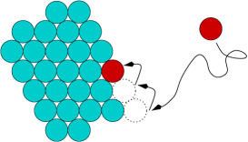
FIG. 3.: Illustration of the local relaxation process when an adatom arrives at an island edge.

contact with at least one nearest neighbor after a jump, is immediately transferred to a nearest neighbor site, if it can increase its coordination number. This procedure is repeated until the atom can no longer increase its local coordination (see Fig. 3).

Interlayer diffusion of atoms deposited onto islands is hindered by the Ehrlich-Schwoebel barrier $\Delta E_{\rm S}$, which reduces the jump rate $D/6a^{2}$ by the edge crossing probability $\alpha=\exp(-\Delta E_{\rm S}/k_{\rm B}T)$.[40] For computational convenience, we model the crossing by a two-step process in the simulation: First, when an atom passes the boundary, it remains in the same layer but moves to a place, where it is supported by only two atoms underneath. Then the atom immediately drops down to the layer below and moves to the nearest “stable” site according to the local relaxation mechanism introduced above (for similar simulations including $\Delta E_{\rm S}$, see, e.g. [13, 41]). We do not distinguish between crossing of A and B steps and have not attempted to model any more realistic scenarios, as e.g. collective rearrangements of atoms including exchange processes.[42, 43, 44] This is well justified as long as one is interested in the influence of an effective Schwoebel barrier.[23]

In the following, we focus on the case $i\!=\!1$ first. Typical film morphologies resulting from the simulations have been shown in Fig. 2b. Note that the boundaries of the islands are still rough despite the local relaxation mechanism. The fraction $f(t)$ of covered islands as a function of the total coverage $Fa^{2}t$ is shown in Fig. 4 for some representative parameters (full symbols). As expected, $f(t)$ first is close to zero, then increases strongly in some time interval around a “critical time” $t_{c}$, and finally saturates at one. In the inset of Fig. 4 we show the dependence of the mean island radius $R(t)\!\equiv\!(\langle s(t)\rangle/\pi)^{1/2}a$ on $Fa^{2}t$ during the evaporation. In agreement with eq. (18), we find $R(t)=A(Fa^{2}t)^{1/2}\Gamma^{1/6}$ with $A\!\cong\!0.78$.

To be specific, let us define the critical time $t_{c}$ via the condition $f(t_{c})\!=\!1/2$, and the corresponding critical island radius $R_{c}$ by $R_{c}\!=\!R(t_{c})$,

$$f(t_{c})=1/2\,,\hskip 4.26773ptR_{c}\equiv R(t_{c})=A(Fa^{2}t_{c})^{1/2}\Gamma^{i/2(i\!+\!2)}a\,.$$ (26)

Plots of $R_{c}$ as a function of $\alpha$ for various fixed $\Gamma$ are shown in Fig. 5 (full symbols). With increasing step edge barrier, i.e. decreasing $\alpha$, adatoms on average remain longer

FIG. 4.: The fractions $f(t)$ (full symbols) and $f_{0}(t/1.21)$ (open symbols) of covered island as a function of the total coverage $Fa^{2}t$ for $i\!=\!1$, $\alpha\!=\!10^{-5}$, and three different $\Gamma\!=\!10^{5}$ ($\scriptscriptstyle\blacksquare$, $\scriptscriptstyle\square$), $10^{6}$ ($\bullet$, $\circ$), and $10^{7}$ ($\blacktriangle$, $\triangle$). The dashed lines fitting $f_{0}(t/1.21)$ were calculated from the theoretical predictions for the second layer nucleation rate $\Omega(R(t))$ (eq. (42)). The solid lines fitting $f(t/1.21)$ were calculated according to eq. (29) with $\chi_{\sigma}(\sigma)\!\sim\!\sigma^{2}$ (see text). The inset displays the time-dependence of the mean island radius $R(t)\!\equiv\!(\langle s(t)\rangle/\pi)^{1/2}a$ (see eqs. (7,18)).

FIG. 5.: Dependence of the critical island radius $R_{c}$ on $\alpha$ for $i\!=\!1$ and various $\Gamma=10^{5}$ ($\scriptscriptstyle\blacksquare$, $\scriptscriptstyle\square$), $10^{6}$ ($\bullet$, $\circ$), $10^{7}$ ($\blacktriangle$, $\triangle$), and $10^{8}$ ($\blacktriangledown$, $\triangledown$). Full symbols refer to the results from the multi-island model, while open symbols refer to the results obtained from the single-island model ($R_{c}=1.1R_{c}^{\prime}$). The dashed line marks the onset of layer-by-layer growth, and the solid line with negative slope marks the crossover between regimes I and II; the solid lines fitting the data in regime II have slope 1/7.

on an island and nucleation of stable dimers occurs at smaller island radii. Accordingly, $R_{c}$ decreases with decreasing $\alpha$ (see “regime II” in the figure). For very small $\alpha$, however, the step edge barrier is practically never surmounted and thus is in effect infinitely high. Therefore, $R_{c}$ becomes independent of $\alpha$ (“regime I” in Fig. 5). The crossover between the two regimes is marked by the thick solid line. The full symbols in Fig. 5 terminate at the dashed line $\alpha_{\star}(\Gamma)$, which marks the onset of island coalescence. For $\alpha\!>\!\alpha_{\star}(\Gamma)$, islands in the first layer merge before second layer nucleation takes place and $R_{c}$ can no longer determined from the multi-island model. It is important to note that the dependence of $R_{c}$ on $\alpha$ is much weaker than predicted by the TDT approach: The solid lines in regime II have slope 1/7 corresponding to a power law $R_{c}\sim\alpha^{1/7}$ rather than $R_{c}\sim\alpha^{1/3}$ as predicted by eqs. (23, 25). Moreover, regime I does not occur in the TDT approach.

B Single-island model

Second layer nucleation can also be addressed in a simpler model, which does not attempt to describe the entire growth dynamics, but focuses on the decisive factors that determine nucleation in the presence of the step-edge barrier. In this model the complicated nucleation and diffusion-mediated growth of the two-dimensional islands, on which the second layer nucleation takes place, is replaced by letting the radius of one circular island expand deterministically in time as $R(t)/a\!=\!A(Fa^{2}t)^{1/2}\Gamma^{i/2(i\!+\!2)}$, where $A$ is taken from the full simulation of the multi-island model.

The island is embedded in a substrate area large enough to accommodate the island at all relevant times. Deposition and diffusion of adatoms take place in the same manner as in the multi-island model. Atoms inside the island boundary can escape by overcoming the step edge barrier. Those atoms that have surmounted the barrier or that have been deposited outside the island boundary are removed from the lattice. Thus the single-island model considers the deposition of random walkers within a time-dependent, circular boundary that is partially reflecting. Due to its greater simplicity, it allows for more specific analysis with a larger parameter space (there is no restriction due to coalescence of distinct islands).

In the non-interacting particle model, the “critical event” is to find $(i\!+\!1)$ atoms on neighboring lattice sites. Analogous to the multi-island model we can define the fraction $f_{0}(t)$ of covered islands up to time $t$. The fraction now refers to a set of islands obtained in independent simulation runs. All islands in these runs grow with the same deterministic growth law. Results for $f_{0}(t)$ are shown in Fig. 5 (open symbols) for the same parameters as in the multi-island model. Good agreement with $f(t)$ is achieved for small times (corresponding to $f(t)\!\lesssim\!1/2$), when the time in the single-island model is rescaled by a constant factor, i.e. $f(t)\!\simeq\!f_{0}(t^{\prime})$ with $t^{\prime}\!=\!t/1.21$. The factor is a consequence of the idealized circular island perimeter in the single-island model. In the multi-island model by contrast, the islands are far from being perfectly circular (see Fig. 2). They have rougher edges with more boundary sites, which causes adatoms to escape the islands more easily and second layer nucleation to occur at later times $t\!\cong\!1.21t^{\prime}$.

At larger times (corresponding to $f(t)\!\gtrsim\!1/2$), however, $f(t)$ deviates from $f_{0}(t^{\prime})$ and these deviations become more pronounced for larger $\Gamma$. The reason for this discrepancy is the presence of islands with size much smaller than $\langle s(t)\rangle$ in the multi-island model. Nucleation of stable clusters on top of these islands occurs at a later time, which causes $f(t)$ to be smaller than $f_{0}(t^{\prime})\!=\!f_{0}(t/1.21)$ at large $t$. In fact, we will show in Sec. III C that this effect can be accounted for by considering the probability distribution of islands with a certain size and capture area. When $R_{c}$ approaches the mean distance $l$, coalescences of larger islands also lead to modifications of $f(t)$ for $t\gtrsim t_{c}$.

The critical radius $R_{c}^{\prime}$ in the single-island model can be defined as in the many island model by $R_{c}^{\prime}\!=\!R(t_{c}^{\prime})$, where $f_{0}(t_{c}^{\prime})\!=\!1/2$. Due to the fact that $t_{c}\!=\!1.21t_{c}^{\prime}$ we expect $R_{c}\!=\!1.21^{1/2}R_{c}^{\prime}\!=\!1.1R_{c}^{\prime}$. Results for $1.1R_{c}^{\prime}$ as a function of $\alpha$ are shown in Fig. 5 (open symbols) for the same parameters as in the multi-island model (full symbols). As can be seen from the figure, there is almost perfect agreement between both data sets. Moreover, the data for $R_{c}^{\prime}$ can be obtained also beyond the dashed line marking the onset of layer-by-layer growth. Let us also note that, as long as one is interested only in $R_{c}^{\prime}$ (or $R_{c}=1.1R_{c}^{\prime}$), one may obtain it even more simply in the single-island model (without calculating $f_{0}(t)$) by determining the average radius of the island at the time of the nucleation event,

$$R_{c}^{\prime}=R(t_{c}^{\prime})\simeq\int_{0}^{\infty}dt\,\frac{df_{0}(t)}{dt}\,R(t)\,.$$ (27)

Note that $df_{0}(t)/dt$ is the probability density of the second layer nucleation times and that the average of $R(t)$ with respect to $df_{0}(t)/dt$ is approximately equal to $R(t_{c}^{\prime})$, since $df_{0}(t)/dt$ is sharply peaked around $t_{c}^{\prime}$.

C Equivalence of the single-island and the multi-island model

In order to determine $f(t)$ from $f_{0}(t)$ we define by $\psi(s,\sigma,t)\,ds\,d\sigma$ the probability for an island to have a size in the interval $[s,s\!+\!ds]$ and a capture area in the interval $[\sigma,\sigma\!+\!d\sigma]$ at time $t$, where the capture area is given by the Voronoi cell associated with an island.[25]

Let us consider $f_{0}(t)$ to be a functional of the growth law $R(t)$ only, as it is the case, for example, when one approximates the second layer nucleation by a Poisson process with a time dependent nucleation rate $\Omega(R(t))$. Then $f_{0}(t)=G_{0}[R(t)]=1-\exp[-\int_{0}^{t}dt^{\prime}\,\Omega(R(t^{\prime}))]$ (see eq. 17). In the saturation regime the growth law for an island can be written as $\pi R^{2}(t)=s_{\times}+F\sigma(t-t_{\times})$, where $t_{\times}$ is the time when the saturation is reached (see Fig. 1) and $s_{\times}$ is the island size at that time. (We restrict ourselves to film-morphologies far from coalescence here, so that $\sigma$ can be regarded as time-independent.) With the specified growth law, the functional $G_{0}[R(t)]$ can be expressed by a function $g_{0}=g_{0}(t;s_{\times},\sigma,t_{\times})$, and $f(t)$ is calculated via

$$f(t)=\int_{0}^{\infty}ds_{\times}\int_{0}^{\infty}d\sigma\,\psi(s_{\times},\sigma,t_{\times})\,\,g_{0}(t;s_{\times},\sigma,t_{\times})\,.$$ (28)

A detailed investigation of the probability distribution $\psi(s,\sigma,t)$ is certainly of interest but beyond the scope of the present work. A simple idea would be to neglect correlations between the stochastic variables $s$ and $\sigma$, $\psi(s,\sigma,t)\simeq\chi_{s}(s,t)\chi_{\sigma}(\sigma,t)$, and to use previously derived scaling forms for the island size distribution $\chi_{s}(s,t)$ (see e.g. refs. [35, 24]) and the capture area distribution $\chi_{\sigma}(\sigma,t)$ (see e.g. refs. [29, 45]).

Here we will follow a simpler approach. Since for typical situations we find both $s_{\times}$ and $t_{\times}$ to be significantly smaller than $s_{c}\!=\!\pi R_{c}^{2}$ and $t_{c}$, respectively, we use the growth law $s(t)\!=\!F\sigma t$ for an island with capture area $\sigma$ in the full simulation. The on-top nucleation probabilities $\tilde{g}_{0}(t;\sigma)$ for islands exhibiting different capture areas can then be related by a rescaling of time, i.e. $\tilde{g}_{0}(t;\sigma_{1})=\tilde{g}_{0}(\sigma_{1}t/\sigma_{2};\sigma_{2})$. Moreover, since for film morphologies far from coalescence ($\alpha\ll\alpha_{\star}(\Gamma)$), $\chi(\sigma,t)$ is approximately independent of time, we have $f_{0}(t)\!=\!\tilde{g}_{0}(t;\bar{\sigma})$, where $\bar{\sigma}\!=\!\int d\sigma\chi_{\sigma}(\sigma,t)\sigma\!\simeq\!\rho_{x}^{-1}$. Hence,

$$f(t)\!=\!\int_{0}^{\infty}d\sigma\,\chi_{\sigma}(\sigma)\,\tilde{g}_{0}(t;\sigma)=\int_{0}^{\infty}d\sigma\,\chi_{\sigma}(\sigma)\,f_{0}\Bigl{(}\frac{\bar{\sigma}}{\sigma}t\Bigr{)}\,.$$ (29)

In this simplified eq. (29) knowledge of the nucleation rate $\Omega(R)$ is not necessary and $f(t)$ can be directly obtained from $f_{0}(t)$ when $\chi_{\sigma}(\sigma)$ is known.

Writing $\chi_{\sigma}(\sigma)\!=\!\bar{\sigma}^{-1}h(\sigma/\bar{\sigma})$, where $\int dx\,h(x)\!=\!\int dxh(x)x\!=\!1$, the transformation (29) becomes $f(t)\!=\!\int_{0}^{\infty}dxh(x)f_{0}(xt)$. For a random distribution of point islands, we would have $h(x)\!=\!\exp(-x)$. However, since there is a depletion zone of adatoms near an island, the probability for other islands to nucleate in an area close to an existing one is reduced and not exponential. For an isolated island, dimensional analysis predicts the extension $\xi$ of the depletion zone to be of order $(D/F)^{1/4}$. By comparing $\xi$ with the mean distance $l\sim\rho_{x}^{-1/2}\sim\Gamma^{i/2(i\!+\!2)}$ between islands, we expect that $h(x)$ exhibits a large $x$ regime with $h(x)\sim\exp(-x)$ only for $i\!>\!2$. For $i\!=\!1$ we thus are satisfied with a simple power law ansatz $h(x)\!=\!Cx^{\phi}$ for $x\leq x_{\star}$, where $C$ and $x_{\star}$ follow from the two conditions imposed on $h(x)$, and $\phi$ is a fitting parameter.

To test this ansatz we take $f_{0}(t)$ for $\Gamma\!=\!10^{7}$ from Fig. 4 (open symbols or dotted lines) and compare $f(t)$ as calculated from eq. (29) (solid lines in Fig. 4) with the corresponding $f(t)$ as obtained in the simulation (full symbols in Fig. 4). As can be seen from Fig. 4, for $\Gamma\!=\!10^{6}$ and $\Gamma\!=\!10^{7}$ a fairly good account of the differences between $f_{0}(t)$ and $f(t)$ can be obtained by choosing $\phi\!=\!2$. However, for $\Gamma\!=\!10^{5}$ the theoretical curve underestimates the fraction of covered islands at large times (where $f(t)\gtrsim 1/2$). Better agreement between theory and simulation can only be obtained if one would allow $\phi$ to depend on $\Gamma$. Alternatively, we have tried an ansatz for $h(x)$ similar to that used by Amar and Family for the scaling function characterizing the island size distribution (see eq. (8)). This ansatz yields comparable results, but is also not successful in accounting for the changes with $\Gamma$. We finally have to note, that at the time when submitting the paper, a more detailed theoretical account for $\psi(s,\sigma,t)$ was published.[46] The use of this finding in eq.(28) and the comparison of the resulting $f(t)$ with Monte Carlo data will be presented elsewhere.

Having shown that the single-island and multi-island models are essentially equivalent, except for differences between $f(t)$ from $f_{0}(t)$ for large times that can be attributed to the island size distribution, we will focus on the single-island model in the remaining part of the paper.

IV Second layer nucleation in simple situations

In this Section we develop a stochastic description of the nucleation process based on the scaling approach for second layer nucleation presented in ref. [16] (see also ref. [17]). The procedure focuses on the non-interacting particle model, although formally it is possible to extend scaling concepts also to situations, where the lifetimes of unstable clusters become important. This was shown by Krug et al.[17] and is discussed in a more general context in Sec. IV E. The treatment of the non-interacting particle model outlined in Sec. IV A already captures the salient features of the problem in terms of lifetimes, occupation probabilities and encounter rates. We will show that there exist two possible mechanisms for the formation of a stable cluster: In the first case, there is typically no atom on top of the island and a stable cluster is formed due to fluctuations, in which by chance $i\!+\!1$ atoms are present on the island. In the second case by contrast, there are on average more than $i\!+\!1$ atoms on top of the island during the formation of a stable cluster so that the nucleation process can be described in a mean-field type manner.

It turns out that the fluctuation-dominated case takes place for $i\!\leq\!2$, while the mean-field situation occurs for $i\!\geq\!3$. The TDT approach corresponds to the mean-field case with the notable supplement that for very large step edge barriers one should deal with the time-dependent adatom density $\rho_{1}(r,t)$ (solution of eqs. (9,10)) to calculate the nucleation rate $\Omega(R)$ from eq.(16). In the language of critical phenomena, one may regard $i\!=\!2$ as the upper critical size of the critical nucleus above which mean-field theory becomes applicable. We have to note that the existence of this upper critical size was not perceived by us in ref. [16], and accordingly, the extension of the scaling arguments for the fluctuation-dominated situation to $i\!=\!3$ was not allowed.

In the stochastic formulation presented below we will develop many of the necessary ingredients for the general treatment of second layer nucleation in the next Sec. V. Moreover, it is discussed under which conditions mean-field type expressions $\propto D\rho_{1}^{i+1}$ for local nucleation rates can be used.

A General procedure

In order to determine a second layer nucleation rate $\Omega(R)$ we start by considering a time interval $\Delta t(R)$, during which $R(t)$ does not change significantly. For example, for the generic growth law (18) we may require $\Delta t(R)$ to correspond to a 10% change of $R$, which would give $\Delta t(R)=0.21(R/a)^{2}/[A^{2}Fa^{2}\Gamma^{i/(i\!+\!2)}]$, i.e.

$$\Delta t(R)\sim F^{-1}\Gamma^{-i/(i\!+\!2)}R^{2}$$ (30)

The nucleation rate $\Omega(R)$ is the mean number $n_{\scriptscriptstyle\rm nuc}(R)$ of nucleation events in time $\Delta t(R)$ divided by $\Delta t(R)$,

$$\Omega(R)=\frac{n_{\scriptscriptstyle\rm nuc}(R)}{\Delta t(R)}\,.$$ (31)

A nucleation event occurs, if $i\!+\!1$ atoms encounter each other on nearest neighboring sites.

For an island with radius $R$ and infinite step edge barrier ($\alpha=0$), and in total $n$ single atoms on top of it, let us approximate the encounter dynamics by a Poisson process, where $\omega_{n}(R)$ denotes the encounter rate of exactly $i\!+\!1$ atoms. Within the Poisson approximation this rate can be precisely defined as the inverse average time for $i\!+\!1$ atoms to encounter each other for the first time, when initially $n$ atoms are randomly distributed on top of the island. A simple scaling argument yields

$$\omega_{n}(R)=\kappa_{\rm e}\,\left[\prod_{k=0}^{i}(n\!-\!k)\right]\,\frac{D}{a^{2}}\,\left(\frac{a^{2}}{\pi R^{2}}\right)^{i\!+\!1}\,\frac{\pi R^{2}}{a^{2}}\,,$$ (32)

where $\kappa_{\rm e}$ is a constant. The term $(a^{2}/\pi R^{2})^{i\!+\!1}$ is proportional to the probability to find $i\!+\!1$ atoms on nearest neighbor sites, and the factor $(\pi R^{2}/a^{2})$ takes into account that the encounter can occur everywhere on the island. The combinatorial factor $\prod_{k=0}^{i}(n\!-\!k)$ is slightly more subtle. At first sight, one may think that one should include the number ${n\choose i\!+\!1}$ of possibilities to choose any $i\!+\!1$ atoms out of the $n$ atoms but this is not correct, since the accumulation of $i\!+\!1$ atoms does not happen “in parallel” at a certain instant of time but in order: First a dimer forms out of $n$ single atoms (combinatorial factor $n(n\!-\!1)/2$) and then some of the remaining $n\!-\!k$ atoms ($k\!=\!2,3,\ldots,i$) have to attach one after another to an intermediate cluster of size $k$ before this cluster dissociates (the intermediate cluster is assumed to be much less mobile than single adatoms). The sequential attachment process yields an additional combinatorial factor $\prod_{k=2}^{i}(n\!-\!k)$. Clearly, the scaling argument gives only a

FIG. 6.: Scaled rate $\omega_{n}(R)(a^{2}/D)/\prod_{k=0}^{i}(n\!-\!k)$ of the encounter of $i\!+\!1$ atoms out of $n$ atoms on an island with radius $R$ and infinite step edge barrier. The upper curve with slope (-2) refers to $i\!=\!1$ and $n\!=\!2$ ($\scriptscriptstyle\square$), 3 ($\circ$), and 4 ($\triangle$), and the lower curve with slope (-4) refers to $i\!=\!2$ and $n\!=\!3$ ($\triangledown$), 4 ($\lozenge$), and 5 ($\times$).

rough approximation for $\omega_{n}(R)$ and a more refined treatment justifying eq. (32) is presented in Appendix A.

Determination of $\omega_{n}(R)$ for $i\!=\!1,2$ and various $n$ in our simulations confirms the behavior predicted by eq. (32), see Fig. 6. For $i\!=\!1$ the scaling law is only valid for large $R\!\gtrsim\!100a$, because at smaller $R$, two atoms typically encounter each other before the delta-functions characterizing the initial occupancy smear out to a uniform distribution (for larger $i$ this effect becomes less important). Moreover, we find $\kappa_{\rm e}\!\cong\!0.087$ for $i\!=\!1$ and $\kappa_{\rm e}\!\cong\!0.53$ for $i\!=\!1$, i.e. the coefficient $\kappa_{\rm e}$ is constant for fixed $i$, but changes strongly with $i$. This dependence is expected, since we neglected the memory effect that, when $n$ atoms, $2\!\leq\!n\!\leq\!i$, are already close to each other, they keep close together for a while so that the encounter of $i\!+\!1$ atoms during this intermediate time becomes more likely. This memory effect is not included in the treatment in Appendix A, where after each “dissociation” of an unstable cluster of size $k\!\leq\!i$ a configuration is assumed to emerge, where a cluster of size $k\!-\!1$ is left and the remaining $n\!-\!k$ atoms are assumed to be randomly distributed. Accordingly, $\kappa_{\rm e}$ should increase with increasing $i$ as it is the case.

Equation (32) has been derived for an infinite step edge barrier. For finite step edge barriers, we have to take into account that a state corresponding to an island with $n$ atoms on top of it has a finite lifetime $\tau_{n}(R)$ only. This lifetime is defined by the average time required for the first of the $n$ atoms to escape from the island (if any encounter processes are neglected). To a good approximation, $\tau_{n}(R)$ is the $n$th fraction of the lifetime $\tau_{1}(R)$ of a single atom, $\tau_{n}(R)\!\simeq\!\tau_{1}(R)/n$ (this approximation would become exact, if the escape were a simple Poisson process). In the limit of large $\alpha$, $\tau_{1}(R)$ is proportional to the characteristic time $R^{2}/D$ for an atom to reach the boundary, while for small $\alpha$ an atom typically returns many times to the boundary before escaping from the island. Thus, in the latter limit, the characteristic escape rate (inverse lifetime $\tau_{1}^{-1}$) is approximately given by the product of the probability $2\pi Ra/\pi R^{2}$ for the atom to be at the boundary and the rate $\alpha D/6a^{2}$ to overcome the step edge barrier. Combining these results gives

$$\tau_{n}(R)=\frac{1}{n}\,\frac{R^{2}}{D}\,\left(\kappa_{1}\frac{a}{\alpha R}+\kappa_{2}\right)\,,$$ (33)

where $\kappa_{1}$ and $\kappa_{2}$ are constants. Indeed, an exact solution of the corresponding diffusion problem [47] allows one to derive $\tau_{n}(R)$ exactly in the continuum limit, as we have shown in Appendix B. In particular, when the escape is approximated by a Poisson process, one finds $\kappa_{1}\!\cong\!1$ and $\kappa_{2}\!=\!1/2$ after proper renormalization and taking into account the lattice corrections (see Appendix B). Direct determination of $\tau_{1}(R)$ in our simulations confirms this result, see Fig. 7.

Knowing $\tau_{n}(R)$ we can calculate the probability $p_{n}(R)\!=\!p_{n}(R(t))$ to find exactly $n$ atoms on top of the island at time $t$ before onset of second layer nucleation. This is achieved by considering the time evolution of $p_{n}(R(t))$, which is described by the master equation

$$\frac{dp_{n}}{dt} = \pi FR(t)^{2}\,\bigl{[}(1\!-\!\delta_{n,0})p_{n-1}-p_{n}\bigr{]}$$ (35)

$${}+\bigl{[}\frac{p_{n+1}}{\tau_{n+1}(R(t))}-\frac{p_{n}}{\tau_{n}(R(t))}\bigr{]}$$

with the initial condition $p_{n}(0)\!=\!\delta_{n,0}$. Note that we have formally introduced $p_{-1}$ and that $1/\tau_{n}\!\propto\!n$ so that the last term on the right hand side of (35) does not contribute for $n\!=\!0$. As can be expected and is explicitly shown in Appendix B, the solution of eq. (36) is the Poisson distribution

$$p_{n}(R)=\frac{\bar{n}(R)^{n}}{n!}\exp[-\bar{n}(R)]\,,$$ (36)

where the mean number $\bar{n}(R)$ of atoms on top of the

FIG. 7.: Lifetime $\tau_{1}(R)$ of a single atom on an island with radius $R$ in units of $a^{2}/D$ for various edge crossing probabilities $\alpha\!=\!\exp(-\Delta E_{\rm S}/k_{\rm B}T)$. The solid lines are drawn according to eq. (33) with $\kappa_{1}\!=\!1$ and $\kappa_{2}\!=\!1/2$.

island before onset of nucleation is

$$\bar{n}(R)=\frac{2\pi}{A^{2}\Gamma^{\scriptstyle\frac{i}{i\!+\!2}}}(1\!+\!\tilde{\alpha}R)^{-\varphi}\int_{0}^{R}dx\,x^{3}\,(1\!+\!\tilde{\alpha}x)^{\varphi}\,.$$ (37)

Here $\tilde{\alpha}\!\equiv\!\kappa_{2}\alpha/\kappa_{1}$ and $\varphi\!\equiv\!2A^{-2}\Gamma^{2/(i\!+\!2)}/\kappa_{2}$. An explicit solution after evaluating the integral in eq. (37) is given in eq. (B19) of Appendix B. For fixed $\alpha$ and $\Gamma$, three distinct $R$ regimes can be identified from eq. (37): For $\varphi\tilde{\alpha}R\ll 1$ we can use $(1\!+\!\tilde{\alpha}x)^{\varphi}\!\simeq\!1$ in (37), while for $\alpha R\ll 1$ but $\varphi\tilde{\alpha}R\gg 1$ we can use $(1\!+\!\tilde{\alpha}x)^{\varphi}\!\simeq\!\exp(\varphi\tilde{\alpha}x)$. For $\tilde{\alpha}R\!\gg\!1$, we can set $(1\!+\!\tilde{\alpha}R)\!\simeq\!\tilde{\alpha}R$ in (37), and, since the integral over $x$ is dominated by the upper bound, $(1\!+\!\tilde{\alpha}x)\!\simeq\!\tilde{\alpha}x$ also. We thus obtain

$$\bar{n}(R)\sim\left\{\begin{array}[]{l@{\hspace*{0.2cm}}l}\Gamma^{-i/(i\!+\!2)}R^{4}\,,\hfil\hskip 5.69046pt&R/a\!\ll\!\Gamma^{-2/(i\!+\!2)}\alpha^{-1}\\[5.69046pt] \Gamma^{-1}\alpha^{-1}R^{3}\,,\hfil\hskip 5.69046pt&\Gamma^{-2/(i\!+\!2)}\alpha^{-1}\!\ll\!R/a\!\ll\!\alpha^{-1}\\[5.69046pt] \Gamma^{-1}R^{4}\,,\hfil\hskip 5.69046pt&\alpha^{-1}\!\ll\!R/a\end{array}\right.$$ (38)

The two regimes for large $R$ correspond to a quasi-stationary situation ($dp_{n}/dt\!=\!0$ in eq. (35)), where $p_{n}(R)$ from eq. (36) equals the stationary distribution for $R\!=\!R(t)$ with $\bar{n}(R)\!=\!\pi FR^{2}\tau_{1}(R)$. In these regimes the same result (38) can be obtained also by integrating $\rho_{1}^{\scriptscriptstyle\rm st}$ from eq. (11) over the island area. In fact, we used this connection to renormalize the constants $\kappa_{1}$ and $\kappa_{2}$ in eq. (33), see Appendix B. The small $R$ regime in eq. (38) corresponds to a non-stationary situation, where $p_{n}$ in general depends on the function $R(t^{\prime})$ at all times $0\!\leq\!t^{\prime}\leq t$ and not only on its value $R(t)$ at time $t^{\prime}\!=\!t$. This fact, however, which also concerns the crossover value $R_{\times}\!\sim\!\Gamma^{-2/(i\!+\!2)}\alpha^{-1}$ to the non-stationary regime, is of minor importance here, since we consider the generic growth law (18) throughout the paper. We thus can use $R$ and $t$ interchangeably. Note that the crossover from the non-stationary to the quasi-stationary situation occurs when $\tau_{1}(R_{\times})\sim\Delta t(R_{\times})$, that means in the non-stationary small $R$ regime the changes in the radius occur on a faster scale than the escape of an atom from the island, $\Delta t(R)\ll\tau_{1}(R)$, while in the two quasi-stationary large $R$ regimes $\Delta t(R)\gg\tau_{1}(R)$.

Let us now return to the different scenarios discussed in the introductory part of this Section. When $\bar{n}(R)\gtrsim i\!+\!1$, nucleation of a stable cluster can take place at any instant of time. The number of nucleations in $\Delta t(R)$ that result from states with exactly $n$ atoms on top of the island is proportional to $\omega_{n}(R)\Delta t(R)$. The total number $n_{\scriptscriptstyle\rm nuc}(R)$ is the weighted sum of $\omega_{n}(R)\Delta t(R)$ over $n$, i.e. we find $n_{\scriptscriptstyle\rm nuc}(R)\!=\!\sum_{n=i\!+\!1}^{\infty}p_{n}(R)\omega_{n}(R)\Delta t(R)$ (we are allowed to extend the sum up to infinity due to the sharp decrease of the Poisson distribution for $n\!\gg\!\bar{n}(R)$). With eq. (31) we thus obtain for the mean-field nucleation rate

$$\Omega_{\scriptscriptstyle\rm mf}(R) = \sum_{n=i\!+\!1}^{\infty}p_{n}(R)\,\omega_{n}(R)$$ (39)

$$= \kappa_{\rm e}\,\frac{D}{a^{2}}\left(\frac{\bar{n}(R)}{\pi R^{2}}a^{2}\right)^{i\!+\!1}\left(\frac{\pi R^{2}}{a^{2}}\right)\,.$$ (40)

Equation (40) can be interpreted as resulting from a local nucleation rate $\propto D\rho_{1}^{i\!+\!1}\!=\!D[\bar{n}(R)/\pi R^{2}]^{i\!+\!1}$ integrated over the island area (factor $\pi R^{2}$). Compared to the TDT approach the radial variation of the diffusion profile $\rho_{1}\!=\!\rho_{1}(r)$ is neglected in the stochastic description, so that $\Omega(R)$ from eq. (16) may be preferred over eq. (40).[48] However, as will be discussed further in Sec. IV D below, for large $\alpha$ one should use the non-stationary solution of eqs. (9,10) for calculating $\Omega(R)$ from (16) corresponding to the small $R$ regime of $\bar{n}(R)$ in eq. (38).

More important, eq. (40) (or (16)) can be used only if $\bar{n}(R_{c})\gtrsim i\!+\!1$ in the relevant time interval $\Delta t(R_{c})$ at the onset of second layer nucleation. The stochastic description allows us to treat also the fluctuation dominated case, where $\bar{n}(R_{c})\ll i\!+\!1$. In this situation $i\!+\!1$ adatoms have to be deposited and to encounter each other on the island. We can restrict our consideration to the deposition of exactly $i\!+\!1$ atoms, since for $\bar{n}(R_{c})\ll i\!+\!1$, fluctuations corresponding to more than $i\!+\!1$ atoms on the island occur with a probability $\sum_{n=i\!+\!2}^{\infty}p_{n}(R)\!<\!\exp(1)p_{i+1}(R)\bar{n}(R)/(i\!+\!2)\ll p_{i+1}(R)$. If an atom is deposited on the island already containing $i$ atoms, we view this as the start of a nucleation trial. The number $n_{\scriptscriptstyle\rm tr}(R)$ of nucleation trials in time $\Delta t(R)$ is $n_{\scriptscriptstyle\rm tr}(R)\!=\!\pi FR^{2}\Delta t(R)p_{i}(R)$. For a trial to be successful, the $i\!+\!1$ atoms on the island right after its start have to encounter each other before any of the atoms escapes by passing the step-edge barrier. The probability $p_{\scriptscriptstyle\rm enc}(R)$ for this to happen is

$$p_{\scriptscriptstyle\rm enc}(R)=1\!-\!\exp[-\omega_{i\!+\!1}(R)\tau_{i\!+\!1}(R)]\,.$$ (41)

Accordingly, the total number $n_{\scriptscriptstyle\rm nuc}(R)$ of nucleation events in time $\Delta t(R)$ is now $n_{\scriptscriptstyle\rm nuc}(R)\!=\!n_{\scriptscriptstyle\rm tr}(R)p_{\scriptscriptstyle\rm enc}(R)$, and using eq. (31) we obtain for the fluctuation-dominated nucleation rate

$$\Omega_{\scriptscriptstyle\rm fl}(R) = \pi FR^{2}\,p_{i}(R)\,p_{\scriptscriptstyle\rm enc}(R)$$ (42)

$$= \pi FR^{2}\frac{\bar{n}(R)^{i}}{i!}e^{-\bar{n}(R)}\Bigl{(}1\!-\!\exp[-\omega_{i\!+\!1}(R)\tau_{i\!+\!1}(R)]\Bigr{)}\,.$$ (43)

We note that in both formulae (40,42) the only parameter not known a priori is the coefficient $\kappa_{\rm e}$, which has to be taken from simple simulations of the encounter process (see Fig. 6 and the discussion above). Hence they do not require more input parameters than the expression (16) resulting from the TDT approach.

It remains to clarify, when the mean-field or the fluctuation dominated situation occurs, i.e. when $\Omega_{\scriptscriptstyle\rm mf}(R)$ or $\Omega_{\scriptscriptstyle\rm fl}(R)$ has to be used as second layer nucleation rate. The answer to this question can be found by self-consistency requirements: Suppose first that the fluctuation dominated case takes place. Then, using (42), one can calculate the critical radius $R_{c}$ and check if the condition $\bar{n}(R_{c})\!\ll\!i\!+\!1$ is fulfilled. In addition the condition $\omega_{i+1}(R_{c})\Delta t(R_{c})\!\gtrsim\!1$ should be fulfilled too, since the encounter of $i\!+\!1$ atoms in the characteristic time $\omega_{i+1}(R_{c})^{-1}$ should happen before $R_{c}$ changes. If these necessary conditions for the fluctuation-dominated case are obeyed, then the mean-field situation is ruled out. This conclusion can be drawn, since $\bar{n}(R)$ is monotonously increasing with $R$, which implies that $R_{c}$ following from $\Omega_{\scriptscriptstyle\rm fl}(R)$ is always smaller than $R_{c}$ resulting from $\Omega_{\scriptscriptstyle\rm mf}(R)$. Hence, when the fluctuations are likely enough to initiate second layer nucleation, they lead to the formation of stable clusters at an earlier time $t_{c}$ than that expected from the mean-field approach.

We will now show that the fluctuation-dominated case occurs for $i\!=\!1,2$. The detailed analysis is a bit technical and the reader, who is interested in the main findings only, may skip the discussion of the various regimes I-IV in the following subsection and proceed with the summary of the results given right after this discussion.

B Small critical nuclei ($i\!=\!1,2$)

Using $\Omega_{\scriptscriptstyle\rm fl}(R)$ from eq. (42) we can determine the critical radius $R_{c}$ (or, more precisely, $R_{c}^{\prime}$) by calculating $f_{0}(t)$ as in the TDT approach (see eq. (17)). However, for discussing the scaling of $R_{c}$ with $\Gamma$ and $\alpha$, it is easier to obtain $R_{c}$ from the condition

$$\Omega_{\scriptscriptstyle\rm fl}(R_{c})\Delta t(R_{c})\simeq 1\,,$$ (44)

which expresses the fact that the probability of second layer nucleation in $\Delta t(R_{c})$ becomes of the order of one. Since we consider the fluctuation-dominated case for small critical nuclei here ($i\!=\!1,2$), we assume $\bar{n}(R_{c})\!\ll\!1$ and thus set $\exp[-\bar{n}(R_{c})]\!\simeq\!1$, when inserting $\Omega_{\scriptscriptstyle\rm fl}(R_{c})$ from eq. (42) into eq. (44).

Four different regimes are then predicted by eq. (44):

• In the limit $\alpha\!\to\!0$ we have $\bar{n}(R)\!\sim\!\Gamma^{-i/(i\!+\!2)}R^{4}$ and $\tau_{i\!+\!1}\!\to\!\infty$. Hence we obtain from eqs. (30,42,44) $FR_{c}^{2}\Gamma^{-i^{2}/(i\!+\!2)}R_{c}^{4i}F^{-1}\Gamma^{-i/(i\!+\!2)}R_{c}^{2}\!\sim\!R_{c}^{4(i\!+\!1)}\Gamma^{-i(i\!+\!1)/(i\!+\!2)}\!\sim\!{\rm const.}$, i.e.

  $$R_{c}\sim\Gamma^{i/[4(i\!+\!2)]}$$ (45)

  From (45) follows $\bar{n}(R_{c})\sim{\rm const.}$, which means that the assumption of a fluctuation-dominated situation is not necessarily justified. In fact, eq. (45) appears here as the result of a rather lengthy calculation, but in the limit $\alpha\!\to\!0$, the same scaling behavior (45) can be obtained very simply by calculating the average time needed for the deposition of $i\!+\!1$ atoms (see ref. [16]). Hence, despite $\bar{n}(R_{c})\!\simeq\!i\!+\!1$, eq. (45) gives the correct scaling behavior. However, eq. (45) predicts $\omega_{i+1}(R_{c})\Delta t(R_{c})\!\sim\!DR_{c}^{-2i}F^{-1}\Gamma^{-i/(i\!+\!2)}R_{c}^{2}\!\sim\!\Gamma^{-(i^{2}\!-\!i\!-\!4)/[2(i\!+\!2)]}$ and since $\Gamma\!=\!D/Fa^{4}\!\gg\!1$,[49] the inequality $\omega_{i+1}(R)\Delta t(R_{c})\!\gtrsim\!1$ becomes violated for $i\!\geq\!3$. For $i\!\geq\!3$ therefore, the condition $\omega_{i+1}(R_{c})\Delta t(R_{c})\!\sim\!1$ should be used for calculating $R_{c}$, and because this yields $\bar{n}(R_{c})\!>\!i\!+\!1$, one may alternatively use $\Omega_{\scriptscriptstyle\rm mf}(R_{c})\Delta t(R_{c})\simeq 1$ as the determining relation (see Sec. IV D).

• With increasing $\alpha$, for $i\!\leq\!2$, either the non-stationarity condition $\tau_{1}(R_{c})\!\gg\!\Delta t(R_{c})$ ($\bar{n}(R_{c})\!\sim\!\Gamma^{-i/(i\!+\!2)}R_{c}^{4}$ in eq. (42)) or the condition $\omega_{i+1}(R_{c})\tau_{i+1}(R_{c})\!\gg\!1$ ($p_{\scriptscriptstyle enc}\simeq 1$ in eq. (42)) breaks down first. Taking $R_{c}$ from eq. (45), the first condition implies $\alpha\!\ll\!\Gamma^{-(i\!+\!8)/[4(i\!+\!2)]}$, while the second implies $\alpha\!\ll\!\Gamma^{-i(2i\!-\!1)/[4(i\!+\!2)]}$. Since the first condition is more restrictive for $i\!\leq\!2$, regime I ceases to be valid when $\alpha$ becomes larger than $\Gamma^{-(i\!+\!8)/[4(i\!+\!2)]}$ and the quasi-stationarity situation is reached. In eq. (42) we now have to take $\bar{n}(R_{c})\!=\!\pi FR^{2}\tau_{1}(R)\!\sim\!\Gamma^{-1}\alpha^{-1}R^{3}$ (see eq. (38)) and it follows $\Omega_{\scriptscriptstyle\rm fl}(R_{c})\Delta t(R_{c})\!\sim\!\alpha^{-i}\Gamma^{-i(i\!+\!3)/(i\!+\!2)}R_{c}^{3i\!+\!4}\!\sim\!{\rm const.}$, i.e.

  $$R_{c}\sim\alpha^{i/(3i\!+\!4)}\Gamma^{i(i\!+\!3)/[(i\!+\!2)(3i+4)]}\,.$$ (46)

  Since $\bar{n}(R_{c})\!\sim\!(\Gamma^{-(i\!+\!8)/4(i\!+\!2)}\alpha^{-1})^{4/(3i+4)}\!\ll\!1$ the condition for a fluctuation-dominated situation is fulfilled, and since $\Delta t(R_{c})\!\gg\!\tau_{1}(R_{c})\!\simeq\!\tau_{i+1}(R_{c})$ and $\omega_{i+1}(R_{c})\tau_{i+1}(R_{c})\!\gg\!1$ the condition $\omega_{i+1}(R_{c})\Delta t(R_{c})\!\gtrsim\!1$ is obeyed too.

• By further increasing $\alpha$ we obtain $\omega_{i+1}(R_{c})\tau_{i+1}(R_{c})\!\ll\!1$ for $\alpha\!\gg\!\Gamma^{-i(i\!+\!3)(2i\!-\!1)/[2(i\!+\!2)(i^{2}\!+\!i\!+\!2)]}$. Hence we now have to use $p_{\scriptscriptstyle enc}\!\simeq\!\omega_{i+1}(R_{c})\tau_{i+1}(R_{c})$ when inserting eq. (42) into eq. (44) and find

  $$R_{c}\sim\alpha^{(i\!+\!1)/(i\!+\!5)}\Gamma^{i(i\!+\!3)/[(i\!+\!2)(i+5)]}\,.$$ (47)

  The condition $\bar{n}(R_{c})\!\sim\!\Gamma^{-1}\alpha^{-1}R_{c}^{3}\!\ll\!1$ requires $\alpha^{i\!-\!1}\!\ll\!\Gamma^{-(i^{2}\!+\!i\!-\!5)/(i\!+\!2)}$ and is fulfilled for $i\!=\!1$. For $i\!=\!2$, it is valid for $\alpha\!\ll\!\Gamma^{-1/4}\!\sim\!a/R_{c}$. The second requirement $\omega_{i+1}(R_{c})\Delta t(R_{c})\!\gtrsim\!1$ gives $\alpha^{i\!-\!1}\!\ll\!\Gamma^{-(i^{3}\!+\!2i^{2}\!-\!4i\!-\!5)/[(i\!+\!1)(i\!+\!2)]}$ and again is obeyed for $i\!=\!1$ and valid for $i\!=\!2$ as long as $\alpha\!\ll\!\Gamma^{-1/4}\!\sim\!a/R_{c}$.

• In this last regime $\alpha$ becomes larger than $a/R_{c}$, that means eq. (47) predicts the regime to occur for $\alpha\!\gg\!\Gamma^{-i/[2(i\!+\!2)]}$. Taking $\bar{n}(R_{c})\!\sim\!\Gamma^{-1}R_{c}^{4}$ from eq. (38) and $\omega_{i+1}(R_{c})\tau_{i+1}(R_{c})\!\sim\!R_{c}^{-2(i-1)}$ from eqs. (32,33), we find

  $$R_{c}\sim\Gamma^{i/[2(i\!+\!2)]}\,.$$ (48)

  We used $\omega_{i+1}(R_{c})\tau_{i+1}(R_{c})\!\ll\!1$ ($p_{\scriptscriptstyle\rm enc}(R_{c})\!\ll\!1$) to derive (48), which for $i\!=\!2$ is valid and for $i\!=\!1$ is obeyed when taking into account the prefactors (for $i\!=\!1$ $\omega_{i+1}(R_{c})\tau_{i+1}(R_{c})\!=\!\kappa_{\rm e}\kappa_{2}$). Moreover, eq. (48) gives $\bar{n}(R_{c})\sim\Gamma^{(i\!-\!2)/(i\!+\!2)}$, which is much smaller than one for $i\!=\!1$. For $i\!=\!2$, a decision on whether the fluctuation-dominated or the mean-field situation occurs would require a closer inspection of the prefactors. However, since for $\alpha\!\gg\!a/R_{c}$ one finds the same scaling (48) in the mean-field situation (see Sec. IV D), eq. (48) is valid in any case. The second condition $\omega_{i+1}(R_{c})\Delta t(R_{c})\!\gtrsim\!1$ is fulfilled for $i\!=\!1$, and for $i\!=\!2$ the situation again depends on the prefactors.

In summary we have found that the second layer nucleation for $i\!=\!1,2$ occurs due to various mechanisms in four distinct regimes I-IV: In regime I ($\alpha\!\ll\!\Gamma^{-(i\!+\!8)/[4(i\!+\!2)]}$), the nucleation takes place once $i\!+\!1$ have been deposited on the island, in regime II ($\Gamma^{-(i\!+\!8)/[4(i\!+\!2)]}\!\ll\!\alpha\!\ll\!\Gamma^{-i(i\!+\!3)(2i\!-\!1)/[2(i\!+\!2)(i^{2}\!+\!i\!+\!2)]}$) the loss of atoms becomes important and the nucleation takes place once the probability for finding $i\!+\!1$ atoms on the island at some time instant in $\Delta t(R)$ becomes of the order of one, in regime III ($\Gamma^{-i(i\!+\!3)(2i\!-\!1)/[2(i\!+\!2)(i^{2}\!+\!i\!+\!2)]}\!\ll\!\alpha\!\ll\!\Gamma^{-i/[2(i\!+\!2)]}$) the probability $p_{\scriptscriptstyle\rm enc}$ for the encounter of $i\!+\!1$ atoms during a nucleation trial has to be taken into account in addition to the probability for the occurrence of $i\!+\!1$ atoms, and in regime IV ($\alpha\!\gg\!\Gamma^{-i/[2(i\!+\!2)]}$) both the occurrence and encounter probability matter but these probabilities no longer depend on the step edge barrier. For convenient reference, we provide the exponents $\gamma$ and $\mu$ defined in eq. (23) and their corresponding ranges of validity in Table I. When comparing the scaling in the fluctuation-dominated situation with that predicted by eqs. (24,25) of the TDT approach it is remarkable that the same behavior is found in regime III and IV. We believe this to be caused by the fortunate circumstance that local nucleation rates of form $\propto D\rho_{1}^{i\!+\!1}$ might be effectively applicable even if the requirements for the mean-field situation are not fulfilled (see however [50]).

Moreover, we have to note that for $i\!=\!1$ the lower and upper crossovers $\alpha_{2}$ and $\alpha_{3}$ specifying regime III (see table I) both scale as $\Gamma^{-1/6}$. This is due to the fact that when $\omega_{i+1}(R_{c})\tau_{i+1}(R_{c})$ becomes less than one, we already obtain $\alpha\!\gg\!a/R_{c}$, which is the condition for regime IV. Nevertheless, due to the pronounced small $R$ corrections to eq. (32) for $i\!=\!1$ (see Fig. 6) both conditions $\omega_{i+1}(R_{c})\tau_{i+1}(R_{c})\!\ll\!1$ and $\alpha\!\ll\!a/R_{c}$ can be fulfilled in a small transient regime III. However, for $i\!=\!1$ this is no longer a true scaling regime, where a simple power law dependence of $R_{c}$ on $\Gamma$ and $\alpha$ can be identified. In this respect, the small $\alpha$ regime of the TDT approach does not occur for $i\!=\!1$, also not at larger $\alpha$.

C Comparison with simulations for i=1,2

Taking $\Omega_{\rm\scriptscriptstyle fl}$ from eq. (42) we can calculate $f_{0}(t)$ according to eq. (17). Representative results for $i\!=\!1$ are shown in Fig. 4 (solid lines), and the comparison with the Monte Carlo data yields a very good agreement. The $R_{c}$ values

TABLE I.: The exponents $\gamma$ and $\mu$ characterizing the scaling $R_{c}\!\sim\!\Gamma^{\gamma}\alpha^{\mu}$ in the various regimes I-IV for $i\!=\!1,2$

Regime	Rangea	$\gamma$	$\mu$
I	$0\!\leq\!\alpha\!\ll\!\alpha_{1}$	$i/4(i\!+\!2)$	0
II	$\alpha_{1}\!\ll\!\alpha\!\ll\!\alpha_{2}$	$i(i\!+\!3)/(i\!+\!2)(3i\!+\!4)$	$i/(3i\!+\!4)$
III	$\alpha_{2}\!\ll\!\alpha\!\ll\!\alpha_{3}$	$i(i\!+\!3)/(i\!+\!2)(i\!+\!5)$	$(i\!+\!1)/(i\!+\!5)$
IV	$\alpha_{3}\!\ll\!\alpha\!\leq\!1$	$i/2(i\!+\!2)$	0

derived from $f_{0}(t)$ are plotted as a function of $\alpha$ for $\Gamma$ val- ues in the range $10^{5}-10^{8}$ in Fig. 8. Note that, compared to the results of the full island model shown in Fig. 5, the data cover the full $\alpha$ range from zero to one, since the restrictions imposed by island coalescence in the multi-island model are not present in the single-island model (see also the discussion in Sec. III above). Moreover the simpler single-island model allows one to explore the behavior for larger $\Gamma$ values in the range $\Gamma=10^{9}-10^{12}$ also. It is possible to fit the $R_{c}$ curves over the entire range of $\alpha$ and $\Gamma$ values (see Sec. V B) but we focus on the scaling behavior of $R_{c}$ in the following in order to demonstrate the various scaling regimes associated with the different physical mechanisms of second layer nucleation.

Indeed, the simulated data in Fig. 8 confirm the theoretical predictions. For small $\alpha\!\ll\!\alpha_{1}$ (regime I), $R_{c}$ is independent of $\alpha$, while for $\alpha\!\gg\!\alpha_{1}\!\sim\!\Gamma^{-3/4}$ (regime II) we find $R_{c}\sim\Gamma^{4/21}\alpha^{1/7}$. Since $R_{c}(\alpha_{1})\sim\alpha_{1}^{-1/9}$ at the crossover, the boundary line between regimes I and II has slope (-1/9). The correctness of the scaling of $R_{c}$ with $\Gamma$ in regimes I and II can be deduced from the offset of the curves for various $\Gamma$ in Fig. 8 (alternatively, one can collapse the data onto a common master curve by a proper rescaling as it was shown in ref. [16]). Regime II is followed by the transient regime III, and the dashed border line separating regime III from regime II was determined numerically from the condition $\omega_{2}(R_{c})\tau_{2}(R_{c})\simeq 1$ by using the results for $\omega_{2}(R_{c})$ and $\tau_{2}(R_{c})$ displayed in Figs. 6,7. For $\alpha\gg\Gamma^{-i/[2(i\!+\!2)]}$ (regime IV), we find $R_{c}\!\sim\!\Gamma^{i/[2(i\!+\!2)]}$ independent of $\alpha$, and the boundary line between regimes III and IV has slope (-1).

FIG. 8.: Critical island size $R_{c}$ as a function of $\alpha$ obtained from simulation of the single-island model for 8 different $\Gamma$ values starting from $10^{5}$ ($\square$) and ending at $10^{12}$ ($\times$). Between these values, $\Gamma$ is increased by a factor of 10. The various regimes I-IV are indicated together with the border line with slope (-1/9) between regimes I and II and the border line with slope (-1) between regimes III and IV. The dashed border line separating the transient regime III from regime II was calculated numerically from the condition $\omega_{2}(R_{c})\tau_{2}(R_{c})\simeq 1$ (see text).

FIG. 9.: The various regions characterizing the mechanism of second layer nucleation for $i\!=\!1$ in an $\alpha-\Gamma$ diagram. The thick dashed line with slope (-6) marks the onset of layer-by-layer growth (the circles refer to the onset of island coalescence obtained in the full simulation, see Fig. 5).

Figure 9 depicts the various regions characterizing the mechanism of second layer nucleation for $i=1$ in an $\alpha-\Gamma$ diagram. Varying $\Gamma$ and $\alpha$ within one of the regions results in the corresponding behavior of $R_{c}$ according to eqs. (45,46,48). The border line between regions I and II has slope $(-4/3)$, between regions III and IV slope $(-6)$, and the dashed line marks the border line between regions II and III. In addition, we have drawn the transition line from rough multilayer to smooth layer-by-layer growth into the diagram. In our simulations island coalescence occurs in regime II (see Fig. 5), where $R_{c}\!\sim\!\Gamma^{4/21}\alpha^{1/7}$. The criterion $R_{c}\!\simeq\!l\!\sim\!\rho_{x}^{-1/2}\!\sim\!\Gamma^{1/6}$ thus yields $\alpha_{\star}(\Gamma)\!\sim\!\Gamma^{-1/6}$.

Results for $R_{c}$ obtained from simulations for a critical nucleus of size $i=2$ are shown in Fig. 10. Again the results confirm the predictions of the theory. In particular, for large $\Gamma$, the exponents $\mu=1/5$ in regime II and $\mu=3/7$ in regime III can be clearly identified. In contrast to the behavior for $i\!=\!1$ shown in Fig. 8, regime III develops into a full scaling regime.

D Large critical nuclei ($i\!\geq\!3$)

Analogous to the fluctuation-dominated case treated in the previous subsection we can obtain the scaling of $R_{c}$ with $\Gamma$ and $\alpha$ from the condition $\Omega_{\scriptscriptstyle\rm mf}(R_{c})\Delta t(R_{c})\simeq 1$ with $\Omega_{\scriptscriptstyle\rm mf}(R)$ and $\Delta t(R_{c})$ from eqs. (40,30), respectively. For critical island radii belonging to the two quasi-stationary large $R$-regimes in eq. (38) this gives the same behavior (24,25) as predicted by the TDT approach. However, for large step edge barriers corresponding to the non-stationary small $\alpha$-regime in eq. (38) we find $\Omega_{\scriptscriptstyle\rm mf}(R_{c})\Delta t(R_{c})\!\sim\!D(\Gamma^{-i/(i\!+\!2)}R_{c}^{4})^{i\!+\!1}R_{c}^{-2i}F^{-1}\Gamma^{-i/(i\!+\!2)}R_{c}^{2}\!\sim\!R_{c}^{2(i\!+\!3)}\Gamma^{-(i\!-\!1)}\!\sim\!{\rm const.}$, i.e.

$$R_{c}\sim\Gamma^{(i\!-\!1)/[2(i\!+\!3)]}\,.$$ (49)

FIG. 10.: Critical island size $R_{c}$ for $i\!=\!2$ obtained from the single-island model for 5 different $\Gamma$ values between $10^{5}$ ($\scriptscriptstyle\square$) and $10^{9}$ ($\diamond$). Between these values, $\Gamma$ is increased by a factor of 10 as in Fig. 5. The scaling regimes I-IV are indicated together with the respective border lines with slope (-1/5) between regimes I and II, slope (-1/3) between regime II and III and slope (-1) between regimes III and IV.

With increasing $\alpha$ this scaling breaks down when $R_{c}$ enters the quasi-stationary regime in eq. (38) that means for $\alpha\!\gg\!\Gamma^{-2/(i\!+\!2)}R_{c}^{-1}\!\sim\!\Gamma^{-(i^{2}\!+\!5i\!+\!10)/[2(i\!+\!2)(i\!+\!3)]}$.

For $i\!\geq\!3$ we thus have in total three distinct regimes I-III with different mechanisms for second layer nucleation: In regime I ($\alpha\!\ll\!\Gamma^{-(i^{2}\!+\!5i\!+\!10)/[2(i\!+\!2)(i\!+\!3)]}$) the nucleation takes place once the island radius $R$ has grown large enough so that the encounter of $i\!+\!1$ atoms out of typically $\bar{n}(R)\gtrsim i\!+\!1$ atoms happens in a time comparable to $\Delta t(R)$, in regime II $\bar{n}(R)$ becomes dependent on $\alpha$, while in regime III, for large $\alpha\!\gg\!a/R_{c}$, $\tau_{1}(R)$ no longer depends on the step edge barrier and $\bar{n}(R)$ becomes independent of $\alpha$ again. The overall behavior characterized by the scaling exponents $\gamma$ and $\mu$ is summarized in Table II. Computer simulations for $i\!=\!3$ are in accordance with these theoretical predictions, see Fig. 11. The predicted scaling $R_{c}\!\sim\!\alpha^{1/2}$ in regime II is not yet fully developed for the $\Gamma$-values in the range $10^{5}-10^{8}$ but it can be expected to become more clearly visible for larger $\Gamma$. However, we could not obtain reliable simulation results for larger $\Gamma$ values, since the amount of CPU time for determining the onset of second layer nucleation becomes tremendous due to the increasing number of atoms contributing to the nucleation event.

E Influence of metastable clusters

To demonstrate how the presence of metastable nuclei may be included into the general procedure presented in Sec. IV A, we consider, as in ref. [17], the simplest case of second layer nucleation of a trimer ($i\!=\!2$), when a dimer is metastable with characteristic dissociation time $\tau_{\rm\scriptscriptstyle dis}$. For $i\!=\!2$ we have to deal with the fluctuation-dominated situation. We note in passing that this can be true even

FIG. 11.: Critical island size $R_{c}$ for $i=3$ obtained from the single-island model for 4 different $\Gamma$ values between $10^{5}$ ($\scriptscriptstyle\square$) and $10^{8}$ ($\triangledown$). The scaling regimes I-III are indicated together with the respective border lines with slope (-5/17) between regimes I and II and slope (-1) between regimes II and III.

for larger $i$ when metastable clusters can form, since their presence tends to drive second layer nucleation into the fluctuation-dominated situation.

In contrast to the discussion leading to eq. (42) for the non-interacting particle model, the formation of the stable trimer is not necessarily the rate limiting process. It is possible that the dissociation time $\tau_{\rm\scriptscriptstyle dis}$ becomes so large that the nucleation happens effectively instantaneously once the dimer has formed. To decide whether the formation of the stable trimer or metastable dimer is rate limiting, we have to compare $p_{1}(R)p_{\scriptscriptstyle\rm enc}^{\scriptscriptstyle\rm(2)}(R)$ with $p_{2}(R)p_{\scriptscriptstyle\rm enc}^{\scriptscriptstyle\rm(3)}(R)$, where $p_{\scriptscriptstyle\rm enc}^{\scriptscriptstyle\rm(j)}(R)$ denotes the encounter probability of $j$ atoms (in Sec. IV A no superscript (j) was introduced, since only $j\!=\!i\!+\!1$ had to be considered). Hence we write

$$\Omega_{\scriptscriptstyle\rm fl}(R)\!=\!\left\{\begin{array}[]{l@{\hspace{0.4cm}}l}\pi FR^{2}p_{2}(R)p_{\scriptscriptstyle\rm enc}^{\scriptscriptstyle\rm(3)}(R)\,,\hfil\hskip 11.38092pt&p_{1}p_{\scriptscriptstyle\rm enc}^{\scriptscriptstyle\rm(2)}\!\gg\!p_{2}p_{\scriptscriptstyle\rm enc}^{\scriptscriptstyle\rm(3)}\\[8.5359pt] \pi FR^{2}p_{1}(R)p_{\scriptscriptstyle\rm enc}^{\scriptscriptstyle\rm(2)}(R)\,,\hfil\hskip 11.38092pt&p_{1}p_{\scriptscriptstyle\rm enc}^{\scriptscriptstyle\rm(2)}\!\ll\!p_{2}p_{\scriptscriptstyle\rm enc}^{\scriptscriptstyle\rm(3)}\end{array}\right.$$ (50)

To calculate the occupation probabilities $p_{n}(R)$, $n\!\leq\!3$, we first need to know the modified lifetimes $\tau_{n}^{\prime}(R)$ of states with exactly $n$ atoms on top of the island. Clearly, $\tau_{1}^{\prime}(R)\!=\!\tau_{1}(R)$ with $\tau_{1}(R)$ from eq. (33), since the metastable dimer has no influence on the lifetime of a single atom. The characteristic time $\tau_{2}^{\prime}(R)$, however, will be enlarged in comparison to $\tau_{2}(R)$ from eq. (33) and can be estimated as follows (we disregard any prefactors): As in ref. [17] we consider the first deposited atom as

TABLE II.: The exponents $\gamma$ and $\mu$ characterizing the scaling $R_{c}\!\sim\!\Gamma^{\gamma}\alpha^{\mu}$ in the various regimes I-III for $i\!\geq\!3$

Regime	Rangeb	$\gamma$	$\mu$
I	$0\!\leq\!\alpha\!\ll\!\alpha_{1}$	$(i\!-\!1)/2(i\!+\!3)$	0
II	$\alpha_{1}\!\ll\!\alpha\!\ll\!\alpha_{2}$	$i(i\!+\!3)/(i\!+\!2)(i\!+\!5)$	$(i\!+\!1)/(i\!+\!5)$
III	$\alpha_{2}\!\ll\!\alpha\!\leq\!1$	$i/2(i\!+\!2)$	0

immobile and the second deposited atom as diffusing. Once the second atom has been deposited it needs a time of order $(R^{2}/D+\tau_{\rm\scriptscriptstyle dis})$ to reach the step edge, since one encounter with the first deposited atom typically takes place during one traversal of the island within time $\tau_{\rm\scriptscriptstyle tr}\!\equiv\!R^{2}/D$. [17] At the boundary the second atom is “reflected” a typical number $M\!\sim\!\alpha^{-1}$ of times before leaving the island. Between all reflections, the overall elapsed time is of order $(MRa/D+m\tau_{\rm\scriptscriptstyle dis})$, where $Ra/D$ is the typical time for a single atom to return to the edge and $m\!\sim\!(MRa/D)/\tau_{\rm\scriptscriptstyle tr}\!\sim\!a/\alpha R$ is the typical number of times the second atom encounters the first atom.[17] Summing up all time contributions we obtain (neglecting the prefactors belonging to the four individual terms)

$$\tau_{2}^{\prime}(R)\sim(\tau_{\rm\scriptscriptstyle tr}+\tau_{\rm\scriptscriptstyle dis})\!+\!\frac{a}{\alpha R}(\tau_{\rm\scriptscriptstyle tr}+\tau_{\rm\scriptscriptstyle dis})\,.$$ (51)

Note that for $\tau_{\rm\scriptscriptstyle dis}\!\ll\!\tau_{\rm\scriptscriptstyle tr}\!=\!R^{2}/D$, $\tau_{2}^{\prime}(R)$ reduces to $\tau_{2}(R)$ from eq. (33) (without prefactors). To estimate $\tau_{3}^{\prime}(R)$ we note that if the dimer state is the prevalent one, $\tau_{3}^{\prime}(R)\!\sim\!\tau_{1}(R)$, whereas, if all three atoms are likely to be separated, $\tau_{3}^{\prime}(R)\!\sim\!\tau_{3}(R)$. Since $\tau_{3}(R)\!\sim\!\tau_{1}(R)$, we find $\tau_{3}^{\prime}(R)\!\sim\!\tau_{1}(R)$ in either case. In the strong barrier limit $\alpha\!\ll\!a/R$, in particular, the first two terms on the right hand side of eq. (51) can be neglected, and, since $\tau_{1}\sim\!Ra/D\alpha\!\sim\!\tau_{\rm\scriptscriptstyle tr}a/\alpha R$, we can simply write $\tau_{2}^{\prime}\sim\tau_{1}(1+\tau_{\rm\scriptscriptstyle dis}/\tau_{\rm\scriptscriptstyle tr})$ which agrees with the result derived in ref. [17]. This finding for strong step edge barriers implies that for $\tau_{\rm\scriptscriptstyle dis}/\tau_{\rm\scriptscriptstyle tr}\!\gg\!1$ the two atoms are effectively always in the dimer state and $\tau_{2}^{\prime}\!\sim\!\tau_{2}\tau_{\rm\scriptscriptstyle dis}/\tau_{\rm\scriptscriptstyle tr}$, while for $\tau_{\rm\scriptscriptstyle dis}/\tau_{\rm\scriptscriptstyle tr}\!\ll\!1$ they are effectively always separated and $\tau_{2}^{\prime}\!\sim\!\tau_{2}$.

When inserting the modified lifetimes into eq. (35) and neglecting states with $n\!>\!i\!+\!1\!=\!3$ ($p_{n}\!\simeq\!0$ for $n\!>\!3$ until onset of nucleation in the fluctuation-dominated situation), we can calculate the occupation probabilities $p_{n}(t)$. In the quasi-stationary limit ($dp_{n}/dt\!=\!0$ but $R=R(t)$), in particular, we obtain (for $0\!\leq\!n\!\leq\!i\!+\!1\!=\!3$)

$$p_{n}=\frac{\prod_{j=1}^{n}q_{j}}{\sum_{j=0}^{i+1}\prod_{k=1}^{j}q_{k}}\,,\hskip 8.5359ptq_{j}\!\equiv\!\pi FR^{2}\tau_{j}^{\prime}\,.$$ (52)

To calculate the encounter probabilities $p_{\scriptscriptstyle\rm enc}^{\scriptscriptstyle\rm(n)}(R)\!=\!1-\exp[-\omega_{n}^{\prime}(R)\tau_{n}^{\prime}(R)]$, $n\!=\!2,3$, we furthermore need to know the modified encounter rates $\omega_{n}^{\prime}(R)$. From eq. (A8) in Appendix A we find $\omega_{2}^{\prime}\!=\!w_{1}$ (eq. (A8) for $i\!=\!1$) and $\omega_{3}^{\prime}\!\simeq\!w_{1}w_{2}/v_{2}^{\prime}$ (eq. (A8) for $i\!=\!2$), where $w_{1}\!\sim\!w_{2}\!\sim\!\tau_{\scriptscriptstyle\rm tr}^{-1}$ from eq. (A) and $v_{2}^{\prime}\!=\!\tau_{\scriptscriptstyle\rm dis}^{-1}$ (modification of eq. A4), i.e. $\omega_{2}^{\prime}\!\sim\!1/\tau_{\scriptscriptstyle\rm tr}$ and $\omega_{3}^{\prime}\!\sim\!\tau_{\scriptscriptstyle\rm dis}/\tau_{\scriptscriptstyle\rm tr}^{2}$.

To discuss eq. (50) we may now distinguish various cases depending on whether we have to consider (i) the non-stationary or quasi-stationary situation, (ii) the strong ($\alpha\!\ll\!a/R$) or weak barrier ($\alpha\!\gg\!a/R$) limit, (iii) the formation of the metastable dimer or stable trimer as rate limiting, (iv) the encounter processes to be faster or slower than the escape process ($\omega_{n}^{\prime}\tau_{n}^{\prime}\!\ll\!1$ or not for $n\!=\!2,3$), and (v) $\tau_{2}^{\prime}$ to be dominated by the metastable dimer state ($\tau_{2}^{\prime}\!\sim\!\tau_{\rm\scriptscriptstyle dis}$ in the weak barrier limit and $\tau_{2}^{\prime}\!\sim\!\tau_{1}\tau_{\rm\scriptscriptstyle dis}/\tau_{\rm\scriptscriptstyle tr}$ in the strong barrier limit) or to be dominated by the state of separated atoms ($\tau_{2}^{\prime}\!\sim\!\tau_{2}$). Rather than treating all these possible cases (and analyzing their possible occurrence for the generic growth law (18) by employing self-consistency requirements) we only remark that the results obtained by Krug et al.[17] are entailed in our description. In this work, certain regimes corresponding to the quasi-stationary case in the strong barrier limit are considered for both $q_{1}\!\sim\!q_{3}\!\ll\!1$ and $q_{1}q_{2}\!\ll\!1$, where we obtain $p_{1}\!\simeq\!q_{1}$ and $p_{2}\!\simeq\!q_{1}q_{2}$ from eq. (52). Since $\omega_{1}^{\prime}\tau_{1}^{\prime}\!=\!\tau_{1}/\tau_{\scriptscriptstyle\rm tr}\!\sim\!a/\alpha R\!\gg\!1$ in the strong barrier limit, we can always set $p_{\scriptscriptstyle\rm enc}^{\scriptscriptstyle\rm(2)}\!\simeq\!1$ in eq. (50). The following regimes are then discussed in ref. [17] with increasing $\tau_{\scriptscriptstyle\rm dis}$:

• For $\tau_{\scriptscriptstyle\rm dis}\!\ll\!\tau_{\scriptscriptstyle\rm tr}^{2}/\tau_{1}$ we have $p_{\scriptscriptstyle\rm enc}^{\scriptscriptstyle\rm(3)}\!\simeq\!\omega_{3}^{\prime}\tau_{3}^{\prime}\!\sim\!\tau_{\scriptscriptstyle\rm dis}\tau_{1}/\tau_{\scriptscriptstyle\rm tr}^{2}$ and $\tau_{2}^{\prime}\!\sim\!\tau_{1}$, i.e. $p_{2}\!\simeq\!q_{1}^{2}$ and $p_{1}\!\gg\!p_{2}p_{\scriptscriptstyle\rm enc}^{\scriptscriptstyle\rm(3)}$. Accordingly, we obtain $\Omega_{\scriptscriptstyle\rm fl}\!\sim\!(\pi FR^{2}\tau_{1})^{3}\tau_{\scriptscriptstyle\rm dis}/\tau_{\scriptscriptstyle\rm tr}^{2}$ corresponding to eq. (14) (regime I) in ref. [17].

• For $\tau_{\scriptscriptstyle\rm tr}^{2}/\tau_{1}\!\ll\!\tau_{\scriptscriptstyle\rm dis}\!\ll\!\tau_{\scriptscriptstyle\rm tr}$, we find $p_{\scriptscriptstyle\rm enc}^{\scriptscriptstyle\rm(3)}\!\simeq\!1$ and $\tau_{2}^{\prime}\!\sim\!\tau_{1}$, i.e. $p_{2}\!\simeq\!q_{1}^{2}$ and $p_{1}\!\gg\!p_{2}p_{\scriptscriptstyle\rm enc}^{\scriptscriptstyle\rm(3)}$ as in (i), and hence $\Omega_{\scriptscriptstyle\rm fl}\!\sim\!(\pi FR^{2})^{3}\tau_{1}^{2}$ corresponding to eq. (15) (regime II) in ref. [17]. In the following cases, where $\tau_{\scriptscriptstyle\rm dis}$ becomes even larger (and $\tau_{1}$, $\tau_{\scriptscriptstyle\rm tr}$ do not change), we still have $p_{\scriptscriptstyle\rm enc}^{\scriptscriptstyle\rm(3)}\!\simeq\!1$.

• For $\tau_{\scriptscriptstyle\rm tr}\!\ll\!\tau_{\scriptscriptstyle\rm dis}\!\ll\!\tau_{\scriptscriptstyle\rm tr}/\pi FR^{2}\tau_{1}$, $\tau_{2}^{\prime}\!\sim\!\tau_{1}\tau_{\scriptscriptstyle\rm dis}/\tau_{\scriptscriptstyle\rm tr}$, i.e. $p_{2}\!\sim\!q_{1}q_{2}\!\sim\!(\pi FR^{2})^{2}\tau_{1}^{2}\tau_{\scriptscriptstyle\rm dis}/\tau_{\scriptscriptstyle\rm tr}$. The condition $\tau_{\scriptscriptstyle\rm dis}\!\ll\!\tau_{\scriptscriptstyle\rm tr}/\pi FR^{2}\tau_{1}$ is equivalent to $p_{1}\!\gg\!p_{2}p_{\scriptscriptstyle\rm enc}^{\scriptscriptstyle\rm(3)}\!\simeq\!p_{2}$, and we thus find $\Omega_{\scriptscriptstyle\rm fl}\!\simeq\!\pi FR^{2}p_{2}\!\simeq\!(\pi FR^{2})^{3}\tau_{1}^{2}\tau_{\scriptscriptstyle\rm dis}/\tau_{\scriptscriptstyle\rm tr}$ corresponding to eq. (16) (regime III) in ref. [17].

• For $\tau_{\scriptscriptstyle\rm tr}/\pi FR^{2}\tau_{1}\!\ll\!\tau_{\scriptscriptstyle\rm dis}$ finally, $p_{1}\!\gg\!p_{2}$ and the formation of the stable trimer is no longer the rate limiting process. From eq. (50) we then obtain $\Omega_{\scriptscriptstyle\rm fl}\!\simeq\!\pi FR^{2}p_{1}\!\sim\!(\pi FR^{2})^{2}\tau_{1}$ corresponding to eq. (17) (regime IV) in ref. [17]. As expected, the scaling behavior of $\Omega_{\scriptscriptstyle\rm fl}$ in this limit reduces to the case $i\!=\!1$ (see also the discussion in Sec. V C).

It is clear that the above analysis is difficult to extend to even more complicated situations. Moreover, due to the growing number of characteristic time scales, we found it increasingly difficult to discern pronounced scaling regimes in practice, see e.g. Fig. 18. We therefore prefer to treat the problem of second layer nucleation in the presence of metastable clusters within the more general framework outlined in the following Section.

V Second layer nucleation in general situations

In a more general approach to the problem of second layer nucleation we distinguish between different individual states of the island during its growth with respect to the number of atoms that are on top of the island and the way a given number of atoms is decomposed into clusters of various sizes. Employing a Poisson approximation, the transition processes between the states exhibit no (intrinsic) memory and can be characterized by elementary rates. For the non-interacting particle model these elementary transition rates are the deposition rate $\pi FR^{2}$, the rate for the attachments of a single atom to an intermediate cluster of size $k$, and the loss rate of adatoms. The latter is given by the inverse lifetime $\tau_{1}^{-1}$ of a single atom (see eq. (33)). Dissociation rates enter the problem as additional parameters, when the lifetimes of intermediate metastable clusters can not be neglected. The consequences of such dissociation rates will be discussed in Sec. V C. First, however, we will present the general procedure in part V A and show in part V B how the results of the simplified stochastic description in Sec. IV can be recovered. In addition to these previously derived results, it is also discussed how the general treatment allows one to gain detailed insight into the dominant microscopic pathways that are followed to form a stable nucleus on top of the island.

A General Procedure

Let us introduce a common notation for the elementary transition rates: $W_{\rm F}$ for the deposition rate, $W_{\rm l}$ for the loss rate, $W_{{\rm a},j}^{(n)}$ for the attachment rate for a single atom to an intermediate cluster of size $j$ if in total $n$ atoms are present on top of the island (see eq. A in Appendix A; we formally include the case $j\!=\!1$), and $W_{{\rm d},j}$ for the dissociation rate of an unstable cluster composed of $j\!\leq\!i$ atoms (again we do not distinguish between different cluster configurations for the same cluster size, see also the remark in ref. [26]). According to the results derived in Sec. IV and Appendix A the transition rates are

$$W_{\rm F}=\pi FR^{2}\,,$$ (54)

$$W_{\rm l}=\frac{D}{R^{2}}\,\left(\kappa_{1}\frac{a}{\alpha R}+\kappa_{2}\right)^{-1}\,,$$ (55)

$$W_{{\rm a},j}^{(n)}=\kappa_{\rm a,j}^{(n)}\left\{\begin{array}[]{l@{\hspace*{0.5cm}}c}\displaystyle\frac{n(n\!-\!1)}{2}\,\frac{2D}{\pi R^{2}}\,,\hfil\hskip 14.22636pt&\displaystyle j\!=\!1\\[14.22636pt] \displaystyle(n\!-\!j)\,\frac{D}{\pi R^{2}}\,,\hfil\hskip 14.22636pt&\displaystyle 2\!\leq\!j\!\leq\!n\end{array}\right.$$ (56)

$$W_{{\rm d},j}=\kappa_{\rm d,j}\frac{D}{a^{2}}\exp\left(-\frac{\Delta E_{j}^{\scriptscriptstyle\rm dis}}{k_{\rm B}T}\right)\,,\hskip 11.38092pt2\leq j\leq i\,,$$ (57)

where $\Delta E_{j}^{\scriptscriptstyle\rm dis}\!=\!E_{j}^{\scriptscriptstyle\rm dis}\!-\!E_{0}$ is the dissociation energy of a single atom from an unstable cluster of size $j\leq i$. The prefactors $\kappa_{\rm a,j}^{(n)}$ and $\kappa_{\rm d,j}$ contain the effective sizes of cluster perimeters on one hand (see the discussion in Appendix A), and various corrections involved in the overall approximation scheme (Poisson approximation, cutoff $n_{\star}$

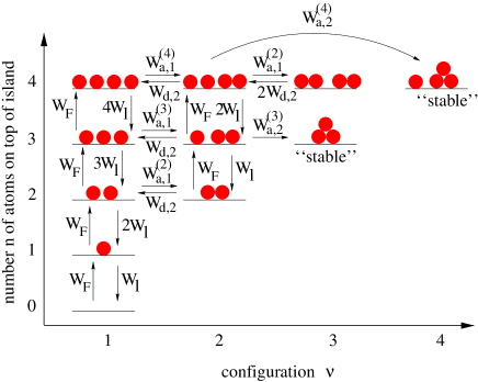
FIG. 12.: Various states and the corresponding transition rates (see eq. (V A)) involved in the second layer nucleation for a critical nucleus of size $i=2$.

introduced below, etc.); they are considered to be independent of $D$, $\alpha$ and $R$. In principle one should also take into account the possibility that a subcluster composed of more than one atom can dissociate from an unstable cluster. In fact, it has been argued that such cluster dissociations are sometimes more likely to occur than the dissociation of single atoms, as e.g. for dimer dissociation from a tetramer on a (100) surface by a kind of “shearing mode”.[51] For simplicity we will take into account only the dissociation of single atoms here, although conceptually the inclusion of cluster dissociation processes into the general treatment poses no difficulty. Also, we do not consider the influence of cluster mobilities. If one would allow for a small jump rate $D_{j}/a^{2}$ of a cluster of size $j\!\geq\!2$, the relative diffusion of a $j$ cluster and a single atom would be larger by a factor $1\!+\!D_{j}/D$ and accordingly we had to multiply $W_{{\rm a},j}^{(n)}$ in eq. (56) by this factor for $j\!\geq\!2$.

The method is best introduced by an example. To this end consider Fig. 12 that illustrates the situation for a critical nucleus of size $i\!=\!2$. Various states of the island are shown, which are distinguished according to the total number $n$ of atoms on top of the island, and the possible configurations that can be assumed for a given $n$. Between the states the possible transitions are marked by arrows that are labeled by the corresponding rates. Note that the loss from a state with $n$ single atoms is $n$ times larger than the loss from the state with one atom. It is clear that Fig. 12 shows only a small part of the possible states and in principle can be extended by including larger numbers $n$. However, as will be pointed out below, these states with larger $n$ do not contribute much to the onset of second layer nucleation. Moreover, we have not included states containing stable clusters of size $j\!>\!i\!+\!1$ and transitions between different states containing a stable nucleus of size $i\!+\!1$. These are irrelevant for the fraction $f_{0}(t)$ of covered islands at time $t$.

We denote by $p_{n,\nu}$ the probability for the island to be in state $(n,\nu)$, where $n$ refers to the number of atoms on top of the island and $\nu$ to a specific configuration for a given $n$. A complete description of the stochastic process amounts to specifying the set $\{p_{n,\nu}(t)\}$ of state probabilities at all times $t$. The time evolution of the $\{p_{n,\nu}(t)\}$ is described by the master equation

$$\frac{dp_{n,\nu}}{dt} = \sum_{n^{\prime},\nu^{\prime}}\bigl{[}W(n^{\prime},\nu^{\prime}\!\to\!n,\nu)\,p_{n^{\prime},\nu^{\prime}}$$ (59)

$$\phantom{\sum_{n^{\prime},\nu^{\prime}}}-W(n,\nu\!\to\!n^{\prime},\nu^{\prime})\,p_{n,\nu}\bigr{]}\,,$$

where for the rates $W(n,\nu\!\to\!n^{\prime},\nu^{\prime})$ the appropriate expressions from eq. (V A) have to be substituted (see Fig. 12). Note that transitions are possible only between a limited number of states. In the situation considered here, where only single atoms can leave the island, we have $W(n,\nu\to n^{\prime},\nu^{\prime})\!=\!0$ for $|n-n^{\prime}|\!\geq\!2$.

To treat the problem of second layer nucleation under generic growth conditions one has to solve the set of eqs. (59) for $R\!=\!R(t)$ with $R(t)$ from eq. (18) subject to the initial condition $p_{n,\nu}\!=\!\delta_{n,0}$. To this end it is convenient to solve (59) using $R$ as the independent variable. The integration of the differential equations (59) using standard solvers takes very little CPU time on ordinary workstations, so that results for $f_{0}(t)$ and $R_{c}(\alpha)$ can be obtained almost immediately. Numerical results are discussed in the following.

B Negligible Lifetimes of Unstable Clusters

In this subsection we consider the case $\Delta E_{j}^{\scriptscriptstyle\rm dis}\!=\!0$ that was treated extensively in Sec. IV. The fraction $f_{0}(t)$ of covered islands within our more general framework is given by

$$f_{0}(t)=\sum_{n=i\!+\!1}^{\infty}p_{n,\nu_{n}}(t)\,,$$ (60)

where $\nu_{n}$ is the configuration containing a stable nucleus for a given $n$ (for example, $\nu_{3}\!=\!3$ and $\nu_{4}\!=\!4$ in Fig. 12). In practice, states corresponding to large $n$ contribute a negligible amount up to times $t_{c}$, so that one needs to consider a finite maximum number of atoms $n_{\star}$ only ($n_{\star}\!=\!4$ in Fig. 12 turned out to be sufficient).

Figure 13a shows $f_{0}(t)$ and the probabilities $p_{n,\nu}(t)$ (labeled according to Fig. 12) as a function of the coverage $Fa^{2}t$ for $\alpha\!=\!10^{-4}$, and $\Gamma\!=\!10^{6}$. Also shown is the mean total number

$$N(t)\equiv\sum_{n=1}^{n_{\star}}\sum_{\nu\neq\nu_{n}}p_{n,\nu}(t)\,n$$ (61)

of atoms that are not in states possessing a stable nucleus. In accordance with the predictions of the simplified stochastic description, this number is less than one

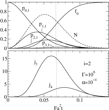
FIG. 13.: Time development of the fraction of covered islands $f_{0}(t)$, the mean number of atoms $N(t)$ in states containing no stable nucleus, the occupation probabilities $p_{n,1}$, and the currents $j_{3}$ and $j_{4}$ (see eq. 62) for $i\!=\!2$, $\alpha=10^{-4}$ and $\Gamma=10^{6}$. The maximum number of atoms is $n_{\star}\!=\!4$ corresponding to the digram shown in Fig. 12. The vertical dotted line marks the coverage $Fa^{2}t_{c}$ at the critical time $t_{c}$.

up to time $t_{c}$. Accordingly, the pathway followed by the system to form a stable nucleus is dominated by fluctuations as discussed in Sec. IV. The important role of the fluctuations can even more clearly be recognized by looking at the state probabilities $p_{n,\nu}$, $\nu\!\neq\!\nu_{n}$, and the currents

$$j_{3}(t)\equiv W_{{\rm a},2}^{(3)}\,p_{3,2}(t)\,,\hskip 14.22636ptj_{4}(t)\equiv W_{{\rm a},2}^{(4)}\,p_{4,2}(t)$$ (62)

into the states containing a stable nucleus. As can be seen from Fig. 13a, only the probabilities $p_{n,1}(t)$ are significant, while the other state probabilities $p_{n,2}(t)$ and $p_{4,3}(t)$ cannot be discerned on the scale used in the figure. On the other hand, we find that the current $j_{3}(t)$ from the state $(n\!=\!3,\nu\!=\!2)$ (which has a very small probability $p_{3,2}(t)$) contributes most to the growth of $f_{0}(t)$, see Fig. 13b. The fact that $j_{4}(t)$ gives only a subdominant contribution to second layer nucleation, indicates that the incorporation of states with $n\!>\!5$ will not significantly change the behavior of $f_{0}(t)$.

The results for $f_{0}(t)$ compare well with the data obtained from kinetic Monte Carlo simulations, the quality of agreement between theory and simulation being as good as in Fig. 4. The values of the optimal prefactors $\kappa_{\rm a,j}^{(n)}$ and $\kappa_{\rm d,2}$ are given in ref. [52]. To exemplify the good agreement between theory and simulations, we have re-plotted in Fig. 14 the critical radius $R_{c}$ as a function of $\alpha$ for various $\Gamma$ for $i\!=\!1,2$ from Figs. 8,10. The solid lines referring to the numerical results give an excellent fit to the Monte Carlo data. For $i\!=\!1$, only the states with $n\!\leq\!2$ in Fig. 12 had to be included to achieve this almost perfect agreement.

FIG. 14.: Comparison of critical island sizes $R_{c}$ obtained from the rate-equation approach (solid lines) with Monte Carlo data for critical nuclei $i=1,2$ and different values of $\Gamma$ (same symbols as in Figs. 8,10).

For $i\!>\!2$ we expect that a very large number $n_{\star}$ has to be chosen in order to obtain a correct description of second layer nucleation within the rate equation approach. Diagrams corresponding to that shown in Fig. 12 then become very complicated and not easily tractable from the practical point of view. It is thus helpful to introduce

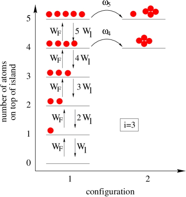
FIG. 15.: States and corresponding transition rates (see eqs. (V A,32)) involved in the second layer nucleation for a critical nucleus of size $i\!=\!3$ when the lifetimes of unstable clusters are neglected. Only states corresponding to $n\!\leq\!5$ atoms on top of the island are shown.

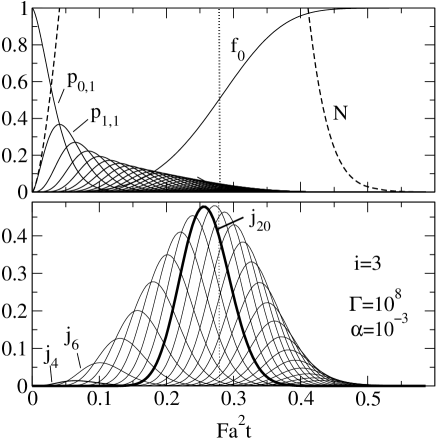
FIG. 16.: Time development of the fraction of covered islands $f_{0}(t)$, the mean number of atoms $N(t)$ in states containing no stable nucleus, the occupation probabilities $p_{n,1}$, and the currents $j_{n}(t)=\omega_{n}p_{n,1}$, $n\!\geq\!i\!+\!1$ for $i\!=\!3$, $\alpha=10^{-3}$ and $\Gamma=10^{8}$. The maximum number of atoms included in a diagram of the type shown in Fig. 15 is $n_{\star}\!=\!50$. The vertical dotted line marks the coverage $Fa^{2}t_{c}$ at the critical time $t_{c}$. At $t_{c}$ we find $N(t_{c})\!\cong\!10$.

the “renormalized” encounter rates $\omega_{n}$ defined in eq. (32) and to consider simplified diagrams as shown in Fig. 15 for $i\!=\!3$. For a given number $n\!\geq\!i\!+\!1$ of atoms on top of the island we have only included two states $\nu\!=\!1,2$: One of these refers to a state where all $n$ atoms are separated ($\nu\!=\!1$), and the other one to a state, where exactly $i\!+\!1$ atoms form a stable nucleus, while the remaining $n\!-\!(i\!+\!1)$ atoms are not bound to other atoms in the same layer $(\nu\!=\!2)$.

Plots of $f_{0}(t)$, $p_{n,1}(t)$, $N(t)$, and $j_{n}(t)\!\equiv\!p_{n,1}(t)\omega_{n}(R(t))$ for $i\!=\!3$ analogous to Fig. 13 are shown in Fig. 16. As expected from the discussion in Sec. IV, we now had to take into account states with $n$ up to $n_{\star}\!=\!50\!\gg\!i(i+1)/2\!=\!6$ before reaching the limit, where $f_{0}(t)$ as calculated from eq. (60) did not change much by incorporation of states with larger $n$. Near $t_{c}$, $N(t)$ is significantly larger than $i\!+\!1\!=\!4$ (at $t_{c}$ we find $N(t_{c})\cong 10$), and the dominant currents $j_{n}(t)$ initiating second layer nucleation are those for $n\!=\!15-20\!\gg\!4$, see Fig. 16.

In order to see how the preferred paths for second layer nucleation change with the step crossing probability $\alpha$, we define the integrated current $j_{n}(t)$ up to $t_{c}$ by

$$J_{n}\!\equiv\!\int_{0}^{t_{c}}dt\,j_{n}(t)\!=\!\int_{0}^{t_{c}}dt\,p_{n,1}(t)\omega_{n}(R(t))\,,\hskip 2.84544ptn\geq i\!+\!1\,.$$ (63)

This quantity equals the fraction of covered islands at time $t_{c}$ for which the stable nucleus originates from a state possessing exactly $n$ adatoms. Figure 17 shows $J_{n}$ as a function of $n$ for fixed $\Gamma=10^{8}$ and various $\alpha$. We

FIG. 17.: Integrated nucleation currents up to time $t_{c}$ as a function of the number of particles $n$ in the state from which the nucleation event took place ($i\!=\!3$).

see that for all $\alpha$ states with $n\!\gg\!4$ dominate the onset of the nucleation. The number of particles $n_{\rm peak}$ in the state where $J_{n}$ has a maximum strongly increases with increasing $\alpha$. For $\alpha\!=\!10^{-3}$, the second layer nucleation is typically initiated by $n_{\rm peak}\!\simeq\!18$ adatoms on top of the island.

C Influence of Metastable Clusters

The general procedure outlined in Sec. V A allows us also to describe situations, where the binding energies of unstable clusters of size $j\!\leq\!i$ are not small compared to $k_{\rm B}T$. To demonstrate this we again consider the case $i\!=\!2$ and the corresponding diagram in Fig. 12. The dimer in the intermediate states possessing no stable nucleus is now considered to be metastable, and we introduce the parameter

$$\beta\equiv\exp(-\Delta E_{j}^{\scriptscriptstyle\rm dis}/k_{\rm B}T)$$ (64)

as “dissociation probability” (analogous to the step edge crossing probability $\alpha=\exp(-\Delta E_{\rm S}/k_{\rm B}T)$). For $\beta=1$ we recover the non-interacting particle model. From the outset it is clear that second layer nucleation will proceed faster for smaller $\beta$, since the state probabilities $p_{3,2}(t)$ and $p_{4,2}(t)$ in Fig. 12 and accordingly the currents $j_{3}(t)$ and $j_{4}(t)$ defined in eq. 62 will become strongly enhanced.

Figure 18 shows $R_{c}$ as a function of $\alpha$ for fixed $\Gamma\!=\!10^{8}$ and various $\beta$ obtained from Monte Carlo simulations (open symbols). As expected, the critical radius decreases with decreasing $\beta$. In fact, for $\beta\!=\!10^{-6}$ one can regard the dimer as effectively being stable on the relevant time scale $t_{c}$, so that the changes with $\beta$ correspond to a continuous transition from $i\!=\!2$ ($\beta\!=\!1$) to $i\!=\!1$ ($\beta\!=\!10^{-6}$). The comparison with the numerical solution of eqs. 59 (solid lines) yields very good agreement. To achieve this agreement, we used the same set of prefactors $\kappa_{\rm a,j}^{(n)}$, $\kappa_{\rm d,2}$ as in Fig. 14.[52] This highlights the power of the rate equation approach to treat second layer nucleation in general situations.

FIG. 18.: Comparison of critical island sizes $R_{c}$ obtained from the rate-equation approach with results from kinetic Monte Carlo simulations of the one-island model for $i\!=\!2$. Dimers are metastable and dissociate with a rate $\beta D/a^{2}$ (see eq. (64)).

VI Summary and Discussion

In summary, we have presented a detailed theoretical investigation of the nucleation on top of islands in epitaxial growth. In the non-interacting particle model, where the lifetimes of unstable clusters can be neglected, it was possible to tackle the problem within a simplified stochastic description based on scaling arguments. An important result for the non-interacting case is that the nucleation for critical nuclei of size $i\!\leq\!2$ is dominated by fluctuations, while for larger critical nuclei it can be treated in a mean-field type manner. The second layer nucleation rate for both cases was derived in compact form (see eqs. (42,40)). When metastable clusters can form with appreciable lifetimes, the simplified description can in principle be extended (see Sec. IV E), but becomes of limited value due to the fact that many elementary processes get mutually coupled both sequentially and in parallel. In such situations it is better to employ the more general framework outlined in Sec. V that is based on our derivation for the transition rates of the elementary processes. Results obtained from both theoretical approaches were shown to agree with Monte Carlo data.

Throughout the paper, we have used the generic growth law (18) for the mean island radius, but it is straightforward to treat other growth laws also (as e.g. an exponential behavior), which may be realized by special preparation techniques.[11] Neither the general expressions (40,42) for the second layer nucleation rates in simple situations nor the master equation (59) depend on the specific form of the growth law (the expressions for $\bar{n}$, $p_{n}$, etc. in the quasi-stationary case however get modified, see the discussion in Sec. IV A). Moreover, it is straightforward to rewrite all formulae for the case of heteroepitaxy by replacing the jump rate $D/a^{2}$ of adatoms on top of the islands by a modified jump rate $D^{\prime}/a^{2}$.

The theoretical understanding of second layer nucleation is not only of basic importance but has numerous applications. One of these is the determination of the effective step edge barrier $\Delta E_{\rm S}$ for systems, where the more direct and simpler method via the measurement of adatom lifetimes by field ion microscopy[53] cannot be applied. As pointed out in ref. [16], the breakdown of the TDT approach in the fluctuation-dominated situation calls for a reexamination of some experimental data for estimating $\Delta E_{\rm S}$. In fact, such reexamination has been carried out recently by Krug et al.[17] with notable results: By reanalyzing the fraction of covered islands $f(t)$ measured for Ag/Ag(111)[11] they corrected the previously reported estimate $\Delta E_{s}\!\approx\!0.12{\rm eV}$ to $\Delta E_{s}\!\approx\!0.32{\rm eV}$ (they also reported another estimate yielding $\Delta E_{s}\!\approx\!0.20{\rm eV}$ based on a modified data analysis, see the comment in ref. [54]). Krug et al. moreover studied the influence of step decoration by CO molecules[55] on $R_{c}$ (and hence $\Delta E_{\rm S}$) for Pt/Pt(111). They found a strong increase of $\Delta E_{\rm S}$ with CO partial pressures, when analyzing the data corresponding to regime II (for $i\!=\!1$) of the fluctuation-dominated situation. Hence contamination by CO is expected to favor multilayer growth.

On the other hand, surfactants may promote smooth layer-by-layer growth. For example, the presence of only small amounts of Sb for growth of Ag on Ag(111) were shown to convert rough multilayer to layer-by-layer growth.[56, 57] It was suggested[56] that Sb reduces $\Delta E_{\rm S}$, but, since it was observed that Sb increases the island density in the first layer,[56, 7] it is also possible that the induced layer-by-layer growth results from a decrease of the mean island distance. Even in the absence of surfactants, a change of the effective step edge barrier may go along with a shape transition of the islands with varying temperature (see refs. [58, 59, 60, 7] and the comment in ref. [23]), and this can induce changes in the film morphology as well. With respect to the transition from the fluctuation-dominated to the mean-field type situation with varying $i$ predicted in this work, it would also be interesting to conduct proper experiments for metal epitaxy on (100) surfaces, where a change from $i\!=\!1$ to $i\!=\!3$ is often observed with increasing temperature.

A further application pertaining to the design of self-organized nanostructures is the possibility to create pyramidal mounds on a substrate, which are called “wedding cakes”.[61, 62, 63] As suggested by Michely et al.,[64] the size $L_{\rm top}$ of the top terrace of the pyramid should be roughly given by $\Omega(L_{\rm top})\approx F$, where $\Omega$ is the second layer nucleation rate. Recently, an expression for the distribution of $L_{\rm top}$ has been suggested within a self-consistent analysis of a model for the dynamics of the top terrace.[17] In recent developments of nanostructure formation also larger clusters of atoms are considered as basic building blocks in epitaxial growth. The underlying processes seem to be very similar to the case of deposition of single atoms or simple molecules (for a recent review, see Ref. [65]), so that it could well be that also for cluster deposition an effective step edge barrier has a decisive influence on the film topography.

In light of the basic importance and the manifold applications, there is certainly need for further improvement of our understanding of second layer nucleation. Topics worthy of further study are in particular the influence of strain effects and longer-range interactions between the adatoms. The latter may be attributed to direct forces (e.g. induced dipole-dipole forces in the case of magnetic adsorbates), or they can be mediated by perturbations of the electron structure of the substrate. By extending the approach presented in this work, these issues may be tackled in the near future.

A

We want to calculate the characteristic rate $\omega_{n}(R)$ for an encounter of $i\!+\!1$ atoms, if initially $n\!\geq\!i\!+\!1$ atoms are randomly placed on top of an island with radius $R$ and infinite step edge barrier ($\alpha\!=\!0$). For this purpose let us consider the encounter as a sequential process as depicted in Fig. 19 (for $i\!=\!3$ and $n\!=\!5$): First a dimer forms, then one of the remaining atoms attaches to the dimer and a trimer is created, and so on until a stable cluster composed of $i\!+\!1$ atoms has been formed. Denoting the rate for the formation of the dimer by $w_{1}$, and the rate for the attachment of an atom to an already existing cluster composed of $k$ atoms (“$k$-cluster”) by $w_{k}$, we may write

$$w_{1}=\frac{n(n\!-\!1)}{2}\,\frac{2D}{a^{2}}\,\frac{b_{1}a^{2}}{\pi R^{2}}\,,$$ (A2)

$$w_{k}=(n\!-\!k)\,\frac{D}{a^{2}}\,\frac{b_{k}a^{2}}{\pi R^{2}}\,,\hskip 17.07182pt2\!\leq\!k\!\leq\!i\,.$$ (A3)

The factors $b_{k}$ can be viewed as the effective number of perimeter sites of a $k$-cluster. Similarly, we may writefor the rate of dissociation $v_{k}$ of a single atom from a $k$-cluster (in the case of negligible binding energies of unstable clusters)

$$v_{k}=d_{k}\,\frac{D}{a^{2}}\,,\hskip 17.07182ptk\!\geq\!2\,,$$ (A4)

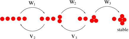
FIG. 19.: Illustration of the encounter of 4 atoms out of $n\!=\!5$ adatoms. The 4 connected atoms are supposed to form a stable cluster ($i\!=\!3$). First a dimer forms with a rate $w_{1}$ then a trimer with a rate $w_{2}$, and finally the stable quadrumer with a rate $w_{3}$. The sequential process only leads to the formation of a stable cluster, if neither the dimer dissociates with the rate $v_{2}$ nor the trimer dissociates with the rate $v_{3}$.

where again $d_{k}$ has the meaning of an effective number of perimeter sites. (In principle one may also take into account the possibility that a subcluster composed of more than one atom can dissociate from an unstable cluster and other states with various intermediate unstable clusters of size $2\!\leq\!k\!\leq\!i$.)

The idea now is to renormalize the process depicted in Fig.19 by replacing it by an effective transition rate $w_{\rm eff}$ between the initial state composed of $n$ isolated atoms and the final state containing the stable cluster. Clearly, such a replacement is only approximately valid. After the replacement, the encounter rate $\omega_{n}(R)$ in eq. (32) can be identified with $w_{\rm eff}$. In order to derive $w_{\rm eff}$, we consider a stationary situation, where the probability $p_{1}$ of the initial state is kept fixed and a constant current $J$ flows between neighboring states containing a $k$- and $k\!+\!1$-cluster. We thus write

$$J=w_{k}p_{k}-v_{k+1}p_{k+1}\,,\hskip 14.22636pt1\!\leq\!k\!\leq\!i\!-\!1\,,$$ (A5)

where $p_{k}$ denotes the probability of the state containing a $k$-cluster. The set of equations (A5) can be readily solved for $p_{i}$ yielding

$$J=w_{i}p_{i}=w_{1}p_{1}\prod_{k=2}^{i}\frac{w_{k}}{v_{k}}-J\sum_{k=2}^{i}\prod_{j=k}^{i}\frac{w_{j}}{v_{j}}\,.$$ (A6)

On the other hand we have

$$J=w_{\rm eff}p_{1}\,.$$ (A7)

Eliminating $J$ from eqs. (A6,A7), we obtain

$$w_{\rm eff}=\frac{w_{1}\prod_{k=2}^{i}w_{k}/v_{k}}{1+\sum_{k=2}^{i}\prod_{j=k}^{i}w_{j}/v_{j}}\,.$$ (A8)

For large radii $R\!\gg\!a$, it holds $w_{j}/v_{j}\!\ll\!1$ so that we can neglect the sum over $k$ in the denominator on the right hand side of (A8). Hence we find

$$\omega_{n}(R)\simeq w_{\rm eff}\simeq\kappa_{\rm e}\left[\prod_{k=0}^{i}(n\!-\!k)\right]\,\frac{D}{a^{2}}\,\left(\frac{a^{2}}{\pi R^{2}}\right)^{i}\,,$$ (A9)

where $\kappa_{\rm e}\!=\!b_{1}\prod_{k=2}^{i}b_{k}/d_{k}$.

B

The solution of the diffusion problem[34]

$$\frac{\partial\rho}{\partial t}=D\,\Delta\rho\,,$$ (B2)

$$\frac{\partial\rho}{\partial r}\Bigl{|}_{r=0}=0\,,\hskip 11.38092pt\left[\frac{\partial\rho}{\partial r}+\frac{\alpha}{a}\rho\right]_{r=R}=0$$ (B3)

with the initial condition $\rho({\bf r},t\!=\!0)=1/(\pi R^{2})$ has been derived by Harris:[47]

$$\rho({\bf r},t)=\sum_{k=1}^{\infty}\frac{c_{k}\lambda_{k}^{2}}{2\pi R^{2}{\textstyle\frac{\textstyle\alpha R}{\textstyle a}}}\,\frac{J_{0}({\textstyle\frac{\textstyle\lambda_{k}r}{\textstyle R}})}{J_{0}(\lambda_{k})}\,\exp\Bigl{(}-\lambda_{k}^{2}\frac{D}{R^{2}}t\Bigr{)}\,.$$ (B4)

Here $J_{\nu}(.)$ is the Bessel function of $\nu$th order, $c_{k}\!\equiv\!4(\alpha R/a)^{2}/(\lambda_{k}^{2}[\lambda_{k}^{2}\!+\!(\alpha R/a)^{2}])$ and $\lambda_{k}$ is the $k$th root ($\lambda_{1}\!<\!\lambda_{2}\!<\!\ldots$) of

$$\Bigl{(}\frac{\alpha R}{a}\Bigr{)}J_{0}(\lambda)=\lambda J_{1}(\lambda)\,.$$ (B5)

The solution (B4,B5) describes the probability density for a single diffusing atom that at time $t\!=\!0$ is randomly deposited on top of a circular island with a partially reflecting boundary. The probability that the atom has not escaped from the island up to time $\tau$ is $\Psi(\tau)\!=\!2\pi\int_{0}^{R}dr\,r\,\rho({\bf r},t)$, which yields[47]

$$\Psi(\tau)=\sum_{k=1}^{\infty}c_{k}\exp\Bigl{(}-\lambda_{k}^{2}\frac{D}{R^{2}}\tau\Bigr{)}$$ (B6)

Note that, since $\Psi(0)\!=\!1$, it must hold $\sum_{k=1}^{\infty}c_{k}\!=\!1$.

The probability that none of $n$ independent atoms has escaped from the island up to time $\tau$ is $\Psi(\tau)^{n}$. Accordingly, the probability $\phi(\tau)d\tau$ that the first atom leaves the island in the time interval $[\tau,\tau\!+\!d\tau]$ is

$$\phi(\tau) = -\frac{d\Psi(\tau)^{n}}{d\tau}=-n\Psi(\tau)^{n\!-\!1}\,\frac{d\Psi(\tau)}{d\tau}$$ (B7)

$$= n\frac{D}{R^{2}}\sum_{j_{1},\ldots,j_{n}=1}^{\infty}c_{j_{1}}{\scriptstyle\ldots}c_{j_{n}}\,\times$$ (B9)

$$\hskip 51.21504pt\times\,\lambda_{j_{1}}^{2}\exp\Bigl{[}-(\lambda_{j_{1}}^{2}\!+\!{\scriptstyle\ldots}\!+\!\lambda_{j_{n}}^{2})\frac{D}{R^{2}}\,\tau\Bigr{]}\,,$$

from which for the average time $\tau_{n}(R)\!\equiv\!\int_{0}^{\infty}d\tau\phi(\tau)\tau$ follows:

$$\tau_{n}(R)=n\frac{R^{2}}{D}\sum_{j_{1},\ldots,j_{n}=1}^{\infty}c_{j_{1}}{\scriptstyle\ldots}c_{j_{n}}\frac{\lambda_{j_{1}}^{2}}{(\lambda_{j_{1}}^{2}\!+\!{\scriptstyle\ldots}\!+\!\lambda_{j_{n}}^{2})^{2}}\,.$$ (B10)

It is easy to show that $j_{1,k}\!<\!\lambda_{k}\!<\!j_{0,k}$, where $j_{\nu,k}$ is the $k$th zero of $J_{\nu}(.)$. Since $j_{\nu,k}\!\sim\!(k\!+\!\nu/2\!-\!1/4)\pi$ for $k\!\gg\!\nu$, the terms in the series of (B10) rapidly decrease with increasing $j_{k}$, $k\!=\!1,\ldots,n$ (note that $c_{j}$ depends on $\lambda_{j}$). The leading term can be obtained by setting $c_{j}=\delta_{j,1}$ in eq. (B6), which amounts to a Poisson approximation of the escape process, $\Psi(\tau)\simeq\exp(-\lambda_{1}D\tau/R^{2})$. Within this approximation we obtain

$$\tau_{n}(R)=\frac{1}{n}\frac{R^{2}}{D}\frac{1}{\lambda_{1}^{2}}\,,$$ (B11)

where $\lambda_{1}$ follows from eq. (B5). In the limit of small $\alpha R/a\ll 1$ one finds $\lambda_{1}^{2}\simeq 2\alpha R/a$, while in the limit of large $\alpha R/a\gg 1$, $\lambda_{1}^{2}\simeq j_{0,1}^{2}$. Combining these two limits yields the interpolation formula

$$\tau_{n}(R)\simeq\frac{1}{n}\,\frac{R^{2}}{D}\,\left(\kappa_{1}\frac{a}{\alpha R}+\kappa_{2}\right)$$ (B12)

with $\kappa_{1}\!=\!1/2$ and $\kappa_{2}\!=\!1/j_{0,1}^{2}\!\cong\!0.173$.

Knowing $\tau_{n}(R)$ we can set up the master equation for the probabilities $p_{n}(t)$ to find exactly $n$ atoms on top of the island at time $t$ in the presence of an incoming flux $F$, see eq. (35). Introducing the generating function $Q(z,t)\!\equiv\!\sum_{n=0}^{\infty}p_{n}(t)z^{n}$ we obtain from eq. (35)

$$\frac{\partial Q}{\partial t}\!=\!(z\!-\!1)\left[\pi FR^{2}Q-\frac{1}{\tau_{1}(R)}\frac{\partial Q}{\partial z}\right]\,,$$ (B13)

where $R\!=\!R(t)$ from eq. (18). Transforming variables from $t$ to $R$ and defining $\tilde{Q}(z,R)$ by $\tilde{Q}(z,R\!=\!R(t))\!\equiv\!Q(z,t)$, eq. (B13) gives ($a\equiv 1$ here)

$$\frac{\partial\tilde{Q}}{\partial R}+\frac{\varphi\tilde{\alpha}}{1\!+\!\tilde{\alpha}R}(z\!-\!1)\frac{\partial\tilde{Q}}{\partial z}=\frac{2\pi}{A^{2}\Gamma^{i/(i\!+\!2)}}R^{3}(z\!-\!1)\tilde{Q}\,,$$ (B14)

where $\tilde{\alpha}\!=\!\kappa_{2}\alpha/\kappa_{1}$ and $\varphi\!=\!2A^{-2}\Gamma^{2/(i\!+\!2)}/\kappa_{2}$ Equation (B14) is a semi-linear partial differential equation of first order that can be solved by the method of characteristics. For the initial condition $\tilde{Q}(z,R=0)\!=\!1$ we obtain

$$\tilde{Q}(z,R)=\exp\left[-(1-z)\bar{n}(R)\right]\,,$$ (B15)

which for $p_{n}(R)\!=\!p_{n}(R(t))\!=\![\partial_{z}^{n}\tilde{Q}(z,R)/n!]_{z=0}$ yields the Poisson distribution (36) with

$$\bar{n}(R) = \frac{2\pi}{A^{2}\Gamma^{\scriptstyle\frac{i}{i\!+\!2}}}(1\!+\!\tilde{\alpha}R)^{-\varphi}\int_{0}^{R}dx\,x^{3}\,(1\!+\!\tilde{\alpha}x)^{\varphi}$$ (B16)

$$= \frac{2\pi}{A^{2}\Gamma^{\scriptstyle\frac{i}{i\!+\!2}}\tilde{\alpha}^{4}}(1\!+\!\tilde{\alpha}R)^{-\varphi}$$ (B19)

$$\hskip 5.69046pt\times\Biggl{[}\frac{(1\!+\!\tilde{\alpha}R)^{\varphi\!+\!4}-1}{\varphi\!+\!4}-3\frac{(1\!+\!\tilde{\alpha}R)^{\varphi\!+\!3}-1}{\varphi\!+\!3}$$

$$\hskip 5.69046pt\phantom{\times\Biggl{[}}{}+3\frac{(1\!+\!\tilde{\alpha}R)^{\varphi\!+\!2}-1}{\varphi\!+\!2}-\frac{(1\!+\!\tilde{\alpha}R)^{\varphi\!+\!1}-1}{\varphi\!+\!1}\Biggr{]}\,.$$

In the quasi-stationary case ($\partial_{t}Q\!=\!0$ in eq. (B13)) one obtains

FIG. 20.: Sketch of the island geometry in the neighborhood of a boundary site $\mathbf{l}$, from which two jumps in the directions $\mbox{\boldmath$\delta$}_{1}$ and $\mbox{\boldmath$\delta$}_{2}$ lead to an escape from the island over the step edge barrier.

$$\bar{n}^{\scriptscriptstyle\rm st}(R)=\pi FR^{2}\tau_{1}(R)=\pi\frac{FR^{4}}{D}\left(\kappa_{1}\frac{a}{\alpha R}+\kappa_{2}\right)\,,$$ (B20)

to which (B19) simplifies for $\varphi\tilde{\alpha}R\!\ll\!1$ (see the discussion right after eq. (37)).

Alternatively, we can determine $\bar{n}^{\scriptscriptstyle\rm st}(R)$ by integrating $\rho_{1}^{\scriptscriptstyle\rm st}(r)$ over the island area, which yields

$$\bar{n}^{\scriptscriptstyle\rm st}(R)\!=\!2\pi\int_{0}^{R}dr\,r\,\rho_{1}^{\scriptscriptstyle\rm st}(r)\!=\!\pi\frac{FR^{4}}{D}\left(\frac{1}{2}\frac{a}{\alpha R}+\frac{1}{8}\right)\,.$$ (B21)

Hence we can improve the Poisson approximation by renormalizing the bare coefficient $\kappa_{2}\!=\!1/j_{0,1}^{2}\!\simeq\!0.173$ to $\kappa_{2}\!=\!1/8$ (note that $\kappa_{1}\!=\!1/2$ does not change).

Finally, in order to obtain the constants $\kappa_{1}$ and $\kappa_{2}$ in eq. (33), one has to take into account the “lattice corrections”. Let us denote by ${\mathbf{l}}$ the position of a lattice site and by $\mbox{\boldmath$\delta$}_{j}$ the nearest-neighbor bond vectors, i.e. for a triangular lattice $\mbox{\boldmath$\delta$}_{j}\!=\!(\cos[2\pi j/6],\sin[2\pi j/6])a$, $j\!=\!0,\ldots,5$. The master equation describing the diffusion of a single adatoms on the island reads

$$\frac{\partial w({\mathbf{l}},t)}{\partial t}=\frac{D}{6a^{2}}\sum_{j=0}^{5}\left[w({\mathbf{l}}+\mbox{\boldmath$\delta$}_{j},t)-w({\mathbf{l}},t)\right]\,,$$ (B22)

where $w({\bf l},t)$ is the probability to find the atom at lattice site ${\bf l}$. Equation (B22) is valid as long as ${\mathbf{l}}$ is not a boundary site. In the continuum limit we can write $\sum_{j=0}^{5}[w({\mathbf{l}}+\mbox{\boldmath$\delta$}_{j},t)-w({\mathbf{l}},t)]\!=\!(1/2)\sum_{j=0}^{5}(\mbox{\boldmath$\delta$}_{j}\cdot\mbox{\boldmath$\nabla$})^{2}w({\mathbf{l}},t)+{\mathcal{O}}(a^{4})$, which yields eq. (B2) when $D$ is replaced by $D_{\rm cont}=D/4$ (see also the remark in ref. [34]). As a consequence, one has to substitute $D$ by $D_{\rm cont}$ in all continuum equations, in particular in eq. (B21), which means that in eq. (33) (referring to the lattice simulations) one should take $\kappa_{1}\!=\!4(1/2)\!=\!2$ and $\kappa_{2}\!=\!4(1/8)\!=\!1/2$.

The value of $\kappa_{1}$ is still not correct, since we have not taken into account the lattice correction to the parameter $\alpha$. To derive this correction we consider a lattice site ${\mathbf{l}}$ at the boundary. For example, one may encounter the situation sketched in Fig. 20, where $\mbox{\boldmath$\delta$}_{0}$ and $\mbox{\boldmath$\delta$}_{1}$ lead to sites outside the island (where $w({\mathbf{l}}+\mbox{\boldmath$\delta$}_{j},t)\!\equiv\!0$) and the remaining nearest neighbor sites ${\mathbf{l}}+\mbox{\boldmath$\delta$}_{j}$, $j\!=\!2,\ldots,5$ are on the island. The equation corresponding to (B22) then reads

$$\frac{\partial w({\mathbf{l}},t)}{\partial t} = \frac{\alpha D}{6a^{2}}\sum_{j=0}^{1}\left[w({\mathbf{l}}+\mbox{\boldmath$\delta$}_{j},t)-w({\mathbf{l}},t)\right]$$ (B24)

$${}+\frac{D}{6a^{2}}\sum_{j=2}^{5}\left[w({\mathbf{l}}+\mbox{\boldmath$\delta$}_{j},t)-w({\mathbf{l}},t)\right]$$

$$= -\frac{2\alpha D}{6a^{2}}w({\mathbf{l}},t)+\frac{D}{6a^{2}}\sum_{j=0}^{5}\left[w({\mathbf{l}}+\mbox{\boldmath$\delta$}_{j},t)-w({\mathbf{l}},t)\right]$$ (B26)

$${}-\frac{D}{6a^{2}}\sum_{j=0}^{1}\left[w({\mathbf{l}}+\mbox{\boldmath$\delta$}_{j},t)-w({\mathbf{l}},t)\right].$$

In a discretization of the second boundary condition in eq. (B3) on a triangular lattice one has to eliminate the outer boundary points ${\mathbf{l}}+\mbox{\boldmath$\delta$}_{0}$ and ${\mathbf{l}}+\mbox{\boldmath$\delta$}_{1}$ via the discretized version of the “bulk equation” (B3). This amounts to a cancellation of the term on the left hand side and the second term on the right hand side of (B26) in the continuum limit, and the replacement $\sum_{j=0}^{1}[w({\mathbf{l}}\!+\!\mbox{\boldmath$\delta$}_{j},t)\!-\!w({\mathbf{l}},t)]\!=\!\sum_{j=0}^{1}(\mbox{\boldmath$\delta$}_{j}\cdot\mbox{\boldmath$\nabla$})w({\mathbf{l}},t)+{\mathcal{O}}(a^{2})\!\to\!\sqrt{3}a\partial w/\partial r$. Hence eq. (B26) corresponds to the second boundary condition in eq. (B3), when $\alpha$ is replaced by $\alpha_{\rm cont}=2\alpha/\sqrt{3}$ in eq. (B3).

In general, $k$ nearest neighbor sites of a boundary site ${\mathbf{l}}$ can lie outside the island ($k\!=\!1,\ldots,4$). The weights how often such ${\mathbf{l}}$ occur and the way the normal direction is oriented with respect to the nearest neighbor bond vectors leading to the sites outside the island depend sensitively on the shape of the island edge. Hence, the factor $2/\sqrt{3}$ is only an estimate, which gives an impression on the influence of the lattice correction to the coefficient $\kappa_{1}$. Our comparison with the simulation results in Fig. 7 yields $\alpha_{\rm cont}\!\cong\!2\alpha$, i.e. $\kappa_{1}\!\cong\!4(1/2)^{2}\!=\!1$. We note that in general lattice corrections have always to be included in a continuum description after the effective Schwoebel barrier (for the lattice) has been calculated from the microscopic barriers (see the comment in ref. [23]).

REFERENCES

- [1] J. A. Venables, G. D. T. Spiller, and M. Hanbücken, Rep. Prog. Phys. 47, 399 (1984).
- [2] M. Volmer and A. Weber, Z. Phys. Chem. (Leipzig) 119, 277 (1926).
- [3] I. N. Stranski and L. Krastanov, Sitzungsber. Akad. Wiss. Wien 146, 797 (1938).
- [4] E. Bauer and J. H. v. d. Merwe, Phys. Rev. B 33, 3657 (1986).
- [5] H. Brune, Surf. Sci. Rep. 31, 121 (1998).
- [6] P. Politi, G. Grenet, A. Marty, A. Ponchet and J. Villain, Phys. Rep. 324, 271 (2000).
- [7] J. Tersoff, A. W. Denier van der Gon, and R. M. Tromp, Phys. Rev. Lett. 72, 266 (1994).
- [8] G. Ehrlich and F. G. Hudda, J. Chem. Phys. 44, 1039 (1966); R. L. Schwoebel, J. Appl. Phys. 40, 614 (1969).
- [9] Z. Zhang and M. G. Lagally, Phys. Rev. Lett. 72, 693 (1994); Z. Zhang and M. G. Lagally, Science 276, 377 (1997).
- [10] S. Das Sarma, P. Punyindu, and Z. Toroczkai, e-print cond/mat 9908013.
- [11] K. Bromann, H. Brune, H. Röder, and K. Kern, Phys. Rev. Lett. 75, 677 (1995).
- [12] J. A. Meyer, J. Vrijmoeth, H. A. van der Vegt, E. Vlieg, and R. J. Behm, Phys. Rev. B 51, R14790 (1995).
- [13] P. Šmilauer and S. Harris, Phys. Rev. B 51, R14798 (1995).
- [14] I. Markov, Phys. Rev. B 54, 17930 (1996).
- [15] K. R. Roos and M. C. Tringides, Surface Review and Letters 5, 833 (1998).
- [16] J. Rottler and P. Maass, Phys. Rev. Lett. 83, 3490 (1999)
- [17] J. Krug, P. Politi, and T. Michely, Phys. Rev. B, scheduled for issue on May 15, see also e-print cond/mat 9912410.
- [18] I. Elkinani and J. Villain, J. Phys. I France 4, 949 (1994).
- [19] S. Havlin and D. Ben Avraham, Adv. Phys. 36, 695 (1987).
- [20] A.-L. Barabási and H. E. Stanley, Fractal Concepts in Surface Growth (Cambridge University Press, 1995).
- [21] M. Plischke and Z. Rácz, Phys. Rev. Lett. 53, 415 (1984).
- [22] Ab initio calculation for microscopic step edge barriers have been performed e.g. by P. J. Feibelman, Phys. Rev. Lett. 81, 168 (1998).
- [23] For the calculation of the effective step edge barrier that determines the total escape rate from an island, one should average over the local escape rates associated with the set of microscopic barriers along the island edge. Accordingly, , where denotes an average over the (with an appropriate weighting by the probabilities of an adatom to be at the corresponding boundary sites). Note that for fractal island boundaries this averaging may result in an effective that depends on .
- [24] J. G. Amar and F. Family, Phys. Rev. B 54, 14742 (1996); J. G. Amar and F. Family, Thin Solid Films 272, 208 (1996).
- [25] For the definition of the Voronoi cell, see e.g. J. M. Ziman, Models of Disorder, (Cambridge University Press, 1979); In principle one should define the “dividing lines” in the Voronoi construction with respect to the island boundaries, which would lead to curved perimeters of capture areas.
- [26] The critical nucleus should be defined more precisely by referring to a particular atomic configuration. For simplicity we do not distinguish between the various possible configurations for a given island size.
- [27] H. Brune, G. S. Bales, J. Jacobsen, C. Boragno, and K. Kern, Phys. Rev. B 60, 5991 (1999).
- [28] S. L. Tang, P. F. Carcia, D. Coulman, and A. J. McGhie, Appl. Phys. Lett. 59, 2898 (1991).
- [29] M. C. Bartelt and J. W. Evans, Phys. Rev. B 46, 12675 (1992).
- [30] G. S. Bales and D. C. Chrzan, Phys. Rev. B 50, 6057 (1994).
- [31] J. G. Amar and F. Family, Phys. Rev. Lett. 74, 2066 (1994).
- [32] H. Röder, H. Brune, J. P. Bucher, and K. Kern, Surf. Sci. 298, 121 (1993); H. Brune, C. Romainczyk, H. Röder, and K. Kern, Nature 369, 469 (1994).
- [33] T. Michely, M. Hohage, M. Bott, and G. Comsa, Phys. Rev. Lett. 70, 3943 (1993).
- [34] To simplify notation, we do not distinguish between the diffusion coefficient in the continuum limit and the coefficient defining the jump rate of the adatoms on the substrate lattice. In two dimensions . In the case of heteroepitaxy, moreover, one has to replace by the jump rate on top of an island. Also, we do not introduce the edge crossing probability in the continuum limit, where the correction factor depends on both the lattice type and the shape of the island boundary. For a discussion of the lattice corrections, see Appendix B.
- [35] M. C. Bartelt and J. W. Evans, Surface Science 423, 189 (1999); M. C. Bartelt and J. W. Evans, Surf. Sci. Lett. 314, L829 (1994).
- [36] M. Bott, M. Hohage, M. Morgenstern, T. Michely, and G. Comsa, Phys. Rev. Lett. 76, 1304 (1996).
- [37] J. G. Amar, F. Family, and P.-M. Lam, Phys. Rev. B 50, 8781 (1994).
- [38] S. Liu, Z. Zhang, G. Comsa, and H. Metiu, Phys. Rev. Lett. 71, 2967 (1993).
- [39] M. C. Bartelt and J. W. Evans, Phys. Rev. Lett. 75 4250 (1995).
- [40] Writing for the in-layer hopping rate and for the hopping rate over the step edge, one should more generally take , if the attempt frequencies and are different.
- [41] C. Ratsch, A. Zangwill, P. Šmilauer, and D. D. Vvedensky, Phys. Rev. Lett. 72, 3194 (1994).
- [42] S.-C. Wang and G. Ehrlich, Phys. Rev. Lett. 67, 2509 (1991).
- [43] R. Stumpf and M. Scheffler, Phys. Rev. Lett. 72, 254 (1994).
- [44] J. Jacobsen, K. Jacobsen, P. Stoltze, and J. Nørskov, Phys. Rev. Lett. 74, 2295 (1995).
- [45] J. A. Stroscio and D. T. Pierce, Phys. Rev. B 49, 8522 (1994).
- [46] P. A. Mulheran and D. A. Robbie, Europhys. Lett. 49, 617 (2000).
- [47] S. Harris, Phys. Rev. B 52, 16793 (1995).
- [48] It is possible to include this spatial dependence of the diffusion profile into the stochastic description but the treatment then becomes comparable in complexity with a direct Monte Carlo simulation of the second layer nucleation process.
- [49] If one would deal with a physical situation not considered in this work, where the mobility of adatoms is irrelevant.
- [50] H. Kallabis, P. L. Krapivsky, and D. E. Wolf, Eur. Phys. J B 5, 801 (1998).
- [51] Z.-P. Shi, Z. Zhang, A. K. Swan, and J. F. Wendelken, Phys. Rev. Lett. 76, 4927 (1996).
- [52] For the various prefactors entering the transition rates displayed in Fig. 12 are , , , , , and . The relatively large factor may be understood as effectively taking into account the additional pathways resulting from states with . For we found to give an optimal fit for a reduced diagram, in which only the states with from Fig. 12 are taken into account .
- [53] K. Kyuno and G. Ehrlich, Phys. Rev. Lett. 81, 5592 (1998).
- [54] The attempt frequency for the jumps over the step edge (see the comment in ref. [40]), however, turned out to be unphysically large. When assuming the attempt frequency for in-layer jumps to be the same as , the experimental data could be fitted by allowing for a very slight decrease of with increasing temperature from for to for .
- [55] M. Kalff, G. Comsa, and Th. Michely, Phys. Rev. Lett. 81, 1255 (1998).
- [56] H. A. van der Vegt, H. M. van Pinxteren, M. Lohmeier, E. Vlieg, and J. M. C. Thornton, Phys. Rev. Lett. 68, 3335 (1992).
- [57] J. Vrijmoeth, H. A. van der Vegt, J. A. Meyer, E. Vlieg, and R. J. Behm, Phys. Rev. Lett. 72, 3843 (1994).
- [58] R. Kunkel, B. Poelsema, L. K. Verheij, and G. Comsa, Phys. Rev. Lett. 65, 7333 (1990).
- [59] M. Bott, T. Michely, and G. Comsa, Surf. Sci. 272, 161 (1992).
- [60] P. Šmilauer, M. R. Wilby, and D. D. Vvedensky, Phys. Rev. B 47, 4119 (1993).
- [61] H. J. Ernst, F. Fabre, R. Folkerts, and J. Lapujoulade, Phys. Rev. Lett. 72, 112 (1994).
- [62] M. Kalff, P. Šmilauer, G. Comsa and T. Michely, Surf. Sci. Lett., 426, L447 (1999).
- [63] R. Gerlach, Th. Maroutian, L. Douillard, and H.-J. Ernst, to be published.
- [64] T. Michely, M. Kalff, J. Krug, P. Politi, Physikalische Blätter 55, No. 11, 53 (1999).
- [65] P. Jensen, Rev. of Mod. Phys. 71, 1695 (1999).