Reaction Diffusion Models Describing a Two-lane Traffic Flow

M. Ebrahim Fouladvand

Department of Physics, Sharif University of Technology,
P.O.Box 11365-9161, Tehran, Iran
and

Institute for Studies in Theoretical Physics and Mathematics,
P.O.Box 19395-5531, Tehran, Iran

A uni-directional two-lane road is approximated by a set of two parallel closed one-dimensional chains. Two types of cars i.e. slow and fast ones are considered in the system. Based on the Nagel-Schreckenberg (Na-Sch) model of traffic flow [15], a set of reaction-diffusion processes are introduced to simulate the behaviour of the cars. Fast cars can pass the slow ones using the passing-lane. We write and solve the mean field rate equations for the density of slow and fast cars respectively. We also investigate the properties of the model through computer simulations and obtain the fundamental diagrams . A comparison between our results and $v_{max}=2$ version of Na-Sch model is made.

PACS number: 02.50.Ey , 05.70.Ln , 05.70.Fh , 82.20.Mj

Key words: two-lane road, traffic flow, reaction-diffusion, Nagel-Schreckenberg.

1 Introduction

In recent years, modeling traffic flow has been the subject of comprehensive studies by statistical physicists [1, 2, 3, 4, 5]. Needless to say many general phenomena in vehicular traffic can be explained in general terms with these models. Distinct traffic states have been identified and some of these models have found empirical applications in real traffic [2, 3, 4]. In these investigations, various theoretical approaches namely microscopic car-following models [6, 7], hydro-dynamical coarse-grained macroscopic models [5, 8, 9], and gas-kinetic models [10, 11] have been developed in order to find a better quantitative as well as qualitative understanding toward vehicular traffic phenomena. Recently as an alternative microscopic description, Probabilistic Cellular Automata (PCA) have come into play (for an overview see Refs. [12, 13] ). This approach to theoretical description of traffic flow is one of the most effective and well-established ones and there is a relatively rich amount of results both numeric and analytic in the literature [1, 14].

In PCA models, space (road), time and velocities of vehicles are assumed to take discrete values. This realization of traffic flow provides PCA as an ideal tool for the computer simulation. One of the prototype PCA models is the so-called Nagel-Schreckenberg (Na-Sch) model [15] which describes a single-lane traffic flow. Although the initial observations of the Na-Sch model were numerical, shortly thereafter analytical technique were also proposed [12, 13, 14]. Analytical treatments to CA are difficult in general. This is mainly due to the discreteness and the use of parallel (synchronous) updating procedures which produce the largest correlation among the vehicles with regard to other updating schemes.
Soon after its introduction, the Na-Sch model was extended to account for more realistic situations such as multi-lane traffic flow [16, 17], bi-directional roads [18] and urban traffic [19, 20]. In multi-lane traffic, fast cars are capable of passing the slow ones by using the fast-lane. The possibility of lane-changing allows for these models to exhibit non-trivial and interesting properties which are exclusive to multi-lane traffic flow. Despite the quite large approximative methods applied to single-lane Na-Sch based models, there are few analytical approaches to multi-lane traffic flow [21]. One main reason is the large number of rules in PCA modeling multi-lane traffic. In reality, a driver attempting to overtake the car ahead (in a uni-directional road) has to take the following criteria into consideration:
1) There must be enough forward space in the passing-lane
2) There must be enough backward space in passing-lane so that no accident could occur between two simultaneously passing cars.

Moreover, in bi-directional roads additional criteria are necessary for a successful passing (for details see [18] ). The main purpose of the present paper is to introduce an analytical approach to study a uni-directional two-lane road. The approach we use is to some extent similar to PCA, however basic differences are distinguishable. The major distinction is concerned with the type of updating scheme. In contrast to PCA which are realized in parallel update, our models are based on time-continuous random sequential update. The mechanism of modeling the two-lane traffic we use, is based on the stochastic reaction-diffusion processes, however the rules have roots in the Na-Sch rules. This paper is organized as follows: In section two we define the first model ( model I ) and interpret the rules in terms of those in Na-Sch model. Section three starts with the Hamiltonian description of the related master equation and continues with mean field rate equations and their solutions. The results of the numerical simulation of the model I ends this section. Next we introduce the second model (model II) in section four which is formulated in symmetric as well as asymmetric versions and follow the same steps performed in section three to obtain the fundamental diagrams of the both versions. The paper ends with some concluding remarks in section five.

2 Definitions of the Models

In the first model, a uni-directional two-lane road is approximated by a set of two parallel one dimensional chains, each with $N$ sites. The periodic boundary condition applies to both. Cars are considered as particles which occupy sites of the chains. Two type of cars exist in the system: slow cars which are denoted by $A$ and fast cars denoted by $B$. Also $\Phi$ represents an empty site. Each site of the chains is either empty, occupied by a slow or by a fast car.
Fast cars can pass the slow ones with certain probabilities while approaching them. The bottom lane is the home-lane and cars are only allowed to use the top lane for passing. Once the passing process is achieved, they should return to the home-lane. This realization of a two-lane road is regarded as ”asymmetric ” type. Nonetheless ”symmetric ” type could also be implemented where passing from the right is allowed as well.
In model I, we restrict ourselves to ”asymmetric ” type. The state of the system is characterized by two sets of occupation numbers $(\xi_{1},\xi_{2},\cdots,\xi_{N})$ and $(\sigma_{1},\sigma_{2},\cdots,\sigma_{N})$ for the home and passing-lane respectively. $\xi_{i},\sigma_{i}=0,1,2$ where zero refers to an empty site whereas one and two refer to a site being occupied by a slow or a fast car respectively.
To investigate the characteristics of this model, a simplification has been considered. If simultaneous two-car occupation of parallel sites of the chains is forbidden, one can describe configurations with a single set of occupation numbers $\{\tau_{i}\}$ where $\tau_{i}=0,1,2$.
Inspired by the $v_{max}=2$ version of the Na-Sch model [15, 12], we propose the following set of stochastic processes which evolve according to a random sequential updating scheme:

$$A\Phi\rightarrow\Phi A\ \ ({\rm with}\ \ {\rm rate}\ \ h)$$ (1)

$$B\Phi\rightarrow\Phi B\ \ ({\rm with}\ \ {\rm rate}\ \ p)$$ (2)

$$A\Phi\rightarrow\Phi B\ \ ({\rm with}\ \ {\rm rate}\ \ q)$$ (3)

$$B\Phi\rightarrow\Phi A\ \ ({\rm with}\ \ {\rm rate}\ \ r)$$ (4)

$$BA\rightarrow AA\ \ ({\rm with}\ \ {\rm rate}\ \ \lambda)$$ (5)

$$BA\Phi\rightarrow\Phi AB\ \ ({\rm with}\ \ {\rm rate}\ \ s)$$ (6)

In order to illustrate the above definitions, let us express their interpretations :

The first and the second of the above rules correspond to the free moving of slow and fast cars respectively. The third one expresses the accelerated movement of slow cars. This step corresponds to the so-called acceleration step in the Na-Sch model. The fourth rule simulates the behaviour of a driver randomly reducing his/her speed as a result of environmental effects, road conditions etc. This step corresponds to the so-called ”random breaking” step in Na-Sch model. Finally the last two processes simulate the behaviour of the fast-car drivers when approaching a slow car. Either they pass the slow car using the passing-lane or they prefer to move behind it which give rises to their speed reduction.

We recall that in Na-Sch model, the forward movement of each car is highly affected by the car ahead. Here for simplicity we have considered the two-site interactions and only use three-site interaction for the passing process. In this particular case, it is crucial that the site ahead of the slow car should be empty. Despite the partial explanation of microscopic rules necessary for the description of a traffic flow in a two-lane road, the present model ignores the effect of oncoming fast cars (in the passing-lane) on the fast car (in the home-lane). In reality, a fast car attempts to overtake provided that there is enough back- space behind him in the passing-lane i.e. there is no passing car close to him in the passing-lane [16, 17]. In model (I) passing occurs locally and irrespective of the state of passing-lane behind the fast car in the home-lane.

3 Master Equation and Mean-Field Rate Equations

The processes (1) to (6) could be regarded as a two-species one-dimensional reaction-diffusion stochastic process. This is an example of hard-core driven lattice gas far from equilibrium which has proven to be excellent systems for theoretical investigations of low dimensional systems out of thermal equilibrium. A large variety of phenomena had already been described by driven lattice gases ( for an overview see [22, 23] and the references therein). Using the rates given by (1-6), one can rewrite the corresponding master equation as a Schrödinger-like equation in imaginary time.

$${\partial\over\partial t}|p(t)\rangle=-{\cal H}|p(t)\rangle$$ (7)

The explicit form of ${\cal H}$ could be written down via the rate equations. Let $\langle n_{k,A}\rangle$ $(\langle n_{k,B}\rangle)$ denotes the probability that at time $t$, the site $N=k$ of the chain is occupied by a slow (fast) car. The Hamiltonian formulation of master equation allows for evaluating the average quantities in a well-established manner. It could be easily verified that the following rate equations hold for the average occupation probabilities.

$${d\over dt}\langle n_{k,A}\rangle=h\langle n_{k-1,A}e_{k}\rangle+r\langle n_{k-1,B}e_{k}\rangle+\lambda\langle n_{k,B}n_{k+1,A}\rangle-h\langle n_{k,A}e_{k+1}\rangle-q\langle n_{k,A}e_{k+1}\rangle$$ (8)

In the above equation $e_{k}$ stands for $1-n_{k,A}-n_{k,B}$. Similarly for $\langle n_{k,B}\rangle$ we have:

$${d\over dt}\langle n_{k,B}\rangle=q\langle n_{k-1,A}e_{k}\rangle+p\langle n_{k-1,B}e_{k}\rangle+s\langle n_{k-2,B}n_{k-1,A}e_{k}\rangle-r\langle n_{k,B}e_{k+1}\rangle-p\langle n_{k,B}e_{k+1}\rangle$$ (9)

$$-\lambda\langle n_{k,B}n_{k+1,A}\rangle-s\langle n_{k,B}n_{k+1,A}e_{k+2}\rangle$$

Apparently the total number of neither slow nor fast cars are conserved according to the dynamics and therefore the right hand side of eqs (8,9) cannot be written as a difference of two currents. However, the total number of cars i.e. the sum of slow and fast cars is a conserved quantity and the time rate of changing $\langle n_{A,k}\rangle+\langle n_{B,k}\rangle$ is equal to a difference between oncoming and outgoing currents. Summing up eqs (8) and (9) yields the following discrete form of the continuity equation:

$${d\over dt}\left[\langle n_{k,A}\rangle+\langle n_{k,B}\rangle\right]=\langle J_{k}^{in}\rangle-\langle J_{k}^{out}\rangle$$ (10)

In which the explicit form of $\langle J_{k}^{out}\rangle$ is given below.

$$\langle J_{k}^{out}\rangle=h\langle n_{k,A}e_{k+1}\rangle+r\langle n_{k,B}e_{k+1}\rangle+q\langle n_{k,A}e_{k+1}\rangle+p\langle n_{k,B}e_{k+1}\rangle+s\langle n_{k,B}n_{k+1,A}e_{k+2}\rangle$$ (11)

Equations (8), (9) and (11) are valid for arbitrary time $t$, however our particular interest is focused in the longtime behaviour of the system where stationarity is established. In the steady state regime, one and two-points correlators in (8,9) will be time-independent. Equation (10) implies that in steady state the current would be site-independent as expected.
So far, our result have been exact and no approximation has been implemented. At this stage and in order to solve equation (8-11) we resort to a mean-field approximation and replace the two point correlators with the product of one-point correlators. Moreover, since the closed boundary condition has been been applied, it can be anticipated that the steady values of $\langle n_{k,A}\rangle_{s}$ and $\langle n_{k,B}\rangle_{s}$ be site-independent and therefore we omit the site-dependence subscripts from equations (8-11). Denoting the steady values of $\langle n_{A}\rangle_{s}$ and $\langle n_{B}\rangle_{s}$ by $n_{A}$ and $n_{B}$ respectively, the steady current $J$ turns out to be

$$J=(hn_{A}+rn_{B}+qn_{A}+pn_{B}+sn_{A}n_{B})(1-n)$$ (12)

In the above expression, the total density of the cars has been taken to be $n$

$$n_{A}+n_{B}=n$$ (13)

our final aim is to write $J$ in terms of total density $n$ and the rates . This is performed if one writes $n_{A}$ as a function $n$ and the rates. By applying the mean-field approximation to the equation (9) in its steady state form and using (13), one obtains the following equation

$$r(n-n_{A})(1-n)+\lambda(n-n_{A})n_{A}=qn_{A}(1-n)$$ (14)

which simply yields the solutions:

$$n_{A}={1\over{2\lambda}}\left[n\lambda-(1-n)(q+r)\pm\left([n\lambda-(1-n)(q+r)]^{2}+4rn(1-n)\lambda\right)^{{1\over 2}}\right]$$ (15)

the solution with the minus sign is unphysical $(n_{A}<0)$ so the unique solution is the one with the positive sign. We Remark that within the mean-filed approach, one also can solve the time-dependent version of the equations (8,9). In this case, the equation for $\langle n_{A}\rangle$ turns out to be:

$${d\over dt}\langle n_{A}\rangle=rn(1-n)-[(q+r)(1-n)-n\lambda]\langle n_{A}\rangle-\lambda(\langle n_{A}\rangle)^{2}$$ (16)

which simply give rises to the following solution:

$$\langle n_{A}\rangle(t)={n_{A}-C_{1}e^{C_{2}(C_{3}-t)}\over 1-e^{C_{2}(C_{3}-t)}}$$ (17)

In which $C_{1},C_{2}$ and $C_{3}$ are constants depending on the rates. In the long-time limit, the mean concentration of slow cars exponentially relaxes toward the steady value $n_{A}$. Replacing the above $n_{A}$ into the equation (13), one now has the total current $J$ as a function of $n$ and the rates. In order to have better insights into the problem, extended computer simulation were carried out. Here we present the result of numerical investigations of model I. In these computer simulations, the system size is typically 2400. With no loss of generality, we re-scale the time so that the rate of hopping a fast car is set to one. The speed of slow cars is supposed to be 70 percent of the speed of the fast cars which is realized by taking $h=0.7$ . The values of $q$ and $\lambda$ are set 1 and 0.7 respectively. One sub-update step consists of a random selection of a site, say $N=i$ and developing the state of the link $(i,i+1)$ according to the dynamics. One update step contains $L$ sub-updates . The typical number of updates developed in order that the system reaches to stationarity is 400000 and the averaging has been performed over 500000 updating steps. The initial state of the system was prepared randomly i.e. each site is occupied with the probability $n$. figures below show the result of numerical simulations.

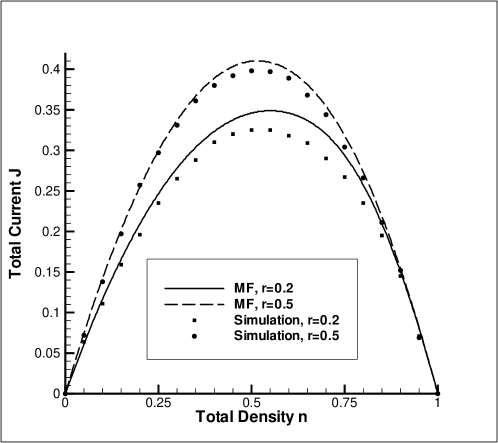
Figure 1: current-density diagram for different values of r. s is set to 0.4 .

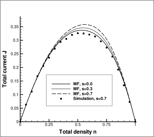
Figure 2: current-density diagrams for different values of s. r is set to 0.2 .

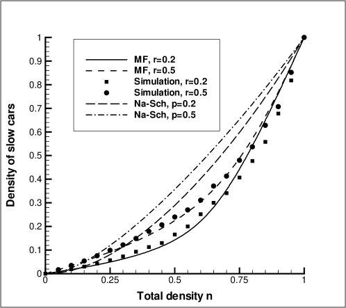
Figure 3: density of slow cars versus the total density for s = 0.4 .

Figure 4: density of slow (fast) cars as a function of r . The values of $n$ and $s$ are 0.2 and 0.4 respectively.

4 Model II

4.1 Asymmetric regulation

The second model we consider, has less resemblance to the Na-Sch model. Here there is no specification of fast and slow cars and only one kind of particle exists in the chain, nevertheless the distinction between fast and slow cars is realized by their appearance in the passing and home-lanes. In this periodic double-chain model the following processes occur in a random sequential updating scheme :

$\circ~{}~{}\circ~{}~{}~{}~{}~{}~{}~{}~{}~{}~{}~{}~{}~{}~{}~{}~{}~{}~{}~{}~{}~{}~{}~{}~{}~{}~{}~{}~{}~{}~{}~{}~{}~{}~{}~{}~{}~{}~{}~{}\circ~{}~{}\circ$
$~{}~{}~{}~{}~{}~{}~{}~{}~{}\longrightarrow~{}~{}~{}~{}~{}~{}~{}{\rm with}\ \ {\rm rate}\ \ h$
$~{}~{}~{}~{}~{}\bullet~{}\circ~{}~{}~{}~{}~{}~{}~{}~{}~{}~{}~{}~{}~{}~{}~{}~{}~{}~{}~{}~{}~{}~{}~{}~{}~{}~{}~{}~{}~{}~{}~{}~{}~{}~{}~{}~{}~{}~{}~{}\circ~{}~{}\bullet$

$\circ~{}~{}\circ~{}~{}~{}~{}~{}~{}~{}~{}~{}~{}~{}~{}~{}~{}~{}~{}~{}~{}~{}~{}~{}~{}~{}~{}~{}~{}~{}~{}~{}~{}~{}~{}~{}~{}~{}~{}~{}~{}~{}\circ~{}~{}\bullet$
$~{}~{}~{}~{}~{}~{}~{}~{}~{}\longrightarrow~{}~{}~{}~{}~{}~{}~{}{\rm with}\ \ {\rm rate}\ \ a$
$~{}~{}~{}~{}~{}\bullet~{}\bullet~{}~{}~{}~{}~{}~{}~{}~{}~{}~{}~{}~{}~{}~{}~{}~{}~{}~{}~{}~{}~{}~{}~{}~{}~{}~{}~{}~{}~{}~{}~{}~{}~{}~{}~{}~{}~{}~{}~{}\circ~{}~{}\bullet$

$\bullet~{}~{}\circ~{}~{}~{}~{}~{}~{}~{}~{}~{}~{}~{}~{}~{}~{}~{}~{}~{}~{}~{}~{}~{}~{}~{}~{}~{}~{}~{}~{}~{}~{}~{}~{}~{}~{}~{}~{}~{}~{}~{}\circ~{}~{}\circ$
$~{}~{}~{}~{}~{}~{}~{}~{}~{}~{}\longrightarrow~{}~{}~{}~{}~{}~{}~{}{\rm with}\ \ {\rm rate}\ \ g$
$~{}~{}~{}~{}~{}\bullet~{}\circ~{}~{}~{}~{}~{}~{}~{}~{}~{}~{}~{}~{}~{}~{}~{}~{}~{}~{}~{}~{}~{}~{}~{}~{}~{}~{}~{}~{}~{}~{}~{}~{}~{}~{}~{}~{}~{}~{}~{}\bullet~{}~{}\bullet$

$\bullet~{}~{}\circ~{}~{}~{}~{}~{}~{}~{}~{}~{}~{}~{}~{}~{}~{}~{}~{}~{}~{}~{}~{}~{}~{}~{}~{}~{}~{}~{}~{}~{}~{}~{}~{}~{}~{}~{}~{}~{}~{}~{}\circ~{}~{}\bullet$
$~{}~{}~{}~{}~{}~{}~{}~{}~{}~{}~{}\longrightarrow~{}~{}~{}~{}~{}~{}~{}{\rm with}\ \ {\rm rate}\ \ b$
$~{}~{}~{}~{}~{}\bullet~{}\bullet~{}~{}~{}~{}~{}~{}~{}~{}~{}~{}~{}~{}~{}~{}~{}~{}~{}~{}~{}~{}~{}~{}~{}~{}~{}~{}~{}~{}~{}~{}~{}~{}~{}~{}~{}~{}~{}~{}~{}\bullet~{}~{}\bullet$

As depicted, the ”asymmetric ” regulation has been adopted so that the top-lane can only be used for passing. According to the above rules, once a successful passing has taken place, the passing car should return to its home-lane unless the next site in the home-lane is already occupied. In this circumstance, it can continue to pass the second slow car ( multi-passing ). Each site of the double chain takes four different states but according to the above dynamics only three of them appears in the course of time. The forbidden state is the one in which the passing-lane site is full and its parallel home-lane site is empty. Regarding this fact, we characterize the three allowed states by $\Phi,A$ and $B$. $\Phi$ represents the situation where both parallel sites are empty, $A$ represents the case of an occupied site in the home-lane and empty parallel site in passing-lane and finally $B$ refers to the case of both parallel sites being occupied.

This notation yields the following reaction-diffusion processes:

$$A~{}\Phi\rightarrow\Phi~{}A\ \ \ ({\rm with}\ \ {\rm rate}\ \ h)$$ (18)

$$A~{}A\rightarrow\Phi~{}B\ \ \ ({\rm with}\ \ {\rm rate}\ \ a)$$ (19)

$$B~{}\Phi\rightarrow A~{}A\ \ \ ({\rm with}\ \ {\rm rate}\ \ g)$$ (20)

$$B~{}A\rightarrow A~{}B\ \ \ ({\rm with}\ \ {\rm rate}\ \ b)$$ (21)

It is worth mentioning that the above model for a two-lane road is simultaneously being considered within the approach of Deterministic Cellular Automata (DCA) [25].

4.2 Master equation and mean-field approach

Similar to the steps performed in model I, one can write the following form of discrete continuity equation.

$${d\over dt}\left[\langle n_{k,A}\rangle+2\langle n_{k,B}\rangle\right]=\langle J_{k}^{in}\rangle-\langle J_{k}^{out}\rangle$$ (22)

in which

$$\langle J_{k}^{out}\rangle=h\langle n_{k,A}e_{k+1}\rangle+b\langle n_{k,B}n_{k+1,A}\rangle+g\langle n_{k,B}e_{k+1}\rangle+a\langle n_{k,A}n_{k+1,A}\rangle$$ (23)

The above expression for $\langle J_{k}\rangle$ has a clear interpretation in terms of rules (18-21). In steady state, the time dependences in the equation disappear and the current will be site-independent. Next we apply the mean-field approximation through which all the two-point correlators are replaced by the product of one-point correlators. This leads to the following equation for $J$:

$$J=hn_{A}(1-n)+b(n-{n_{A}\over 2})n_{A}+g(n-{n_{A}\over 2})(1-n)+an_{A}^{2}$$ (24)

where the relation ${n_{A}\over 2}+n_{B}=n$ has been used.
In order to obtain $J$ in terms of total density $n$ and the rates, we must write $n_{A}$ as a function of $n$ and the rates. This is done by solving the following equation with its left hand side set to zero.

$${d\over dt}n_{A}=2gn_{B}(1-n)-2an_{A}^{2}$$ (25)

The unique physical solution of the above equation is:

$$n_{A}={1\over 4a}\left[\{(g^{2}(1-n)^{2}+16an(1-n)g)\}^{{1\over 2}}-g(1-n)\right]$$ (26)

putting (26) in the eq. (24), the current $J$ is now obtained in terms of $n$ and the rates. The result of computer simulations are shown in the following set of figures. Here the rate $b,g$ and $h$ are chosen to be $1.0,1.0$ and $0.7$ respectively while $a$ is varied. We recall that ”$a$” measures the tendency of fast cars to pass the slow ones.The simulation specifications are the same as those in model I.

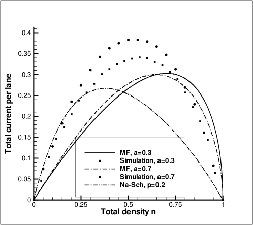
Figure 5: current-density diagram for different values of passing rate.

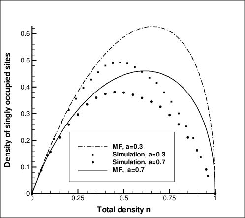
Figure 6: density of singly occupied sites versus the total density

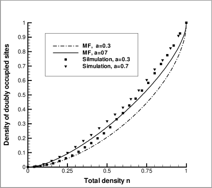
Figure 7: density of doubly-occupied sites versus the total density.

4.3 Symmetric Regulation

Here we allow the fast cars to pass rightward as well. In this case, both the top and bottom lanes become identical and fast cars can pass the slow ones irrespective of their home-lane. In this symmetric two-lane model, each particle hops one site ahead in its home-lane provided that the next site is empty. Otherwise it tries to pass the car ahead. This attempt is successful if there is an empty site ahead on the opposite lane. The following rules illustrates the model definition.

$\ast~{}~{}\ast~{}~{}~{}~{}~{}~{}~{}~{}~{}~{}~{}~{}~{}~{}~{}~{}~{}~{}~{}~{}~{}~{}~{}~{}~{}~{}~{}~{}~{}~{}~{}~{}~{}~{}~{}~{}~{}~{}~{}\ast~{}~{}\ast$
$~{}~{}~{}~{}~{}~{}~{}~{}~{}\longrightarrow~{}~{}~{}~{}~{}~{}~{}{\rm with}\ \ {\rm rate}\ \ h$
$~{}~{}~{}~{}~{}\bullet~{}\circ~{}~{}~{}~{}~{}~{}~{}~{}~{}~{}~{}~{}~{}~{}~{}~{}~{}~{}~{}~{}~{}~{}~{}~{}~{}~{}~{}~{}~{}~{}~{}~{}~{}~{}~{}~{}~{}~{}~{}\circ~{}~{}\bullet$

$\bullet~{}~{}\circ~{}~{}~{}~{}~{}~{}~{}~{}~{}~{}~{}~{}~{}~{}~{}~{}~{}~{}~{}~{}~{}~{}~{}~{}~{}~{}~{}~{}~{}~{}~{}~{}~{}~{}~{}~{}~{}~{}~{}\circ~{}~{}\bullet$
$~{}~{}~{}~{}~{}~{}~{}~{}~{}\longrightarrow~{}~{}~{}~{}~{}~{}~{}{\rm with}\ \ {\rm rate}\ \ h$
$~{}~{}~{}~{}~{}\ast~{}\ast~{}~{}~{}~{}~{}~{}~{}~{}~{}~{}~{}~{}~{}~{}~{}~{}~{}~{}~{}~{}~{}~{}~{}~{}~{}~{}~{}~{}~{}~{}~{}~{}~{}~{}~{}~{}~{}~{}~{}\ast~{}~{}\ast$

$\bullet~{}~{}\bullet~{}~{}~{}~{}~{}~{}~{}~{}~{}~{}~{}~{}~{}~{}~{}~{}~{}~{}~{}~{}~{}~{}~{}~{}~{}~{}~{}~{}~{}~{}~{}~{}~{}~{}~{}~{}~{}~{}~{}\circ~{}~{}\bullet$
$~{}~{}~{}~{}~{}~{}~{}~{}~{}~{}\longrightarrow~{}~{}~{}~{}~{}~{}~{}{\rm with}\ \ {\rm rate}\ \ g$
$~{}~{}~{}~{}~{}\circ~{}\circ~{}~{}~{}~{}~{}~{}~{}~{}~{}~{}~{}~{}~{}~{}~{}~{}~{}~{}~{}~{}~{}~{}~{}~{}~{}~{}~{}~{}~{}~{}~{}~{}~{}~{}~{}~{}~{}~{}~{}\circ~{}~{}\bullet$

$\circ~{}~{}\circ~{}~{}~{}~{}~{}~{}~{}~{}~{}~{}~{}~{}~{}~{}~{}~{}~{}~{}~{}~{}~{}~{}~{}~{}~{}~{}~{}~{}~{}~{}~{}~{}~{}~{}~{}~{}~{}~{}~{}\circ~{}~{}\bullet$
$~{}~{}~{}~{}~{}~{}~{}~{}~{}~{}~{}\longrightarrow~{}~{}~{}~{}~{}~{}~{}{\rm with}\ \ {\rm rate}\ \ g$
$~{}~{}~{}~{}~{}\bullet~{}\bullet~{}~{}~{}~{}~{}~{}~{}~{}~{}~{}~{}~{}~{}~{}~{}~{}~{}~{}~{}~{}~{}~{}~{}~{}~{}~{}~{}~{}~{}~{}~{}~{}~{}~{}~{}~{}~{}~{}~{}\circ~{}~{}\bullet$
The astrix symbol indicates that the process in the opposite lane occurs independently of the configuration of the sites filled with astrix. If we denote the state of two parallel sites in which the bottom site is empty and the top one is occupied by $B$, the state of simultaneous occupation of parallel sites by $C$ and adopting the notations $\Phi$ and A as the same in the asymmetric version of the model, then it could easily be verified that the forms of the discrete continuity equation and the current are as follows:

$${d\over dt}\left(\langle a_{k}\rangle+\langle b_{k}\rangle+2\langle c_{k}\rangle\right)=\langle J_{k-1}\rangle-\langle J_{k}\rangle$$ (27)

and
$\langle J_{k,k+1}\rangle=h\left(\langle a_{k}e_{k+1}\rangle+\langle a_{k}b_{k+1}\rangle+2\langle c_{k}e_{k+1}\rangle+\langle c_{k}b_{k+1}\rangle+\langle b_{k}e_{k+1}\rangle+\langle b_{k}a_{k+1}\rangle+\langle c_{k}a_{k+1}\rangle\right)$

$$+g\left(\langle b_{k}b_{k+1}\rangle+\langle a_{k}a_{k+1}\rangle\right)$$ (28)

Where $\langle a_{k}\rangle,\langle b_{k}\rangle$ and $\langle c_{k}\rangle$ refer to the probabilities that at time $t$, the site $N=k$ of the double-chain has one car in bottom lane, one car in top lane and double-occupancy in both lanes respectively. In steady state, the system is both time and site independent. Denoting the steady values of $\langle a_{k}\rangle,\langle b_{k}\rangle$ and $\langle c_{k}\rangle$ by $a,b$ and $c$, one has the relation:

$${a+b\over 2}+c=n$$ (29)

Moreover, the symmetry between the lanes implies that $a=b$. The steady value $a$ is easily found to be obtained from the following equation:

$$(g+h)a^{2}=hc(1-n)$$ (30)

Solving the steady-state equation for $a$, one finds:

$$a={(\left[h^{2}(1-n)^{2}+4hn(1-n)(g+h)\right])^{{1\over 2}}-h(1-n)\over 2(g+h)}$$ (31)

Also equation (31) leads to the following equation for $J$.

$$J=2\left[hn(1-n)+h\{a^{2}+2a(n-a)\}+ga^{2})\right]$$ (32)

Where by putting the eq. (31) into it, one reaches to expression for $J$ in terms of $n,g$ and $h$. We remark that the factor two reflects the number of lanes. The result of computer simulations are shown in the following set of figures. The value of $h$ is set to one and $g$ is varied.

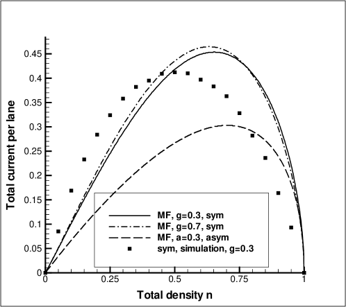
Figure 8: current per lane-density diagram for different values of passing rates

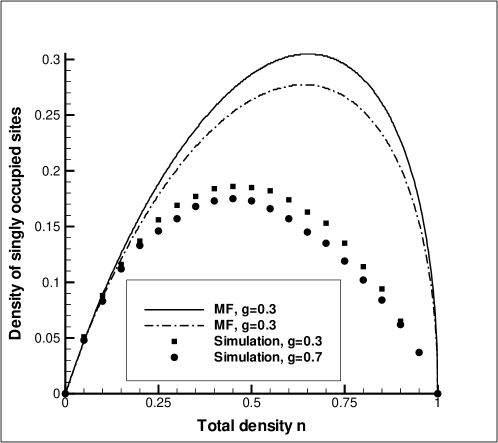
Figure 9: density of singly occupied sites versus the total density.

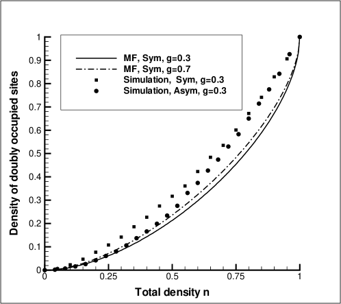
Figure 10: density of doubly occupied sites versus the total density.

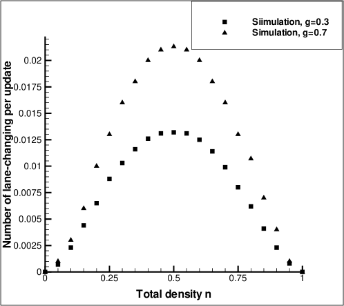
Figure 11: number of lane-changing per update versus total density.

5 Concluding Remarks

We have introduced a two-species reaction-diffusion model for description of a uni-directional two-lane road. The type of update we have used is random-sequential which sounds more appropriate for analytical treatments. In the first model, the result of numeric simulations are very close to those in mean-field approach which indicates that the effects of correlations are suppressed. However in the second model, there are remarkable differences between analytical and numeric results. in model I, the current-density diagram is slightly affected by changing the passing rate and the passing process has its most effect in the intermediate densities. This could be anticipated since in the low and high densities the number of passing considerably reduces. The space-time diagrams of the model I reveal the discriminating effect of passing.
In model II (both symmetric and asymmetric), the maximum of $J$ occurs in different values of $n$ in simulation and analytical approach. Mean-field predicts a shift toward higher densities while in simulation a slight shift toward left is observed. We note that in the PCA based models the maximum of $J$ corresponds to a considerable left-shifted value of the density [16, 17]. In symmetric version of the model II, we observe an increment of the current with regard to the asymmetric version. In contrast to the asymmetric version, the maximum of $J$ in mean-field approach is higher than its value obtained through simulation. Although the current diagram (10) appears asymmetrically with respect to the density, the lane-changing diagram (13) is symmetric to a high accuracy.

Acknowledgements:
I would like to express my gratitude to V. Karimipour and G. Schütz, for their fruitful comments. I acknowledge the assistance given by A. Schadschneider, N.Hamadani, V.Shahrezaei, R. Sorfleet and in particular I highly appreciate R. Gerami for his valuable helps in the computer simulations.

References

- [1] D. Chowdhury, L. Santen and A. Schadschneider, Statistical physics of vehicular traffic and some related systems, to appear in Phys.Reports 2000
- [2] D.E. Wolf, M. Schreckenberg and A. Bachem (eds) Traffic and granular flow (World Scientific, Singapore, 1996).
- [3] D.E Wolf and M. Schreckenberg (eds.) Traffic and granular flow (Springer, Singapore, 1998).
- [4] H.J. Herrmann, D. Helbing, M. Schreckenberg and D.E. Wolf (eds.) Traffic and Granular flow (Springer, Berlin, 2000).
- [5] D. Helbing, Verkehrsdynamik , Springer, Berlin (1998).
- [6] L.A. Pipes, J. Appl. Phys , 24, 274, 1953.
- [7] M.Bando, K.Hasebe, A.Nakayama, A.Shibata and Y.Sugiyama, Jap.J. Indust.Appl.Math, 11, 203, 1994.
- [8] B.S. Kerner, S.L. Klenov and P. Konhaüser, Phys. Rev. E56, 4200, 1997.
- [9] H.Y. Lee, H.-W Lee and D. Kim, Phys. Rev. E59, 5101, 1999.
- [10] I. Prigogine and R. Herman, Kinetic theory of vehicular traffic (Elsevier, Amsterdam, 1971).
- [11] D. Helbing and M. Treiber, Science, 282, 2002, 1998.
- [12] M. Schreckenberg, A. Schadschneider, K. Nagel and N. Ito, Discrete stochastic models for traffic flow, Phys. Rev. E51, 2939 (1995).
- [13] A. Schadshneider, Eur. Phys. J. B , 10 , 573 (1999).
- [14] L. Santen, Numerical Investigation of Discrete Models for Traffic Flow , Dissertation, Universität zu Köln.
- [15] K. Nagel and M. Schreckenberg, J. Physique I, 2, 2221, 1992.
- [16] M. Rickert, K. Nagel, M. Schreckenberg and A. Latour, Physica A 231, 534, 1996.
- [17] K. Nagel, D.E. wolf, P. Wagner and P. Simon, Phys. Rev. E58, 1425, 1998.
- [18] P.M. Simon and H.A. Gutowitz, Phys. Rev. E57 , 2441 (1998).
- [19] K. Nagel, J. Esser and M. Rickert, in Annu. Rev. Comp. Phys. vol VIII, ed. D. Stauffer (World Scientific, March 2000).
- [20] D. Chowdhury and A. Schadschneider, Phys. Rev. E59 , R 1311 (1999).
- [21] T. Nagatini, J. Phys. A: Math Gen. , 29, 6531 (1996).
- [22] G.M. Schütz, Exactly solvable models for many-body systems far from equilibrium, to appear in Phase Transitions and Critical Phenomena, C. Domb and J. Lebowitz (eds.) (academic Press, London, 2000).
- [23] V. Privman(ed), Non-equilibrium Statistical Mechanics in One Dimension , Cambridge University Press, 1997.
- [24] F.C. Alcaraz, M. Droz, M. Henkel and V. Rittenberg, Ann. Phys. (NY), 230 , 250, 1994.
- [25] V. Belitsky, J. Krug, E. Jordao and G.M. Schuẗz, in preparation.