Non-Fermi Liquid Behavior in U and Ce Alloys: Criticality, Disorder, Dissipation, and Griffiths-McCoy singularities.

Abstract

In this paper we provide the theoretical basis for the problem of Griffiths-McCoy singularities close to the quantum critical point for magnetic ordering in U and Ce intermetallics. We show that the competition between Kondo effect and RKKY interaction can be expressed in Hamiltonian form and the dilution effect due to alloying leads to a quantum percolation problem driven by the number of magnetically compensated moments. We argue that the exhaustion paradox proposed by Nozières is explained when the RKKY interaction is taken into account. We revisited the one impurity and two impurity Kondo problem and showed that in the presence of particle-hole symmetry breaking operators the system flows to a line of fixed points characterized by coherent (cluster like) motion of the spins. Moreover, close to the quantum critical point clusters of magnetic atoms can quantum mechanically tunnel between different states either via the anisotropy of the RKKY interaction or by what we call the cluster Kondo effect. We calculate explicitly from the microscopic Hamiltonian the parameters which appear in all the response functions. We show that there is a maximum number $N_{c}$ of spins in the clusters such that above this number tunneling ceases to occur. These effects lead to a distribution of cluster Kondo temperatures which vanishes for finite clusters and therefore leads to strong magnetic response. From these results we propose a dissipative quantum droplet model which describes the critical behavior of metallic magnetic systems. This model predicts that in the paramagnetic phase there is a crossover temperature $T^{*}$ above which Griffiths-McCoy like singularities with magnetic susceptibility, $\chi(T)\propto T^{-1+\lambda}$, and specific heat $C_{V}(T)\propto T^{\lambda}$ with $\lambda<1$ appear. Below $T^{*}$, however, a new regime dominated by dissipation occurs with divergences stronger than power law: $\chi(T)\propto 1/(T\ln(1/T))$ and $C_{V}(T)\propto 1/\ln^{2}(1/T)$. We estimate that $T^{*}$ is exponentially small with $N_{c}$. Our results should be applicable to a broad class of metallic magnetic systems which are described by the Kondo lattice Hamiltonian.

I Introduction

In this paper we are interested in the quantum critical behavior of alloys of actinides and rare earths with metallic atoms. There is a large number of these alloys and they can be classified into two main groups accordingly to their chemical composition: 1) Kondo hole systems which are made out of the substitution of the rare earth or actinide (R) by a non-magnetic metallic atom (M) with a chemical formula R_1-xM_x (a typical example is U_1-xTh_xPd₂Al₃); 2)Ligand systems where one of the metallic atoms (M1) is replaced by another (M2) but the rare earths or actinides are not touched and thus have the formula R(M1)_1-x(M2)_x (as, for instance, UCu_5-xPd_x). In most of these alloys one usually has an ordered magnetic phase at $x=0$ which is destroyed at some critical value $x=x^{*}$ with a non-Fermi liquid (NFL) phase in the vicinity where strong deviations from the predictions of Landau’s theory of the Fermi liquid are observed (see Fig.1). In this paper we propose that the origin for the NFL behavior is the existence of Griffiths-McCoy singularities at low temperatures. As we explain below, these singularities have their origin in a quantum percolation problem driven by the number of magnetically compensated moments. In this percolation problem magnetic clusters can tunnel in the presence of a metallic environment which produces dissipation.

On the one hand, at $x=1$ a Kondo hole system becomes an ordinary Fermi liquid with a temperature independent specific heat coefficient, $\gamma(T)=C_{V}/T$, (by low temperature we mean $T\ll E_{F}$ where $E_{F}$ is the Fermi energy of the metal), the magnetic susceptibility is paramagnetic and given by Pauli’s expression, $\chi(T)=\chi_{0}$, and the resistivity has the Fermi liquid form $R(T)=R_{0}+AT^{2}$. On the other hand, at large $x$ a ligand system is usually a heavy fermion [1], that is, it can also be described by the Fermi liquid expressions but with coefficients $\gamma$ and $\chi_{0}$ orders of magnitude larger than in ordinary metals. The nature of this heavy fermion behavior can be tracked down to the presence of the rare earths or actinides in the alloy. In the NFL phase the specific heat coefficient and the magnetic susceptibility show divergent behavior as the temperature is lowered.

The root for the understanding of the problem lies on the fact that in Landau liquids the thermodynamic and response functions are always well behaved functions of the temperature. This is clearly inconsistent with the behavior in the paramagnetic phase close to a quantum critical point (QCP). Exactly at the QCP divergences are expected since the system is ordering magnetically, thus, QCP can generate NFL behavior [2, 3] (albeit with fine tuning of the chemical composition). It turns out, however, that many times NFL behavior is observed away from the QCP and inside of the paramagnetic phase. One possibility is that the NFL behavior is due to single ion physics and therefore not at all related to the QCP physics. Another possibility is that there are still “traces” of the QCP inside of the paramagnetic phase. This is possible in the presence of disorder which can “pin” pieces of the ordered phase even in the absence of long range order. It is even conceivable that single ion physics and critical behavior co-exist close to a QCP. There is no clear consensus among researchers on the nature of this NFL behavior and the scientific debate is intense. The objective of this work is to shed light into this controversy.

We organize the paper in the following fashion: Section II briefly reviews the problem of NFL behavior in U and Ce intermetallics; in Section III we write an effective Hamiltonian where Kondo effect and RKKY interaction appear explicitly and we discuss the problem of magnetic ordering and dilution within this Hamiltonian; Section IV contains a detailed discussion of the one impurity and two impurity Kondo problem and the extension of the problem to $N$ spin clusters where we define a Kondo cluster effect; in Section V we propose the dissipative quantum droplet model which is the basis for the description of the problem of magnetic ordering in metallic magnetic alloys and we show that at low temperatures dissipation dominates the behavior of the system leading to universal logarithmic divergences, and that at higher temperatures non-universal power law behavior is expected; in Section VI we study the intermediate temperature range where quantum Griffiths singularities are expected; Section VII contains our conclusions. We also have included a few appendices with detailed calculations of the results used in the paper.

II NFL behavior in U and Ce intermetallics

The basis for the study of metals in the last 50 years has been Landau’s theory of the interacting Fermi gas [4]. As consequences of Landau’s theory the thermodynamic and response functions of the electron fluid are smooth functions of the temperature. The magnetic susceptibility has the form (we use units such that $\hbar=k_{B}=1$)

$$\chi(T)=\frac{(g\mu_{B})^{2}N(0)}{4(1+F^{a}_{0})}\,,$$ (1)

where $g\approx 2$ is the Landé factor for the electron, $\mu_{B}$ is the Bohr magneton, $F_{0}^{a}$ is an antisymmetric Landau parameter,

$$N(0)=\frac{m^{*}k_{F}}{\pi^{2}}=\frac{3\rho_{e}}{2E_{F}}\,,$$ (2)

is the density of states at the Fermi energy, $m^{*}$ is the effective mass of the quasiparticles (the effective mass is related to the bare mass, $m$, by a symmetric Landau parameter: $m^{*}/m=1+F^{s}_{1}/3$),

$$k_{F}=(3\pi^{2}\rho_{e})^{1/3}\,,$$ (3)

is the Fermi momentum, $\rho_{e}$ is the number of electrons per unit of volume and $E_{F}=k_{F}^{2}/(2m^{*})$. Moreover, the electronic specific heat, $C_{V}$, is given by the Fermi liquid expression

$$\frac{C_{V}}{T}=\gamma(T)=\frac{\pi^{2}N(0)}{3}\,.$$ (4)

Naturally these expressions resemble the ones obtained for the free electron gas where the bare mass $m$ is replaced by the effective mass $m^{*}$ and Landé factor is renormalized by a factor of $1/\sqrt{1+F^{a}_{0}}$. Furthermore, at low temperatures one expects the electronic resistivity to behave like [5]

$$R(T)=R_{0}+AT^{2}$$ (5)

where $R_{0}$ is the resistivity due to impurities and $A$ is a constant. In a magnetic alloy where the magnetic moments are decoupled from the conduction electrons and do not interact directly among each other we expect an ordinary paramagnetic behavior for the susceptibility in the low field limit ($T\gg g\mu_{B}H$ where $H$ is an applied magnetic field)

$$\chi(T)=\frac{{\cal C}}{T}$$ (6)

where ${\cal C}=\rho_{f}S(S+1)(g\mu_{B})^{2}/3$ is the Curie constant ($\rho_{f}$ is the number of magnetic atoms per unit of volume, $S$ is the magnetic angular momentum of the atom). At low enough temperatures ($T\ll g\mu_{B}H$) the susceptibility vanishes.

The effect of disorder in ordinary Fermi liquids has been studied in great detail [6] and it was found that the results quoted above, especially the temperature dependences of the physical quantities, do not change appreciably (at least when disorder is weak enough to be treated in perturbation theory). Therefore, for a metallic system where Anderson localization [7] does not play a role we still expect Fermi liquid behavior to be a robust feature. Thus, it is indeed very surprising that for such a broad class of U and Ce alloys (which clearly show three-dimensional behavior) deviations from Landau’s theory are so abundant.

In NFL systems it is usually observed that even in the paramagnetic phase the specific heat coefficient and the magnetic susceptibility do not saturate as expected from the Landau scenario. In all the cases studied so far the data for the susceptibility and specific heat have been fitted to weak power laws or logarithmic functions [8]. The resistivity of the systems discussed here can be fitted with $R(T)=R_{0}+AT^{\alpha}$ where $\alpha<2$. Neutron scattering experiments in UCu_5-xPd_x [9] show that the imaginary part of the frequency dependent susceptibility, $\Im(\chi(\omega))$, has power law behavior, that is, $\Im(\chi(\omega))\propto\omega^{1-\lambda}$ with $\lambda\approx 0.7$, over a wide range of frequencies (for a Fermi liquid one expects $\lambda=1$). Moreover, consistent with this behavior the static magnetic susceptibility seems to diverge with $T^{-1+\lambda}$ at low temperatures [8]. What is interesting about UCu_5-xPd_x is that it has been shown in recent EXAFS experiments that this compound has a large amount of disorder [10] consistent with early NMR and $\mu$SR experiments [11].

From the magnetic point of view the U and Ce intermetallics show a rich variety of magnetic ground states: antiferromagnetic as in the case of UCu_5-xPd_x for $0\leq x\leq 1$ [9], ferromagnetic as in the case of U_1-xTh_xCu₂Si₂ for $0.6\leq x\leq 0.85$ [12] and spin glass as in the case of U_1-xY_xPd₃ for $0.6\leq x\leq 0.8$ [13]. There are many indications that the magnetism in these alloys is inhomogeneous with strong coupling to the lattice. This seems to be the case of CeAl₃ [14] or CePd₂Al₃ [15] where $\mu$SR experiments have shown clear signs of microscopic inhomogeneity. Moreover, because of the strong spin-orbit coupling in these systems a myriad of magnetic states with different ordering configurations are found [16].

On the theoretical side [16] we can classify the approaches to NFL as of single ion character or cooperative behavior. Single impurity approaches for the NFL problem are very important because the Kondo effect [17] has been suggested as the source of heavy fermion behavior [1] in undiluted ligand systems (say, CeAl₃) [18]. Nozières and Blandin proposed the multichannel Kondo effect [19] as a possible source of NFL behavior. D. Cox proposed that such a multichannel effect of quadrupolar origin should exist in these systems [20]. Another source of NFL behavior based on single impurity physics is the so-called Kondo disorder approach which postulates an a priori broad distribution of single ion Kondo temperatures [11, 21]. The cooperative approaches, on the other hand, stress the proximity to a critical point as a source of NFL behavior and was pioneered by Hertz [2, 3] and has been applied to many of the systems we discuss here [22, 23, 24, 25, 26]. The problem of disorder close to the QCP has been discussed by many authors over the years. Hertz studied a classical XY model and showed that disorder is a relevant perturbation [27] in dimensions smaller than $4$. Bhatt and Fisher [28] and more recently Sachdev [29] have argued that for Hubbard-like models an instability to a inhomogeneous phase should exist close to the QCP. A more recent work extending Hertz calculations to the case of disorder has reached similar conclusions, namely, that close to the QCP a new type of critical behavior, very different from the critical behavior of the clean system, should exist [30].

It is clear from the experimental and theoretical point of view that magnetic interactions and the Kondo effect should be relevant for the physics of U and Ce intermetallics. Moreover, it has been claimed for a long time that it is the competition between Kondo effect and magnetic order that determines the phase diagram of these systems. This idea was put forward by Doniach [31] and we discuss it in more detail below. In trying to reconciliate the Doniach argument with the existence of disorder in these systems we proposed recently a new explanation for the NFL behavior in these systems which is based on the magnetic inhomogeneity due to this competition. In other words, if the Kondo effect is responsible for the destruction of long range order in the magnetically ordered system then at the QCP the competition between magnetic ordering and magnetic quenching is strongest [32]. We have argued that close to the QCP, in the paramagnetic phase, finite clusters of magnetically ordered atoms can fluctuate quantum mechanically. In this case a so-called quantum Griffiths-McCoy singularities would be generated and zero temperature divergences of the physical quantities should be observed. In the next sections we explain exactly how this process occurs.

Classical Griffiths singularities appear in the context of classical Ising models as due to the response of rare and large clusters to an external magnetic field [33]. A classical model with columnar disorder was solved exactly by McCoy and Wu [34] in two dimensions and shows clearly the importance of Griffiths singularities close to the critical point for magnetic order. There are indeed experimental indications for the existence of such singularities in Fe_0.47Zn_0.53F₂ and other Ising magnets [35]. Because of the relationship between the classical statistical mechanics in $d$ dimensions and the quantum statistical mechanics in $d+1$ dimensions the McCoy-Wu model can be mapped at $T=0$ into the transverse field Ising model which has been studied by D. Fisher [36]. The transverse field Ising model is supposed to be applicable to insulating magnets since conduction electron degrees of freedom are not present. Senthil and Sachdev have studied the transverse field Ising model in higher dimensions on a percolating lattice and have found that quantum Griffiths singularities should be present in the paramagnetic phase in these systems close to the QCP [37]. Moreover, many physical quantities diverge at zero temperature as a result of the strong response of the large and rare clusters. Such anomalous behavior close to the QCP has been confirmed numerically in dimensions higher than one [38] and there is today strong experimental indication of such behavior in U and Ce intermetallics [39].

III Effective Hamiltonian: RKKY $\times$ Kondo

In our discussion of the physics of U and Ce intermetallics we are going to use the so-called Kondo lattice Hamiltonian which describes the exchange interactions between itinerant electron spins and the localized magnetic moments:

$$H=\sum_{{\bf k},\kappa}\epsilon_{\kappa}({\bf k})c^{{\dagger}}_{{\bf k},\kappa}c_{{\bf k},\kappa}+\sum_{i}\sum_{a,b,\kappa,\kappa^{\prime}}J_{a,b}(i)S^{a}(i)c^{{\dagger}}_{\kappa}(i)\tau_{\kappa,\kappa^{\prime}}^{b}c_{\kappa^{\prime}}(i)$$ (7)

where $\kappa=1,2$ labels the spin states, $J_{a,b}(i)$ are the effective exchange constants between the localized spins and conduction electrons at sites ${\bf r}_{i}$. $S^{a}(i)$ is the localized electron spin operator and $\sum_{\kappa,\kappa^{\prime}}c^{{\dagger}}_{\kappa}(i)\tau_{\kappa,\kappa^{\prime}}^{b}c_{\kappa^{\prime}}(i)$ the conduction electron spin operator where $c_{{\bf k},\kappa}$ annihilates an electron with momentum ${\bf k}$ and spin projection $\kappa$ ($\tau^{b}$ with $a,b=x,y,z$ are Pauli spin matrices). Observe that we are allowing for the possibility of the conduction electron dispersion $\epsilon_{\kappa}({\bf k})$ to be dependent of the electron spin. Indeed, one can show that (7) can be obtained directly from the Anderson Hamiltonian [40] when spin-orbit effects are included and the hybridization energy between localized and itinerant electrons is much smaller than the atomic energy scales [41]. One of the striking features of (7) is the fact that the exchange interaction is not symmetric in spin space because of spin-orbit coupling. As we discuss below besides canted magnetism (7) gives rise to what we call a canted Kondo effect.

The main problem in studying the competition of Rudermann-Kittel-Kasuya-Yosida interaction (RKKY) [42] and Kondo effect in the Hamiltonian (7) is related to the fact that both the RKKY and the Kondo effect have origin on the same magnetic coupling between spins and electrons. What allows us to treat this problem is the fact that the RKKY interaction is perturbative in $J/E_{F}$ while the Kondo effect is non-perturbative in this parameter and requires different techniques. Moreover, the RKKY interaction depends on electronic states deep inside of the Fermi sea, in addition to those at $E_{F}$, while the Kondo effect is purely a Fermi surface effect. Thus, it seems to be possible to use perturbation theory to treat the RKKY interaction.

We will consider, for simplicity the case where the Fermi surfaces for the two species of electrons are spherical. The local electron operator can be written in momentum space as

$$c_{\kappa}(i)=\frac{1}{\sqrt{N}}\sum_{{\bf k}}e^{i{\bf k}\cdot{\bf r}}\,c_{{\bf k},\kappa}\,.$$ (8)

We now separate the states in momentum space into three different regions of energy as shown in Fig.2, namely, $\Omega_{0}$: $k_{F,\alpha}-\Lambda<k<k_{F,\alpha}+\Lambda$; $\Omega_{1}$: $k<k_{F,\alpha}-\Lambda$; and $\Omega_{2}$: $k>k_{F,\alpha}+\Lambda$ where $\Lambda$ is an arbitrary cut-off. As we discuss below the value of the cut-off is related to the number of compensated spins in the system. But for the moment being we consider it as some arbitrary quantity we can vary, like in a renormalization group calculation. Observe that the sum in (8) can also be split into these three different regions. The problem we want to address is how the states in region $\Omega_{0}$ close to the Fermi surface renormalize as one traces out high energy degrees of freedom which are present in regions $\Omega_{1}$ and $\Omega_{2}$. We are going to do this calculation perturbatively in $J/E_{F}$ [43]. For this purpose it is convenient to use a path integral representation for the problem and write the quantum partition function as

$$Z=\int D{\bf S}(n,t)D\overline{\psi}({\bf r},t)D\psi({\bf r},t)\exp\left\{i{\cal S}[{\bf S},\overline{\psi},\psi]\right\}$$ (9)

in terms of Grassman variables $\overline{\psi}$ and $\psi$ and where the path integral over the localized spins also contains the constraint that ${\bf S}^{2}(n,t)=S(S+1)$. The quantum action in (9) can be separated into three different pieces, ${\cal S}={\cal S}_{0}[{\bf S}]+{\cal S}_{0}[\overline{\psi},\psi]+{\cal S}_{I}[{\bf S},\overline{\psi},\psi]$, where ${\cal S}={\cal S}_{0}[{\bf S}]$ is the free actions of the spins (which can be written, for instance, in terms of spin coherent states [44]),

$${\cal S}_{0}[\overline{\psi},\psi]=\sum_{\alpha,\gamma}\int\frac{d\omega}{2\pi}\sum_{\bf k}\overline{\psi}_{\alpha}({\bf k},\omega)\left(\omega+\mu-\epsilon_{\alpha}({\bf k})\right)\delta_{\alpha,\gamma}\psi_{\gamma}({\bf k},\omega)$$ (10)

is the free action for the conduction electrons and

$${\cal S}_{I}[{\bf S},\overline{\psi},\psi]=\int dt\sum_{\alpha,\gamma}\sum_{n}J_{a,b}(n)S_{a}(n,t)\tau^{b}_{\alpha,\gamma}\overline{\psi}_{\alpha}(n,t)\psi_{\gamma}(n,t)$$ (11)

is the exchange interaction between conduction electrons and localized moments. We now split the Grassman fields into the momentum shells defined above, that is, we rewrite the path integral as

$$Z=\int D{\bf S}(n,t)\prod_{i=0}^{2}D\overline{\psi}_{i}({\bf r},t)D\psi_{i}({\bf r},t)\exp\left\{i{\cal S}[{\bf S},\{\overline{\psi}_{i},\psi_{i}\}]\right\}$$ (12)

where the indices $0,1,2$ refer to the degrees of freedom which reside in the momentum regions $\Omega_{0}$, $\Omega_{1}$ and $\Omega_{2}$, respectively. The action of the problem can be rewritten as ${\cal S}={\cal S}_{0}[{\bf S}]+\sum_{i=0}^{2}{\cal S}_{0}[\overline{\psi}_{i},\psi_{i}]+{\cal S}_{I}[{\bf S},\overline{\psi},\psi]$. Notice the free part of the electron action is just a sum of three terms (essentially by definition since the non-interacting problem is diagonal in momentum space). Moreover, the exchange part mixes electrons in all three regions defined above:

$${\cal S}_{I}=\sum_{n}\int dt\sum_{i,i^{\prime}=0}^{2}J_{a,b}({\bf r}_{n})S_{a}({\bf r}_{n},t)\tau^{b}_{\alpha,\gamma}\overline{\psi}_{\alpha,i}({\bf r}_{n},t)\psi_{\gamma,i^{\prime}}({\bf r}_{n},t)\,.$$ (13)

Since we are interested only on the physics close to the Fermi surface we trace out the fast electronic modes in the regions $\Omega_{1}$ and $\Omega_{2}$ assuming that $J_{a,b}\ll\mu$. As we show in Appendix (A), besides the renormalization of the parameters in free action of the electrons in the region $\Omega_{0}$, we get the RKKY interaction between localized moments. The effective action of the problem becomes:

$${\cal S}_{eff}[{\bf S},\overline{\psi}_{0},\psi_{0}] = {\cal S}_{0}[\overline{\psi}_{0},\psi_{0}]+\sum_{n}\int dt\sum_{\alpha,\gamma,a,b}J^{R}_{a,b}({\bf r}_{n})S_{a}({\bf r}_{n},t)\tau^{b}_{\alpha,\gamma}\overline{\psi}_{\alpha,0}({\bf r}_{n},t)\psi_{\gamma,0}({\bf r}_{n},t)$$ (14)

$$+ \sum_{n,m,a,b}\int dt\,\,\Gamma^{R}_{a,b}({\bf r}_{n}-{\bf r}_{m},\Lambda)S_{a}({\bf r}_{n},t)S_{b}({\bf r}_{m},t)$$ (15)

where $\Gamma^{R}_{a,b}({\bf r}_{n}-{\bf r}_{m},\Lambda)$ is the cut-off dependent RKKY interaction between the local moments and $J^{R}_{a,b}(n)$ is the Kondo electron-spin coupling renormalized by the high energy degrees of freedom. As we show in Appendix (A) this renormalization can be calculated exactly. For a spherical Fermi surface the exchange interaction between spins can be written as:

$$\Gamma^{R}_{a,b}(r,\Lambda)=-\frac{9c^{2}\overline{n}}{E_{F}}\sum_{c}J_{a,c}J_{b,c}{\cal F}(2k_{F}r,\Lambda/k_{F})e^{-r/\ell}$$ (16)

where $c$ is the number of magnetic moments per atom, $\overline{n}$ is the number of electrons per atom, $\ell$ is the electron mean-free path and ${\cal F}(x,y)$ is given in (A56). In Fig.3 we compare the usual RKKY with $\Lambda=0$ and the RKKY with finite $\Lambda$. At short distances, $r\ll k_{F}^{-1},\Lambda^{-1}$, the interaction is ferromagnetic and is renormalized by a factor of $(1-\Lambda/k_{F})^{3}$. Moreover, as shown in Fig.4 the first zero of the RKKY interaction is shifted from $k_{F}r\approx 2.2467$ at $\Lambda=0$ to smaller values. At intermediate distances, that is, $\Lambda^{-1}\gg r>k_{F}^{-1}$, the RKKY interaction decays like $1/r^{3}$ as in the case of $\Lambda=0$ but the most striking result is that for large distances, $r>>k_{F}^{-1},\Lambda^{-1}$ the RKKY interactions decays like $1/r^{4}$ instead of the usual $1/r^{3}$. Thus, for finite $\Lambda$ the RKKY interaction has a shorter range. Another interesting result of a finite $\Lambda$ is that at short and intermediate distances the RKKY oscillations are mostly antiferromagnetic. As one can see directly from Fig.3 the ferromagnetic part of the RKKY is suppressed after the first zero. This could perhaps explain why most of the alloys of the type discussed here have antiferromagnetic ground states.

We observe further that the perturbation theory here is well behaved and there are no infrared singularities in the perturbative expansion. Thus, the limit of $\Lambda\to 0$ is well-defined. In this limit $\Gamma^{R}_{a,b}({\bf r}_{n}-{\bf r}_{m},\Lambda\to 0)$ becomes the usual RKKY interaction one would calculate by tracing all the energy shells of the problem. Observe that there are no retardation effects in tracing this high energy degrees of freedom since they are much faster than the electrons close to the Fermi surface and therefore adapt adiabatically to their motion. Hamiltonian (15) is the basic starting point to our approach and contains the basic elements for the discussion of magnetic order in the system. Observe that the RKKY interaction depends on the electronic states far away from the Fermi surface while the Kondo interaction is a pure Fermi surface effect. While the RKKY interaction leads to order of the magnetic moments the Kondo coupling induces magnetic quenching. It is the interplay of these two interaction which leads to the physics we discuss here. The action (15) has been used as a starting point for many theoretical discussions of rare earth alloys [45]. We stress, however, that the action (15) describes only the low energy degrees of freedom of the problem and therefore the exchange constants that appear there can have strong renormalizations due to the high energy degrees of freedom. Moreover, as we explain below the cut-off $\Lambda$ depends on the number of compensated moments.

A Magnetically ordered phase: the role of RKKY

The existence of local moments is not a sufficient condition for the existence of long range magnetic order. It is exactly the interaction between the spins which determines the ordering temperature $T_{c}$ of the material. There are various ways localized moments can interact: dipolar-dipolar interactions, kinetic exchange interactions due to the overlap of the f orbitals and RKKY interaction. Dipolar interactions are too small to account for the ordering temperature in these systems (they range from $100$ K down to $10$ K in the pure compounds) and the direct exchange between f orbitals is very weak since the spatial extent of the f orbitals is small (with the possible exception of the 5f orbitals of U). The RKKY interaction is by far the most important interactions in metallic rare earth alloys and it will be the only interaction we will consider in detail.

As it is well-known and as shown in Appendix A in the ordered case ($\Lambda=0$) the RKKY interaction decays like $1/r^{3}$ and oscillates in real space with wave-vector $2k_{F}$. The oscillatory terms have to do with the sharpness of the Fermi surface. Moreover, non-spherical Fermi surfaces will also lead to an angular dependence on the RKKY interaction with decaying rates which vary with the direction [46]. The specific form of the RKKY interaction is not important in our discussion but the fact that the RKKY is an interaction which is perturbative in $J/\mu$ and scales like $N(0)J^{2}$. The exponential factor due to disorder was obtained originally by de Gennes [47].

Observe that the spin-orbit coupling generates an RKKY interaction which is anisotropic and therefore can give rise to canted magnetism. This effect is the analogue of the anisotropic spin exchange interaction, or Dzyaloshinsky-Moriya (DM) exchange interaction [48] in insulating magnets which is obtained via the kinetic exchange between localized moments in the presence of spin-orbit coupling. The interaction (16) is an indirect exchange interaction in the presence of spin-orbit coupling. Thus, as in the case of DM interactions one expects parasitic ferromagnetism within antiferromagnetic phases. This effect has been observed long ago in R-Cr0₃ systems[49, 50]. The existence of ferromagnetic and antiferromagnetic coupling creates a very rich situation where many different magnetic phases are possible in the presence of a Lifshitz point [51]. Recent theoretical approaches for the NFL problem in CeCu_6-yAu_y are based on the idea that the Lifshitz point in these systems is a QCP [23] and therefore the quantum fluctuations associated with this point induce NFL behavior in the conduction band.

The critical temperature of the system can be estimated directly from the mean field theory for (7) and it is given by [52]

$$T_{c}=\frac{2S(S+1)}{3}\sum_{{\bf R}\neq 0}\Gamma_{M}({\bf R})\cos\left({\bf Q}\cdot{\bf R}\right)$$ (17)

where ${\bf Q}$ is the ordering vector ($Q=0$ for ferromagnetism) and $\Gamma_{M}({\bf R})$ is the largest eigenvalue of $\Gamma_{a,b}({\bf R})$. Observe that $T_{c}$ scales with $\Gamma$ and therefore it is proportional to $N(0)J^{2}$. This value of $T_{c}$ gives the order of magnitude of the transition temperature in Kondo hole or ligand systems, that is, the magnetically ordered Kondo lattice. In what follows we discuss the effect of disorder on the magnetic order in these systems.

B Magnetic dilution

In Kondo hole systems the transition to the paramagnetic phase happens because the magnetic sublattice is diluted with non-magnetic atoms. In this case two main effects occur: (1) the magnetic system loses its magnetic atoms; (2) because the non-magnetic atoms do not have the same size of the magnetic ones there is a local lattice contraction or expansion. The first effect created by the dilution is to introduce disorder in the electronic environment and produce a finite scattering time $\tau$ for the electron. As shown by de Gennes long ago [47], the RKKY interaction decays exponentially with the electron mean-free path, $\ell=v_{F}\tau$. Notice that this is only true if there is true magnetic long range order in the problem. In the case of a spin glass order this is argument is not correct [53].

The problem of destruction of magnetic order in a ligand system is more complex since the magnetic atoms are not replaced. In an alloy like UCu_4-xPd_x the Cu atoms are replaced by the somewhat smaller Pd atoms. This difference between the Pd and the Cu leads to a local lattice contraction which modifies the local hybridization matrix elements. Since these matrix elements are exponentially sensitive to the overlap between different angular momentum orbitals one can have large local effects in the system. This change of local matrix elements induces changes in the exchange constants between the conduction band and the localized moments, $J({\bf r}_{i})$, in (7).

Let us start with (7) and in the homogeneous ordered phase where we assume that $J_{a,b}({\bf r}_{i})=J_{a,b}$ for all sites. The transition temperature is given by (17) with $\Gamma$ given by (16) with the electron mean free path determined by the extrinsic impurities in the system. As the Kondo lattice is doped, either by substitution of a magnetic atom by a non-magnetic one (as in the case of the Kondo hole systems) or just disordered (as in the case of ligand systems) the local coupling between the localized moments and electrons is changed from $J_{a,b}$ to a different value $\tilde{J}_{a,b}$ (for simplicity we will assume just a binary distribution but this assumption can be easily generalized). In this case can rewrite (7) as $H=H_{0}+H_{KL}+H_{imp}$ where:

$$H_{0} = \sum_{{\bf k},\kappa}\epsilon_{\kappa}({\bf k})c^{{\dagger}}_{{\bf k},\kappa}c_{{\bf k},\kappa}$$ (18)

$$H_{KL} = \sum_{i}\sum_{a,b,\kappa,\kappa^{\prime}}J_{a,b}S_{a}({\bf r}_{i})c^{{\dagger}}_{\kappa}({\bf r}_{i})\tau^{b}_{\kappa,\kappa^{\prime}}c_{\kappa^{\prime}}(i)$$ (19)

$$H_{imp} = \sum_{a,b,i}p_{i}\delta J_{a,b}S_{a}(i)c^{{\dagger}}_{\kappa}(i)\tau^{b}_{\kappa,\kappa^{\prime}}c_{\kappa^{\prime}}(i)$$ (20)

where $\delta J_{a,b}=\tilde{J}_{a,b}-J_{a,b}$ where the summation over $i$ includes all sites and $p_{i}=1$ if a particular site $i$ was changed by disorder and $p_{i}=0$ otherwise.

Let us consider first the case where the system the ordered state is just slightly doped. In first order in $x$ (the concentration) the problem reduces to a single ion problem. If $|\delta J_{a,b}|>|J_{a,b}|$ then one has to treat first $H_{0}+H_{imp}$ and then add $H_{KL}$. It is obvious that we have a Kondo effect on the sites for which $p_{i}=1$ with the original conduction band of the system. In the case of lattice contraction we would have $\delta J_{a,b}>0$ ($\tilde{J}_{a,b}>J_{a,b}$) and therefore an antiferromagnetic Kondo effect and a singlet is formed below a Kondo temperature $T_{K}\approx E_{F}\,e^{-1/(N(0)\delta J)}$. All sites with $p_{i}=1$ are magnetically quenched. If $\delta J_{a,b}<0$ ($\tilde{J}_{a,b}<J_{a,b}$), which is the case of local lattice dilation, we would have a ferromagnetic Kondo effect and a local triplet state. Thus, there is an increase of the local magnetization of the system as a function of $x$. The effect here is very similar to the problem of enhancement of the magnetic moment by a highly polarizable metallic environment and creation of “giant moments” as it was discussed long ago by Jaccarino and Walker [54] and observed experimentally in Pd_1-xNi_x and other similar alloys [55].

As it is well-known in a disordered system, the electron acquires a life-time, $\tau_{K}$, due to the Kondo effect which, at zero temperature, reads [17]:

$$\frac{1}{\tau_{K}}=\frac{3\pi(\delta J)^{2}S(S+1)x}{2E_{F}}$$ (21)

where $\delta J$ is the largest eigenvalue of $\delta J_{a,b}$. This finite lifetime leads to a finite mean-free path, $\ell_{K}=v_{F}\tau_{K}$ for the conduction band motion. After the mean-free path is taken into account one proceeds as before (described in Appendix A) to calculate the RKKY interaction which will be given by (16) with $1/\ell$ substituted by $1/\ell+1/\ell_{K}$ as in Matthiessen’s rule.

In the opposite limit of $|\delta J_{a,b}|<|J_{a,b}|$ we have to consider $H_{0}+H_{KL}$ first and then add to it $H_{imp}$. This problem is more complicated because the ordered Kondo lattice problem has to be solved first. Here we just consider the simplest mean field theory in which the magnetic moments order along the $z$ axis. The mean field Hamiltonian can be written as $H=H_{MF}+H_{imp}$ where

$$H_{MF} = \sum_{{\bf k},\kappa}\epsilon_{\kappa}({\bf k})c^{{\dagger}}_{{\bf k},\kappa}c_{{\bf k},\kappa}+\sum_{i}\left[H_{S}\left(n_{i,\uparrow}-n_{i,\downarrow}\right)+H_{s}S_{z}({\bf r}_{i})\right]$$ (22)

where $H_{S}=J_{z}\langle S_{z}({\bf r}_{i})\rangle$ and $H_{s}=J_{z}\left(\langle n_{i,\uparrow}\rangle-\langle n_{i,\downarrow}\rangle\right)$ are the molecular fields applied by the localized spins on the conduction electrons and by the conduction electrons on the localized spins, respectively.

The problem described by Hamiltonian (22) can be easily solved for the case of ferromagnetism as we show in Appendix (B). As a result the electronic degrees of freedom are renormalized in different ways depending on geometry of the Fermi surface and the type of ordering one has. For ferromagnetism the main change in the problem is the change in the density of states for different electron species. In the case of antiferromagnetism the situation can be more complicated because one generates a well defined momentum ${\bf Q}$ and therefore Umklapp scattering is possible depending on the shape of the Fermi surface. A spin density wave state (SDW) can be generated and a gap can open on regions of the Fermi surface. Experimentally, the systems we are discussing here are metallic over the ordered phase which implies that the whole Fermi surface or perhaps large portions of it would remain gapless. This is easily understood by the fact that the conditions for commensurability are hard to obtain in these systems which have rather complicated Fermi surfaces. Therefore, the conclusions we reach for the ferromagnetic case can be easily generalized to more complicated magnetic structures.

Assuming that the system remains metallic in the magnetically ordered phase we see that $H_{K}$ describes the Kondo effect on this new metallic band in the presence of a magnetic field. We show in Appendix B that at $T=0$ the local magnetic energies are $H_{S}=-SJ_{z}$ and $H_{s}=SN(0)J_{z}^{2}/\rho_{f}$. Observe that while the magnetic field applied on the electron, $H_{S}$, by the localized spin can be positive or negative depending if the local exchange is antiferromagnetic or ferromagnetic, the local field applied on the local spin, $H_{s}$, by the conduction electrons is always ferromagnetic. In the paramagnetic case ($\langle S_{z}\rangle=\langle(n_{\uparrow}-n_{\downarrow})\rangle=0$) the local state of the system is degenerate. That is, one has a quartet, made out of $|\downarrow,\Uparrow\rangle$, $|\downarrow,\Downarrow\rangle$,$|\uparrow,\Uparrow\rangle$ and $|\uparrow,\Downarrow\rangle$ where $\uparrow,\downarrow$ represents the conduction band spin and $\Downarrow,\Uparrow$ the local moment spin. Since these are all eigenstates of $S_{z}$ and $n_{\uparrow}-n_{\downarrow}$ their energies in term of the molecular fields are

$$|\uparrow,\Downarrow\rangle \to E_{1}=-SJ_{z}-\frac{SN(0)J_{z}^{2}}{\rho_{f}}$$ (23)

$$|\uparrow,\Uparrow\rangle \to E_{2}=-SJ_{z}+\frac{SN(0)J_{z}^{2}}{\rho_{f}}$$ (24)

$$|\downarrow,\Downarrow\rangle \to E_{3}=SJ_{z}-\frac{SN(0)J_{z}^{2}}{\rho_{f}}$$ (25)

$$|\downarrow,\Uparrow\rangle \to E_{4}=SJ_{z}+\frac{SN(0)J_{z}^{2}}{\rho_{f}}\,.$$ (26)

Observe that there is level crossing when $J_{z}=\pm J_{c}=\pm\rho_{f}/N(0)$. Furthermore, $J_{c}\approx cE_{F}$ where $c$ is the number of local moments per atom. Since $J_{z}\ll E_{F}$ we can only have $J_{z}\approx J_{c}$ when the density of local moments is very low (dilute limit). In general we expect $J_{z}\ll J_{c}$ in concentrated Kondo lattices.

When $J_{z}>J_{c}$ (antiferromagnetic coupling) the local state of the system is $|\uparrow,\Downarrow\rangle$ which is separated from the state $|\downarrow,\Downarrow\rangle$ by an energy amount $\delta E=2SJ_{z}$ and therefore the Kondo effect is suppressed (notice that $\delta J<\delta E$ and therefore the Kondo effect cannot bring these two states together). The problem is very similar to the usual ferromagnetic Kondo effect where quantum fluctuations are totally suppressed. Observe, however, that the local moment is compensated in the same way it would be if we just eliminate the local moment from the lattice. (Note that the electronic phase shift due to scattering by the impurity is zero in both cases.) Thus doping decreases the magnetization of the system as one would have in the usual dilution problem (the magnetic dilution of a ligand system is essentially identical to the dilution of the Kondo hole system). In the intermediate coupling regime of $0<J_{z}<J_{c}$ the two lowest energy states are $|\uparrow,\Downarrow\rangle$ and $|\uparrow,\Uparrow\rangle$ which are separated in energy $\delta E=SN(0)J_{z}^{2}/\rho_{f}$ and no Kondo effect happens. The ferromagnetic case is somewhat similar with the difference that the local state of the system is $|\downarrow,\Downarrow\rangle$ but also in this case the Kondo effect does not take place because the electron spin states are quenched by the local molecular fields. Therefore, in a ferromagnetically ordered lattice the Kondo effect is absent independent of the sign of the Kondo coupling. This state of affairs is very similar to the one found by Larkin and Mel’nikov in the case of magnetic impurities in nearly ferromagnetic Fermi liquids [56]. In summary, we conclude that the case of $|\delta J_{a,b}|<|J_{a,b}|$ there is no real Kondo effect in a magnetically ordered Kondo lattice. We note, however, that in the case of antiferromagnetic coupling the magnetization of the system drops because of a formation of $|\uparrow,\Downarrow\rangle$ states.

We have seen that the ordered state of a Kondo lattice is destroyed via compensation of the magnetic moments either via the Kondo quenching or moment compensation. Thus, the percolation parameter in this problem is the density of quenched moments, $\rho_{Q}$. In percolation theory we assign a percolation parameter $p$ which in the case of the Kondo lattice is essentially $\rho_{Q}$. Let us now consider the situation of one of the alloys mentioned previously where we chemically substitute the atoms by an amount $x$. In a Kondo hole system the number of magnetic moments decreases with the alloying because the magnetic moments are replaced by non-magnetic atoms. At the same time the number of compensated moments grows because of the changes in the local structure of the lattice and the increase in the Kondo coupling. At some particular value of $x$, $\rho_{Q}$ reaches a maximum since it cannot grow beyond the actual number of magnetic moments which are left in the system. Moreover, at percolation threshold, $p_{c}$, which is determined by the dilution and lattice changes, the last infinite cluster disappears and long range order is lost. Beyond this point only finite clusters can exist. Eventually both the number of magnetic atoms and the number of compensated atoms drop to zero. This situation is depicted in Fig.5(a).

In a ligand system the density of magnetic moments is kept constant with chemical substitution because the magnetic atoms are not replaced. The number of compensated moments grows because of the local growth of the hybridization. At some critical value of $\rho_{Q}$ we reach the percolation threshold $p_{c}$ and long range order is lost because the last infinite cluster of uncompensated moments disappears. Moreover, when $\rho_{Q}$ grows beyond the threshold it will eventually reach the value $\rho_{f}$ and all the magnetic moments in the lattice are compensated. At this large value of doping one can find a heavy fermion ground state. We depict this situation in Fig.5(b).

We have to be careful in interpreting the heavy fermion ground state in light of the Kondo model we are studying. As we mentioned previously, the dilution in a Kondo hole system leads to a trivial Fermi liquid state while in a ligand system it can eventually lead to a Heavy Fermion (HF) state which is not straightforward to describe. Since the HF state is non-magnetic it is clear that dilution can drive the system to such a state by increasing the local hybridization of the conduction band with the localized f-electrons. If the hybridization becomes of the order of the local atomic energy scales the Kondo Hamiltonian (7) is not a good starting point for the description of the magnetic correlations. We should work directly with the Anderson Hamiltonian. This is usually the route taken by many approaches to the HF ground state [18]. The f-electrons mix with the conduction band electrons and the Fermi surface is large since it counts all the electrons in the system. In what we have discussed we considered only the Kondo Hamiltonian which does not contain this kind of physics since the occupation of the f-atomic states is fixed to be $1$. Since we are interested mainly in the behavior of the system close to the magnetic ordered phase the Kondo Hamiltonian should give a good description of the problem but one has to be cautious about the transition from localized to itinerant behavior in these systems.

Assuming that the Kondo lattice is a good starting problem we immediately see that the Hamiltonian generated by (15) has the right properties associated with Doniach’s famous argument [31], namely, there are two main energy scales described in (15): the RKKY strength $\Gamma^{R}$ and the Kondo temperature $T_{K}$ generated by $J^{R}$. These two energy scales are local properties of the alloying procedure and they scale in a very different way with the bare exchange between conduction electrons and magnetic moments. The RKKY coupling is proportional to $(N(0)J(i))^{2}/E_{F}$ in the weak coupling regime while $J^{R}\approx J$ and therefore $T_{K}(i)\approx E_{F}e^{-1/(N(0)J(i))}$ (we are going to show below that this $T_{K}$ is slightly more complicated if we take anisotropy into account). If we plot these two quantities together as in Fig.6 we see that there is a critical value $J_{c}$ for the local exchange constant $J(i)$ above which the Kondo temperature is larger than the RKKY energy scale and therefore as the the system is cooled from high temperatures the moment is locally compensated and the RKKY interaction for that particular place becomes irrelevant in the limit of large $J(i)$. For $J(i)$ below $J_{c}$ the RKKY energy scale is larger and therefore as the system is cooled down the moment can locally order with its environment. (Note that for just two impurities, a partial Kondo effect occurs for finite $J(i)$, and the ground state is always a singlet, even for ferromagnetic RKKY coupling [57]. Here, however, we are treating the case of a larger number of magnetic moments, tending toward a magnetic ground state for large RKKY.) We have to stress, however, that in the presence of disorder this effect is local and represents the a quantum percolation problem and has nothing to do with the homogeneous change in the exchange $J$! Indeed, if one interprets the chemical alloying of the system as a simple change of the exchange over the entire lattice then the Doniach argument would predict an ordering temperature $T_{N}$ as in Fig.6 which vanishes at a QCP where a transition from the ordered state to a fully Kondo compensated state happens. In this picture the QCP has nothing to do with a percolation problem where moments are compensated due to local effects. In our picture this is not possible since a local change in a coupling constant does not immediately imply a change of the “average coupling” constant. Thus, we believe that interpretations of the Doniach argument based on homogeneous changes in the couplings are actually erroneous.

We also would like to point out that the same discussion carried out in terms of Hamiltonian (7) can be done in terms of the effective action (15) by introducing a Hubbard-Stratonovich transformation and studying the saddle point equations by assuming a homogeneous solution for the spin field.

We have argued that by chemical substitution the order in a Kondo lattice can be taken away even when the substitution is not on the magnetic site because individual moments are compensated magnetically due to the distribution of exchange constants. At some finite concentration $x^{*}$ long range order is lost and the system enters a paramagnetic phase. Since the problem at hand is a percolative one, the paramagnetic phase can still contain clusters of atoms in a relatively ordered state. In the rest of the paper we are going to discuss exactly the physics of these clusters and how they respond to external probes. We are going to show how finite clusters give rise to Griffiths-McCoy singularities in these systems.

C The value of $\Lambda$

In our previous discussion the cut-off $\Lambda$ (cf. Fig. (2)) was considered as a free parameter but now we discuss this problem in more detail. It is clear from the above discussion that in the magnetically ordered phase we can set $\Lambda=0$ because all the electrons on the Fermi sea are participating in the order of the magnetic moments. As one starts to dilute the Kondo lattice some particular sites with hybridization larger than average will be magnetically compensated by the Kondo effect. Therefore $\Lambda$ has to increase in order to accommodate the electrons which participate in the Kondo coupling. Thus we expect $\Lambda$ to increase with the number of compensated magnetic moments in the system.

Let $\rho_{Q}$ be the number of compensated moments per unit of volume at a given chemical concentration. As we have discussed previously this number is not given only by the Kondo effect alone but by the competition between the Kondo effect and the RKKY interaction in (15). If the electrons which participate in the Kondo effect are the ones in the region $\Omega_{0}$ in Fig.2 then it is easy to see that

$$\rho_{Q} = \rho_{e}-2\int\frac{d^{3}k}{(2\pi)^{3}}\Theta(k_{F}-\Lambda-k)$$ (27)

$$= \rho_{e}-\frac{(k_{F}-\Lambda)^{3}}{3\pi^{2}}$$ (28)

which can inverted to give (using (3))

$$\frac{\Lambda}{k_{F}}=1-\left(1-\frac{\rho_{Q}}{\rho_{e}}\right)^{1/3}\,.$$ (29)

This equation gives a simple relationship between the number of compensated moments and the cut-off to be used in (15). When $\rho_{Q}\ll\rho_{e}$ we have $\Lambda/k_{F}\approx\rho_{Q}/(3\rho_{e})\ll 1$ and $\Lambda$ is very small compared with the Fermi momentum. Naturally, since each magnetic atom in the unit cell gives at least one electron to the conduction band, we must have $\rho_{f}\leq\rho_{e}$. This is true even when the electronic density changes as a function of the chemical substitution or percolation parameter $p$ as shown in Fig.5. Obviously, we have $\rho_{f}\geq\rho_{Q}$ and therefore $\rho_{Q}<\rho_{e}$ from which follows that $\Lambda\leq k_{F}$. The extreme case of $\rho_{Q}\approx\rho_{e}$ ($\Lambda\approx k_{F}$) indicates that Kondo process involves all electrons in the Fermi sea. Notice that the perturbative expansion in terms of $J$ in the effective Hamiltonian (15) is still valid but the form of the RKKY interaction will not be the usual one, that is, (16), since it will depend strongly on $\Lambda/k_{F}$ (as shown in Appendix A).

Our discussion should be contrasted with the well-known exhaustion paradox proposed by Nozières [58]: because the characteristic energy in the Kondo effect is $T_{K}$ the number of electrons participating in the Kondo effect is supposed to be

$$\frac{\rho_{K}}{\rho_{f}}\approx\frac{N(0)}{\rho_{f}}T_{K}=\frac{3\rho_{e}}{2\rho_{f}}\frac{T_{K}}{E_{F}}\,.$$ (30)

So, in order for all moments to be compensated one has to require this fraction to be $1$. But because $T_{K}\ll E_{F}$ the condition in (30) is only observed at extremely small moment concentrations. As one increases $\rho_{f}$ there are not enough electrons at the Fermi surface to quench the magnetic moments and one should observe free magnetic moments. This paradox is based on an energetic argument which takes only the Kondo effect into account and is correct in the dilute limit. Indeed when $\rho_{F}>\rho_{Q}\to 0$ we would have $T_{K}\approx v_{F}\Lambda$. In the concentrated limit, where interactions start to play a role, it is misleading. The energy scales that produce $\Lambda$ involve not only the Kondo coupling but also the RKKY interaction. Since the RKKY interaction involves states deep inside of the Fermi sea the energy scales involved in $\Lambda$ can be rather large, of the order of the Fermi energy itself. Indeed, recent infrared conductivity measurements in YbInCu₄ indicate that a large fraction of the Fermi sea must be involved in the Kondo quenching in clear contradiction to the exhaustion paradox and in agreement with our discussion [59]. The calculation of $\rho_{Q}$ thus involves a self-consistent calculation of the combined effect of Kondo and RKKY and goes beyond the scope of this paper.

IV $1,2,...,N$

We have argued in the previous section that the local changes in the hybridization will lead to a finite density $\rho_{Q}$ of compensated magnetic moments. The number of compensated moments depends strongly on lattice structure and the local changes in the electronic wavefunctions due to alloying. It is obvious, however, that alloying leads to a percolation problem and the number of magnetic moments drops as the ordered system moves towards the paramagnetic phase. Instead of working directly with $\rho_{Q}$ we define a percolation parameter $p$. For $p<p_{c}$ magnetic order exists and for $p>p_{c}$ long range order is not possible. $p_{c}$ is therefore the percolation threshold of the lattice. Thus, above $p_{c}$ there are only finite clusters of magnetic moments which are more coupled than the average. The probability of having $N$ moments together is given in percolation theory by [60]

$$P(N,p)=N^{1-\tau_{d}}f_{p}\left(N/N_{\xi}\right)$$ (31)

where $N_{\xi}=(\xi(p)/a)^{D}$ is the number of spins within a correlation length $\xi$, $d$ is the spatial dimension of the lattice, $\tau_{d}$ is a percolation exponent ($\tau_{2}=187/91\approx 2.05$, $\tau_{3}\approx 2.18$), $D$ is the fractal dimension of the cluster ($\tau_{d}=1+d/D$). Close to percolation threshold $p_{c}$ the system is critical and therefore

$$\frac{\xi(p)}{a}\propto\frac{1}{|p-p_{c}|^{\nu}}$$ (32)

where $\nu$ is the correlation length exponent. The scaling function $f_{p}(x)$ is such that $f_{p}(x\to 0)=1$ and for $x\gg 1$ one has

$$f_{p}(x)\approx x^{-\theta_{d,p}+\tau_{d}}e^{-c_{p}x^{\zeta_{p}}}$$ (33)

where $\theta_{2,p>p_{c}}=1$, $\theta_{3,p>p_{c}}=3/2$, $\theta_{2,p<p_{c}}=5/4$ and $\theta_{3,p<p_{c}}=-1/9$, $c_{p}$ is a constant of order of unit, $\zeta_{p>p_{c}}=1$ and $\zeta_{p<p_{c}}=1-1/d$. Observe that the exponential behavior given in (33) is the dominant part of the probability.

The above equations are easy to understand in the dilute limit, that is, when $p>>p_{c}$. If $c$ is the concentration of magnetic atoms in the systems then the probability of having $N$ atoms together is

$$P(N,p>>p_{c})\approx c^{N}=e^{-N\ln(1/c)}$$ (34)

and the probability is exponentially small. In particular, the probability of finding $N$ nearest neighbor atoms in a lattice with coordination number $Z$ is

$$P(N,Z)=\frac{Z!}{N!(Z-N)!}c^{N}(1-c)^{Z-N}$$ (35)

which reduces to (34) when $c\to 0$.

It is also important to understand what happens close to percolation threshold ($p-p_{c}\approx 0^{+}$) where from (31) and (33) we have

$$P(N,p\approx p_{c})\propto\exp\left\{-\frac{c_{p_{c}}N}{(\xi(p)/a)^{D}}\right\}\,.$$ (36)

Therefore, from (34) and (36), the exponential part of the probability can be written in a simple form

$$P(N,p)\propto e^{-\kappa_{p}N^{\zeta_{p}}}$$ (37)

where

$$\kappa_{p\gg p_{c}} \approx \ln(1/c)$$ (38)

$$\kappa_{p\approx p_{c}} \approx (\xi(p)/a)^{-D}\approx|p-p_{c}|^{\nu D}\to 0\,.$$ (39)

It is obvious from the above equations that the mean size of the clusters diverges at $p=p_{c}$ and that for $p>p_{c}$ the cluster size is determined by $\xi(p)$. In this paper we are mainly interested in the physics of clusters in the paramagnetic case ($p>p_{c}$). For a given concentration $c$ there are going to be clusters of all sizes but with different probabilities. For instance, for a cubic system ($Z=6$), the number of isolated atoms ($N=0$) becomes smaller than the number of dimers ($N=1$) only when the concentration is larger than $c>0.14$. In understanding the response of such an inhomogeneous to external probes we have to understand how a particular cluster responds to these probes. We are going to assume that the clusters only couple weakly to each other and that in first approximation they can be thought of isolated and permeated by a paramagnetic matrix. The weak coupling among the clusters, as we discuss at the end of the paper, can lead to glassy states which do not show strong deviations from a Fermi liquid ground state. In order to build up intuition about the physics of the clusters we discuss the case of $1$ and $2$ magnetic atoms in a paramagnetic matrix. After the discussion it will become quite clear how a cluster of $N$ atoms should behave in the presence of a paramagnetic environment (this is the $N$ impurity cluster Kondo effect).

A $1$ Magnetic Moment Kondo Effect

The one impurity Kondo effect should occur in the case of Kondo hole systems at very low magnetic atom concentration and according to the argument given in Subsection III A also in the ligand systems in the ordered phase. Our discussion now will follow very closely the approach to the single impurity problem via bosonization techniques [61]. In order to do so we reduce (22) to an effective one dimensional problem via the bosonization technique.

The bosonization procedure follows three different steps. In the first step we trace out the electrons far away from the Fermi surface exactly as in Section III. Since there is just one magnetic moment in the problem no RKKY term is generated and the only effect of this trace is to renormalize the Kondo couplings $J$. Indeed, as shown by Anderson et al. [62] for the one impurity Kondo problem the renormalization of the Kondo coupling is given by

$$J_{z}^{R}=8v_{F}\delta(J_{z})$$ (40)

where $\delta(J_{z})$ is the phase shift of the electrons due to the scattering of a static impurity (corresponding to the Ising component of (15)) which is given by

$$\delta(J_{z})=\arctan\left(\frac{\pi N(0)J_{z}}{4}\right)\,.$$ (41)

On a second stage we linearize the electron dispersion close to the Fermi surface:

$$E_{{\bf k},\sigma}=E_{F}+v_{F,\sigma}(|{\bf k}|-k_{F,\sigma})\,,$$ (42)

where we are considering the generic case where the spin flavors can have different Fermi velocities $v_{F,\sigma}$. In order to linearize the problem we also have to introduce a momentum cut-off, $\Lambda$, which is a non-universal constant (anisotropies in the shape of the Fermi surface can be absorbed in $\Lambda$). The conduction band Hamiltonian is written as

$$H_{C}=\sum_{p,\sigma}v_{F,\sigma}pc^{{\dagger}}_{p,\sigma}c_{p,\sigma}$$ (43)

where $c_{p,\sigma}$ creates an electron with spin $\sigma$, momentum $|{\bf k}|=p+k_{F}$ and angular momentum $l=0$. Moreover, since we are treating the problem of a single impurity it involves electrons moving in a single direction associated with incoming or outgoing waves. Thus, in writing (43) we have reduced the problem to an effective one-dimensional problem. In order to do it we introduce right, $R$, and left, $L$, moving electron operators

$$\psi_{R(L),\sigma}(x)=\frac{1}{\sqrt{2\pi}}\int_{-\Lambda}^{\Lambda}dkc_{k\pm k_{F,\sigma},\sigma}e^{ikx}$$ (44)

which are used to express the electron operator as

$$\psi_{\sigma}(x)=\psi_{R,\sigma}(x)e^{ik_{F,\sigma}x}+\psi_{L,\sigma}(x)e^{-ik_{F,\sigma}x}\,.$$ (45)

In any impurity problem the right and left moving operators produce a redundant description of the problem since they are actually equivalent to incoming or outgoing waves out of the impurity. Therefore we have two options: either we work with right and left movers in half of the line or we work in the full line but impose the condition $\psi_{R,\sigma}(x)=\psi_{L,\sigma}(-x)$. Following tradition we choose the latter approach. Thus, from now on we drop the symbol $R$ from the problem and work with left movers only. The left mover fermion can be bosonized as

$$\psi_{\sigma}(x)=\frac{K_{\sigma}}{\sqrt{2\pi a}}e^{i\Phi_{\sigma}(x)}$$ (46)

where

$$\Phi_{\sigma}(x)=\sum_{p>0}\sqrt{\frac{\pi}{pL}}\left((b_{p}+\sigma a_{p})e^{i\sigma px}-h.c.\right)$$ (47)

and $K_{\sigma}$ is a factor which preserves the correct commutation relations between electrons, that is, $\{\psi_{\sigma}(x),\psi_{\sigma^{\prime}}(y)\}=\delta(x-y)\delta_{\sigma,\sigma^{\prime}}$ and the bosons obey canonical commutation relations $[a_{k},a^{{\dagger}}_{p}]=[b_{k},b^{{\dagger}}_{p}]=\delta_{p,k}$.

In what follows we are going to assume the simple case in which $J_{a,b}=J_{a}\delta_{a,b}$ where $J_{z}<J_{x}<J_{y}$. In terms of the boson operators, the Kondo Hamiltonian (15) becomes

$$H = \overline{v}_{F}\sum_{p>0}p(a^{{\dagger}}_{p}a_{p}+b^{{\dagger}}_{p}b_{p})+\delta v_{F}\sum_{p>0}p\left(b^{{\dagger}}_{p}a_{p}+a^{{\dagger}}_{p}b_{p}\right)+J_{z}^{R}S^{z}\sum_{k>0}\sqrt{\frac{k}{\pi L}}(a_{k}+a^{{\dagger}}_{k})$$ (48)

$$+ \frac{J_{+}}{4\pi a}\left(S^{+}K^{{\dagger}}_{\downarrow}K_{\uparrow}e^{\sum_{k>0}\sqrt{\frac{4\pi}{kL}}(a_{k}-a^{{\dagger}}_{k})}+h.c.\right)$$ (49)

$$+ \frac{J_{-}}{4\pi a}\left(S^{-}K^{{\dagger}}_{\downarrow}K_{\uparrow}e^{\sum_{p>0}\sqrt{\frac{4\pi}{kL}}(a_{k}-a^{{\dagger}}_{k})}+h.c.\right)$$ (50)

where $\overline{v}_{F}=(v_{F,\uparrow}+v_{F,\downarrow})/2$ is the average Fermi velocity, $\delta v_{F}=(v_{F,\uparrow}-v_{F,\downarrow})/2$ is the mismatch between Fermi velocities in different spin branches, $J_{+}=(J_{x}+J_{y})/2$ and $J_{-}=(J_{x}-J_{y})/2$. Notice that because we are allowing for different Fermi velocities the charge and spin degrees of freedom do not decouple from each other. Moreover, this Hamiltonian can be brought to a simpler form if one performs a unitary transformation

$$U=e^{S^{z}\sum_{k>0}\sqrt{\frac{\pi}{kL}}(a_{k}-a^{{\dagger}}_{k})}$$ (51)

which transforms the Hamiltonian to

$$H^{\prime} = U^{-1}HU=\overline{v}_{F}\sum_{p>0}p(a^{{\dagger}}_{p}a_{p}+b^{{\dagger}}_{p}b_{p})+\delta v_{F}\sum_{p>0}p\left(b^{{\dagger}}_{p}a_{p}+a^{{\dagger}}_{p}b_{p}\right)$$ (52)

$$+ S^{z}\left[\left(J_{z}^{R}-\pi v_{F}\right)\sum_{k>0}\sqrt{\frac{k}{\pi L}}(a_{k}+a^{{\dagger}}_{k})+\delta v_{F}\sum_{k>0}\sqrt{\frac{k}{\pi L}}(b_{k}+b^{{\dagger}}_{k})\right]$$ (53)

$$+ \frac{J_{+}}{4\pi a}\left(S^{+}K^{{\dagger}}_{\downarrow}K_{\uparrow}+S^{-}K^{{\dagger}}_{\uparrow}K_{\downarrow}\right)$$ (54)

$$+ \frac{J_{-}}{4\pi a}\left(S^{-}K^{{\dagger}}_{\downarrow}K_{\uparrow}e^{4\sum_{p>0}\sqrt{\frac{\pi}{kL}}(a_{k}-a^{{\dagger}}_{k})}+h.c.\right)\,.$$ (55)

An important observation here is that the unitary transformation does not affect $S^{z}$. The anti-commutation factors can be rewritten in terms of spin operators in which case we can rewrite [61]

$$H^{\prime} = \overline{v}_{F}\sum_{p>0}p(a^{{\dagger}}_{p}a_{p}+b^{{\dagger}}_{p}b_{p})+\delta v_{F}\sum_{p>0}p\left(b^{{\dagger}}_{p}a_{p}+a^{{\dagger}}_{p}b_{p}\right)+\frac{J_{+}}{2\pi a}\sigma_{x}$$ (56)

$$+ \sigma_{z}\left[\left(J_{z}^{R}-\pi\overline{v}_{F}\right)\sum_{k>0}\sqrt{\frac{k}{\pi L}}(a_{k}+a^{{\dagger}}_{k})+\delta v_{F}\sum_{k>0}\sqrt{\frac{k}{\pi L}}(b_{k}+b^{{\dagger}}_{k})\right]$$ (57)

$$+ \frac{J_{-}}{4\pi a}\left(\sigma^{+}e^{4\sum_{p>0}\sqrt{\frac{\pi}{kL}}(a_{k}-a^{{\dagger}}_{k})}+h.c.\right)$$ (58)

where $\sigma_{x}=(\sigma^{+}+\sigma^{-})/2$. Observe that (58) describes the physics of a two level system coupled to a bosonic environment [61].

When $J^{z}\gg 2v_{F}$ and $J_{-}=0$ (the limit of large uniaxial anisotropy) we see from (40) that $J^{z}_{R}\to\pi v_{F}$ ($\delta v_{F}=0$) and the Hamiltonian reduces to

$$H=\frac{J_{\perp}}{2\pi a}\sigma_{x}+v_{F}\sum_{p>0}pa^{{\dagger}}_{p}a_{p}$$ (59)

with the decoupling of the spin degrees of freedom to the bosonic modes ($J_{x}=J_{y}=J_{+}=J_{\perp}$). This is the dissipationless limit of the problem. Observe that in this limit the eigenstates of the system are eigenstates of $\sigma_{x}$, that is, the transverse field.

The physical interpretation in terms of the Kondo problem is also very straightforward: in the limit of $J^{z}\gg 2v_{F}$ the electron forms a virtual bound state with the localized spin. There are two states which are degenerate for an antiferromagnetic coupling

$$|+\rangle = |\Uparrow,\downarrow\rangle$$ (60)

$$|-\rangle = |\Downarrow,\uparrow\rangle$$ (61)

which are the eigenstates of $\sigma^{z}$. This degeneracy is lifted by the transverse field $\sigma^{x}$ and one ends up with two states

$$|s\rangle = \frac{1}{\sqrt{2}}(|+\rangle-|-\rangle)=\frac{1}{\sqrt{2}}(|\Uparrow,\downarrow\rangle-|\Downarrow,\uparrow\rangle)$$ (62)

$$|t\rangle = \frac{1}{\sqrt{2}}(|+\rangle+|-\rangle)=\frac{1}{\sqrt{2}}(|\Uparrow,\downarrow\rangle+|\Downarrow,\uparrow\rangle)$$ (63)

which are the singlet and triplet states.

Thus, we can define a tunneling splitting, $\Delta_{0}$, between the two magnetic states and the coupling constant to the bosonic bath, $\alpha$, which are given by

$$\Delta_{0} = \frac{J_{\perp}}{2\pi a}$$ (64)

$$\alpha = \left[1-\frac{J^{z}_{R}}{\pi v_{F}}\right]^{2}=\left[1-\frac{2}{\pi}\arctan\left(\frac{\pi N(0)J_{z}}{4}\right)\right]^{2}\,.$$ (65)

For simplicity we will consider the case of uniaxial symmetry in which $J_{-}=0$ and $v_{F,\uparrow}=v_{F,\downarrow}$ so we rewrite (58) as

$$H^{\prime}=\Delta_{0}\sigma_{x}-\pi v_{F}\sqrt{\alpha}\,\sigma_{z}\,\,\sum_{k>0}\sqrt{\frac{k}{\pi L}}(a_{k}+a^{{\dagger}}_{k})+\sum_{k>0}v_{F}ka^{{\dagger}}_{k}a_{k}\,.$$ (66)

Observe that the magnetic moment flips at a rate given by $1/\Delta_{0}$. The bosons with energy much larger than $\Delta_{0}$ (that is, with momentum close to $\Lambda$) will follow adiabatically the motion of the spin and their effect is to renormalize the fluctuation rate. The low energy bosons (that is, with $k\approx 0$) are too slow and cannot follow the motion of the spin. The spin can dissipate energy into this slow bosonic bath. In order to take into account the effect of the fast bosons into the motion of the spin we can consider the effects of bosons which live in a thin shell $\Lambda-d\Lambda<k<\Lambda$ and treat their coupling to the spin in perturbation theory. It is simple to show that in this case the bare tunneling splitting $\Delta_{0}$ is renormalized to

$$\Delta_{R}=E_{c}\left(\frac{\Delta_{0}}{E_{c}}\right)^{\frac{1}{1-\alpha}}$$ (67)

where $\Delta_{0}=\Delta(\Lambda_{0})$ is the value of the tunneling at the bare value of the coupling constant and $E_{c}\approx E_{F}$ is a high energy cut-off. The above discussion is valid at zero temperature. At finite temperatures the renormalization group flow has to stop at $max(T,\Delta_{R})$ because after this point there are no bosonic modes to renormalize anymore. Thus, there is a crossover in the problem when the temperature becomes of order $T\approx T_{R}=\Delta_{R}$ so that for temperatures larger than $T_{R}$ the tunneling is suppressed and for temperatures smaller than $T_{R}$ the tunneling is renormalized to $\Delta_{R}$. This crossover temperature can be associated with the Kondo temperature as we discuss below.

It turns out that the physics of (66) is now understood and many physical quantities can be computed exactly [63]. For instance, it was found that,

$$\langle\sigma_{z}(t)\rangle=\langle\sigma_{z}(0)\rangle\,\,e^{-\Gamma t}\cos(\Omega t)$$ (68)

where

$$\Gamma(\alpha,\Delta_{0}) = \frac{2T_{K}}{\pi}\sin^{2}\left(\frac{\pi\alpha}{2(1-\alpha)}\right)$$ (69)

$$\Omega(\alpha,\Delta_{0}) = \frac{T_{K}}{\pi}\sin\left(\frac{\pi\alpha}{(1-\alpha)}\right)\Theta(1/2-\alpha)$$ (70)

where

$$K_{B}T_{K}=\frac{T_{R}}{\alpha}=\frac{E_{c}}{\alpha}\left(\frac{\Delta_{0}}{E_{c}}\right)^{\frac{1}{1-\alpha}}$$ (71)

is the actual Kondo temperature of the system which depends on a non-universal cut-off energy scale $E_{c}$. Observe that the ratio

$$\frac{\Omega}{\Gamma}=\cot\left(\frac{\pi\alpha}{2(1-\alpha)}\right)\,$$ (72)

only depends on $\alpha$ and it is universal. Moreover, it was shown that the zero temperature contribution of the magnetic moment to the susceptibility is simply [64]

$$\chi_{imp}(T=0)=\frac{1}{2\pi\Delta_{R}}=\frac{1}{2\pi\alpha T_{K}}$$ (73)

while the contribution to the specific heat is

$$\frac{C_{imp}(T)}{T}=\frac{\pi}{3}\frac{\alpha}{\Delta_{R}}=\frac{\pi}{3}\frac{1}{T_{K}}\,.$$ (74)

The imaginary part of the frequency dependent susceptibility is given by [65]

$$\Im\left[\chi_{imp}(\omega)\right]=-\frac{8\Omega\Gamma}{\alpha}\sin\left(\frac{\pi\alpha}{2(1-\alpha)}\right)\,\frac{\omega}{\left(\omega^{2}-\Omega^{2}+\Gamma^{2}\right)^{2}+4\Gamma^{2}\Omega^{2}}\tanh(\frac{\beta\omega}{2})$$ (75)

where $\beta=1/T$. Notice that the Kramers-Kronig relation ($\chi(0)=(1/\pi)\int d\omega^{\prime}{\cal P}(1/\omega^{\prime})\Im[\chi(\omega^{\prime})]$), leads to (73). At high temperatures, $T\gg T_{K}$, we have, for instance,

$$\chi_{imp}(T) \approx \frac{1}{4T}$$ (76)

$$C_{imp}(T) \propto \left(\frac{\Delta_{R}}{T}\right)^{2(1-\alpha)}\,.$$ (77)

The physics of the single impurity Kondo problem follows immediately from the exact solution (68): the electron spin acts as a transverse field on the local moment (see (66)) which flips (precesses) at a rate given by $\Omega$. In the process of flipping the magnetic moment produces particle-hole excitations in the Fermi sea which lead to an effective damping of the flipping process which is given by $\Gamma$. Observe that the flipping process is underdamped when $\alpha<1/3$ (since $\Omega(\alpha=1/3)=\Gamma(\alpha=1/3)$) and it is overdamped when $1/2<\alpha<1/3$. Oscillations cease to exist when $\alpha>1/2$. Going back to the Kondo problem we see that the oscillations can be classified as: underdamped if $N(0)J_{z}>0.996$, overdamped if $0.63>N(0)J_{z}>0.996$ and damped if $N(0)J_{z}<0.63$. Finally, just to make connection with the SU(2) Kondo problem let us observe that for $J_{z},J_{\perp}\ll E_{c}$ the Kondo temperature looks very similar to the SU(2) expression $T_{K}\approx E_{c}\exp\{-1/(N(0)J)\}$. Indeed, from (71) we have

$$T_{K}\approx E_{c}\exp\left\{-\frac{\ln[1/(N(0)J_{\perp})]}{N(0)J_{z}}\right\}$$ (78)

which is the form of the Kondo temperature for the anisotropic Kondo problem. Observe that the Kondo temperature of an anisotropic Kondo problem is not a single parameter quantity since it depends on the Ising component $J_{z}$ and the XY component given by $J_{\perp}$.

B $2$ Magnetic Moments Kondo Effect

The single impurity Kondo problem discussed in the last subsection gives us a hint on how a cluster of coupled moments should behave, that is, one would expect renormalizations of the tunneling energy due to dressing of high energy particle-hole excitations and dissipation due to the low energy particle-hole excitations. It is however too simple because it does not contain the RKKY coupling between spins. The next level of complexity is the two impurity Kondo model [57] which has the first features of a cluster problem.

We consider the problem of two magnetic atoms at a distance ${\bf R}$ from each other interacting via an RKKY interaction $\Gamma_{a,b}=\Gamma_{a}\delta_{a,b}$ in the presence of a metallic host, that is, the so-called two impurity Kondo problem which is described by (15):

$$H_{d} = \sum_{{\bf k},\alpha}\epsilon_{k}c^{{\dagger}}_{{\bf k},\alpha}c_{{\bf k},\alpha}+\sum_{a}\Gamma^{R}_{a}(R)S_{a}({\bf R}/2)S_{a}(-{\bf R}/2)$$ (79)

$$+ \sum_{{\bf k},{\bf k^{\prime}},a}J^{R}_{a}\left[e^{i({\bf k}-{\bf k^{\prime}})\cdot{\bf R}/2}c^{{\dagger}}_{{\bf k},\alpha}\sigma^{a}_{\alpha,\beta}c_{{\bf k^{\prime}},\beta}S_{a}({\bf R}/2)+e^{-i({\bf k}-{\bf k^{\prime}})\cdot{\bf R}/2}c^{{\dagger}}_{{\bf k},\alpha}\sigma^{a}_{\alpha,\beta}c_{{\bf k^{\prime}},\beta}S_{a}(-{\bf R}/2)\right]$$ (80)

where the couplings are renormalized by the trace over high energy degrees of freedom.

In order to study this problem we reduce it to an one-dimensional problem by rewriting the electron operators as [57]

$$\psi_{j,\alpha}(k)=\frac{k}{\sqrt{2}}\int d\Omega\left[\frac{1}{N_{e}(k)}\cos\left(\frac{{\bf k}\cdot{\bf R}}{2}\right)+i(-1)^{j}\frac{1}{N_{o}(k)}\sin\left(\frac{{\bf k}\cdot{\bf R}}{2}\right)\right]c_{{\bf k},\alpha}$$ (81)

where $j=1,2$ and $\Omega$ is the solid angle and

$$N_{e(o)}(k)=\sqrt{1\pm\frac{\sin(kR)}{kR}}$$ (82)

and $\{\psi^{{\dagger}}_{j,\alpha}(k),\psi_{l,\beta}(k^{\prime})\}=2\pi\delta(k-k^{\prime})\delta_{\alpha,\beta}\delta_{j,l}$. Furthermore, observe that all the momenta here are defined in a thin shell around the Fermi surface. Thus, we can linearize the band by writing $\epsilon_{k}=v_{F}(k_{F}-k)$ and rewrite the whole Hamiltonian close to the Fermi surface as (see Appendix D):

$$H = -iv_{F}\sum_{j,\alpha}\int dx\psi^{{\dagger}}_{j,\alpha}(x)\frac{\partial}{\partial x}\psi_{j,\alpha}(x)+\sum_{a}\Gamma^{R}_{a}S_{1,a}S_{2,a}+V\sum_{j,l,\alpha}\psi^{{\dagger}}_{j,\alpha}(0)\tau^{x}_{j,l}\psi_{l,\alpha}(0)$$ (83)

$$+ \frac{v_{F}}{2}\sum_{a,j,l\alpha,\beta}\left[J_{+,a}\psi^{{\dagger}}_{j,\alpha}(0)\delta_{j,l}\sigma^{a}_{\alpha,\beta}\psi_{l,\beta}(0)S_{a}+J_{m,a}\psi^{{\dagger}}_{j,\alpha}(0)\tau^{z}_{j,l}\sigma^{a}_{\alpha,\beta}\psi_{l,\beta}(0)\delta S_{a}\right.$$ (84)

$$+ \left.J_{-,a}\psi^{{\dagger}}_{j,\alpha}(0)\tau^{x}_{j,l}\sigma^{a}_{\alpha,\beta}\psi_{l,\beta}(0)S_{a}\right]$$ (85)

where $\tau$ are Pauli matrices which act in the states $j=1,2$, $J_{s,a}$ are exchange constants, $\psi_{j,\alpha}(x)$ is the Fourier transform of (81) and

$$S_{a} = S_{1,a}+S_{2,a}$$ (86)

$$\delta S_{a} = S_{1,a}-S_{2,a}\,.$$ (87)

Moreover, we have explicitly introduced a new coupling constant $V$ associated with impurity scattering and which breaks the particle-hole symmetry. This kind of term is unavoidable in any realistic model of impurities and plays an important role in what follows.

Exactly as in the case of the single impurity given in (46) we bosonize the problem but take into account that besides $\uparrow$ and $\downarrow$ spin states we also have $j=1,2$. This leads to four types of bosonic fields, namely [66],

$$\phi_{c}(x) = (\phi_{1,\uparrow}(x)+\phi_{1,\downarrow}(x)+\phi_{2,\uparrow}(x)+\phi_{2,\downarrow}(x))/2$$ (88)

$$\phi_{s}(x) = (\phi_{1,\uparrow}(x)-\phi_{1,\downarrow}(x)+\phi_{2,\uparrow}(x)-\phi_{2,\downarrow}(x))/2$$ (89)

$$\phi_{f}(x) = (\phi_{1,\uparrow}(x)+\phi_{1,\downarrow}(x)-\phi_{2,\uparrow}(x)-\phi_{2,\downarrow}(x))/2$$ (90)

$$\phi_{sf}(x) = (\phi_{1,\uparrow}(x)-\phi_{1,\downarrow}(x)-\phi_{2,\uparrow}(x)+\phi_{2,\downarrow}(x))/2$$ (91)

which are associated with the charge, spin, flavor and spin-flavor currents of the problem. And again, like in the one impurity Kondo problem, we perform a rotation in the spin space in order to eliminate the spin currents. This can be accomplished with the unitary transformation

$$U=e^{-i(S_{1,z}+S_{2,z})\Phi_{s}(0)}$$ (92)

in which case the Hamiltonian becomes

$$H = \frac{v_{F}}{2}\sum_{i=s,f,sf}\int dx\left[\Pi_{i}^{2}(x)+\left(\frac{\partial\phi_{i}}{\partial x}\right)^{2}\right]+\tilde{\Gamma}_{z}S_{1,z}S_{2,z}$$ (93)

$$+ \Gamma_{\perp}(S_{1,x}S_{2,x}+S_{2,y}S_{1,y})+\frac{2V}{\pi a}\cos(\Phi_{sf}(0))\cos(\Phi_{f}(0)-\theta)$$ (94)

$$+ \frac{v_{F}\tilde{J}_{+,z}}{2\pi}\frac{\partial\Phi_{s}(0)}{\partial x}S_{z}+\frac{v_{F}J_{+,\perp}}{\pi a}\cos(\Phi_{sf}(0))S_{x}$$ (95)

$$+ \frac{v_{F}J_{m,z}}{2\pi}\frac{\partial\Phi_{sf}(0)}{\partial x}\delta S_{z}-\frac{v_{F}J_{m,\perp}}{\pi a}\sin(\Phi_{sf}(0))\delta S_{y}$$ (96)

$$+ \frac{v_{F}J_{-,z}}{\pi a}\sin(\Phi_{f}(0)-\theta)\sin(\Phi_{sf}(0))S_{z}+\frac{v_{F}J_{-,\perp}}{\pi a}\cos(\Phi_{f}(0)-\theta)S_{x}$$ (97)

where

$$\Phi_{i}(x) = \sqrt{\pi}\left(\phi_{i}(x)-\int_{-\infty}^{x}dy\,\,\Pi_{i}(y)\right)$$ (98)

$$\theta = \frac{1}{2}\int_{-\infty}^{+\infty}dx\,\,\frac{\partial}{\partial x}(\Phi_{c}(x)-\Phi_{sf}(x))$$ (99)

and

$$\tilde{\Gamma}_{z} = \Gamma^{R}_{z}-\frac{2v_{F}}{\pi a}(J_{+,z}-\pi)$$ (100)

$$\tilde{J}_{+,z} = J_{+,z}-2\pi$$ (101)

are the new renormalized couplings. Observe that (97) has strong similarities with its one impurity counterpart (66) but the bosons have not decoupled from the transverse field terms because of the appearance of bosonic modes $\Phi_{sf}$. The most studied case of this Hamiltonian is associated with the NFL fixed point which is not our main interest since it does not describe the cluster physics we are looking for. The main problem with the NFL fixed point is that it is unstable to the particle-hole symmetry breaking operator $V$ defined in (97). This operator is relevant under the renormalization group and drives the system away from the NFL fixed point. In the presence of scattering the system flows to a line of fixed points which represent the different phase shifts. This line of fixed points can be reached in different ways as we discuss below

Let us consider the case of $V\neq 0$. As shown in refs. [66] $V$ grows under the RG and accordingly to (97) the value of the $\Phi_{sf}$ and $\Phi_{f}$ fields freeze at values such that

$$\Phi_{sf}(0)=m\pi$$ (102)

$$\Phi_{f}(0)=\pi n+\theta$$ (103)

where $m$ and $n$ are integers. By its definition in (99) we see that $\theta$ is purely topological and depends only on the value of the fields at infinity, that is, depends on the boundary conditions. Thus it is clear that $\theta$ is related to the phase shift the electrons acquire by scattering from the impurities. Therefore to each value of $\theta$ we have a different fixed point and (103) shows that in the absence of particle-hole symmetry the system flows to a line of fixed points as $\theta$ varies in between $0$ and $\pi/2$. Using (103) we find that (97) simplifies to:

$$H = \tilde{\Gamma}_{z}S_{1,z}S_{2,z}+\Gamma_{\perp}\left(S_{1,x}S_{2,x}+S_{1,y}S_{2,y}\right)+\frac{v_{F}J_{\perp}}{\pi a}S_{x}$$ (104)

$$+ \frac{v_{F}}{2}\sum_{i=s,sf}\int dx\left[\Pi_{i}^{2}(x)+\left(\frac{\partial\phi_{i}}{\partial x}\right)^{2}\right]+\frac{v_{F}\tilde{J}_{+,z}}{2\pi}\frac{\partial\Phi_{s}(0)}{\partial x}S_{z}+\frac{v_{F}J_{m,z}}{2\pi}\frac{\partial\Phi_{sf}(0)}{\partial x}\delta S_{z}$$ (105)

where $J_{\perp}=J_{+,\perp}+J_{-,\perp}$. Notice that the flavor degree of freedom decouples in this limit. This Hamiltonian has a form which is very similar to the two level system (66) we have studied previously. The main difference is that the spin operators for each impurity appear in a linear combination and therefore are not naively related to the two level system problem.

The only trivial limit of the the Hamiltonian (105) is when $J\gg\Gamma$ in which case the Kondo coupling has to be treated first. The impurities decouple and we essentially have two independent Kondo effects [57]. We are interested in the opposite limit since in the cluster the RKKY is stronger than the Kondo effect.

In order to understand the physics of Hamiltonian (105) one needs to consider the type of RKKY interaction we are dealing with. Let us first consider the case where $\tilde{J}_{+,z}=J_{m,z}=0$. The problem is purely magnetic since the bosons decouple from the spins. We can diagonalize the magnetic Hamiltonian since the it describes the simple problem of two interacting spins in a transverse field. When $J_{\perp}=0$ the system decouples into two triplets, $|\Uparrow,\Uparrow\rangle$ and $|\Downarrow,\Downarrow\rangle$ with $S_{z}=+1$ and $-1$, respectively, and with energy $\tilde{\Gamma}_{z}/4$; a $S_{z}=0$ triplet, $(|\Downarrow,\Uparrow\rangle+|\Uparrow,\Downarrow\rangle)/\sqrt{2}$, with energy $-\tilde{\Gamma}_{z}/4+\Gamma_{\perp}/4$; and a singlet

$$|+,1\rangle=\frac{1}{\sqrt{2}}(|\Uparrow,\Downarrow\rangle-|\Downarrow,\Uparrow\rangle)\,,$$ (106)

with energy $-\tilde{\Gamma}_{z}/4-\Gamma_{\perp}/4$. On the one hand, the transverse field $J_{\perp}$ splits the degeneracy of the $|S_{z}|=1$ triplets down to

$$|+,2\rangle=\frac{1}{\sqrt{2}}(|\Downarrow,\Downarrow\rangle-|\Uparrow,\Uparrow\rangle)$$ (107)

with energy $\tilde{\Gamma}_{z}/4$ and (not normalized)

$$|-,2\rangle=\frac{1}{\sqrt{2}}(|\Downarrow,\Downarrow\rangle+|\Uparrow,\Uparrow\rangle)+\epsilon(|\Uparrow,\Downarrow\rangle-|\Downarrow,\Uparrow\rangle)$$ (108)

with energy $\sqrt{(\tilde{\Gamma}_{z}/4-\Gamma_{\perp}/4)^{2}+\tilde{J}_{\perp}^{2}}+\Gamma_{\perp}/4$ where $\tilde{J}_{\perp}=v_{F}J_{\perp}/(2\pi a)$. The coefficient $\epsilon$ is a normalization coefficient which depends on the relation between energy scales. On the other hand, while the singlet $|+,1\rangle$ is still an eigenstate of the problem with energy $-\tilde{\Gamma}_{z}/4-\Gamma_{\perp}/4$ and we get a new state

$$|-,1\rangle=\frac{1}{\sqrt{2}}(|\Downarrow,\Uparrow\rangle-|\Uparrow,\Downarrow\rangle)+\epsilon(|\Uparrow,\Uparrow\rangle+|\Downarrow,\Downarrow\rangle)$$ (109)

with energy $-\sqrt{(\tilde{\Gamma}_{z}/4-\Gamma_{\perp}/4)^{2}+\tilde{J}_{m,\perp}^{2}}+\Gamma_{\perp}/4$. The splitting of the energy levels is shown in the diagram Fig. 7.

Let us consider first the case of antiferromagnetic coupling where $\tilde{\Gamma}_{z}>0$ and large ($\tilde{\Gamma}_{z}\gg\Gamma_{\perp},\tilde{J}_{m,\perp}$). The lowest energy levels are $|+,1\rangle$ and $|-,1\rangle$ which are separated in energy by $-\Gamma_{\perp}/2+2\tilde{J}_{\perp}^{2}/\tilde{\Gamma}_{z}\approx\tilde{J}_{\perp}^{2}/\tilde{\Gamma}_{z}$ (since $\Gamma_{\perp}\approx J_{\perp}^{2}/E_{F}$ and $E_{F}\gg\tilde{\Gamma}_{z}$). Moreover, $\epsilon\approx\tilde{J}_{\perp}/\tilde{\Gamma}_{z}\ll 1$ and therefore the main effect of the transverse field is to split the degeneracy of the $|\Uparrow,\Downarrow\rangle$ and $|\Downarrow,\Uparrow\rangle$ states. At low temperatures we just have to keep these two low lying states (we always assume $T\ll\tilde{\Gamma}_{z}$) and introduce back the couplings $J_{+,z}=J_{m,z}$. We see from (105) that $\Phi_{s}$ decouples from the spins since

$$S_{z}|\sigma,-\sigma\rangle=(S_{1,z}+S_{2,z})|\sigma,-\sigma\rangle=0$$ (110)

while the coupling $J_{m,z}$ gets a renormalization of a factor of $2$ since

$$\delta S_{z}|\sigma,-\sigma\rangle=(S_{1,z}-S_{2,z})|\sigma,-\sigma\rangle=2\sigma|\sigma,-\sigma\rangle$$ (111)

which just tells that the sub-Hilbert space is spanned by the states $|\Uparrow,\Downarrow\rangle$ and $|\Downarrow,\Uparrow\rangle$. The effective Hamiltonian can be written as

$$H_{AF}=\frac{v_{F}}{2}\int dx\left[\Pi_{sf}^{2}(x)+\left(\frac{\partial\phi_{sf}}{\partial x}\right)^{2}\right]-2\frac{v_{F}J_{m,z}}{2\pi}\frac{\partial\Phi_{sf}(0)}{\partial x}\sigma_{z}+\frac{\tilde{J}_{\perp}^{2}}{\tilde{\Gamma}_{z}}\sigma_{x}$$ (112)

where

$$\sigma_{x}|1,+\rangle = +|1,+\rangle$$ (113)

$$\sigma_{x}|1,-\rangle = -|1,-\rangle$$ (114)

$$\sigma_{z}|1,+\rangle = +|1,-\rangle$$ (115)

$$\sigma_{z}|1,-\rangle = +|1,+\rangle\,.$$ (116)

Thus (112) has essentially the same physics as the initial Hamiltonian and its physical meaning is obvious, namely, it describes a dissipative two level system problem (66) where the two levels represent the two states $|\Uparrow,\Downarrow\rangle$ and $|\Downarrow,\Uparrow\rangle$ of the magnetic moments, in order words, it describes a Kondo effect of the conduction band with the antiferromagnetic cluster made out of two local moments. Observe that the heat bath for the antiferromagnetic cluster is made out of the spin-flavor bosons. From the above Hamiltonian we immediately conclude that the Kondo temperature of the antiferromagnetic cluster is given by

$$T_{K}(J_{m,\perp},J_{m,z}) = \frac{E_{c}}{\alpha(J_{m,z})}\left(\frac{v^{2}_{F}J_{\perp}^{2}}{4\pi^{2}a^{2}\tilde{\Gamma}_{z}E_{c}}\right)^{\frac{1}{1-\alpha(J_{m,z})}}$$ (117)

$$\alpha(J_{m,z}) = 4\frac{J_{m,z}^{2}}{(2\pi)^{2}}=(N(0)J^{R}_{z})^{2}\left[1-\left(\frac{\sin(k_{F}R)}{k_{F}R}\right)^{2}\right]\,$$ (118)

where we used (D10). Observe that we have extracted a factor of $4$ in front of $\alpha$ just to stress that $\alpha$ is coming from the coupling of the staggered moment of two impurities and therefore $\alpha$ scales like $2^{2}\alpha$ since $\sqrt{\alpha}\to 2\sqrt{\alpha}$ in contrast with the single impurity case.

In the ferromagnetic case the situation is reversed since the two lying states due to the RKKY and transverse field are $|2,+\rangle$ and $|2,-\rangle$ which are split from each other in energy by $\sqrt{(\tilde{\Gamma}_{z}/4-\Gamma_{\perp}/4)^{2}+\tilde{J}_{\perp}^{2}}+\Gamma_{\perp}/4-\tilde{\Gamma}_{z}/4\approx\tilde{J}_{\perp}^{2}/\tilde{\Gamma}_{z}$. Moreover, we have

$$S_{z}|\sigma,\sigma\rangle=(S_{1,z}+S_{2,z})|\sigma,\sigma\rangle=2|\sigma,\sigma\rangle$$ (119)

$$\delta S_{z}|\sigma,\sigma\rangle=(S_{1,z}-S_{2,z})|\sigma,\sigma\rangle=0$$ (120)

and therefore from (105) the $\Phi_{sf}$ fields decouple in the ferromagnetic case and the effective Hamiltonian in the sub-Hilbert space spanned by the triplet states $|\Uparrow,\Uparrow\rangle$ and $|\Downarrow,\Downarrow\rangle$ reads,

$$H_{F}=\frac{v_{F}}{2}\int dx\left[\Pi_{s}^{2}(x)+\left(\frac{\partial\phi_{s}}{\partial x}\right)^{2}\right]-2\frac{v_{F}\tilde{J}_{+,z}}{2\pi}\frac{\partial\Phi_{s}(0)}{\partial x}\sigma_{z}+\frac{\tilde{J}_{\perp}^{2}}{\tilde{\Gamma}_{z}}\sigma_{x}$$ (121)

where

$$\sigma_{x}|2,+\rangle = +|2,+\rangle$$ (122)

$$\sigma_{x}|2,-\rangle = -|2,-\rangle$$ (123)

$$\sigma_{z}|2,+\rangle = +|2,-\rangle$$ (124)

$$\sigma_{z}|2,-\rangle = +|2,+\rangle\,.$$ (125)

Notice again that (121) describes a Kondo effect between the two low-lying states of a ferromagnetic cluster where the heat bath is provided $\Phi_{s}$. The Kondo temperature of the ferromagnetic cluster is given by

$$T_{K}(J_{m,\perp},J_{+,z}) = \frac{E_{c}}{\alpha(J_{+,z})}\left(\frac{v^{2}_{F}J_{\perp}^{2}}{4\pi^{2}a^{2}\tilde{\Gamma}_{z}E_{c}}\right)^{\frac{1}{1-\alpha(J_{+,z})}}$$ (126)

$$\alpha(J_{+,z}) = 4\frac{(\tilde{J}_{+,z})^{2}}{(2\pi)^{2}}=4\left(1-\frac{N(0)J^{R}_{z}}{2}\right)^{2}$$ (127)

where we used (101) and (D10). Notice the close resemblance of (127) and the single impurity problem where $\alpha$ is given by (65). The only difference, like in the antiferromagnetic case, is a number in front which is associated with the number of spins involved. Indeed, the ferromagnetic problem is more directly related to the usual Kondo effect than the antiferromagnetic case. A direct comparison between the antiferromagnetic (118) and the ferromagnetic case (127) reveals a basic difference between the two problems: while dissipation scales like $(N(0)J_{z})^{2}\ll 1$ in the antiferromagnetic case it scales like $1-N(0)J_{z}\approx 1$ in the ferromagnetic case. Thus, for the same coupling constants the ferromagnetic case has a stronger coupling to the bosonic bath. The antiferromagnetic, on the other hand, is weakly coupled and therefore dissipation is weaker. The same type of effect occurs in the problem of tunneling of magnetic grains where dissipation is more important for ferromagnetic than for antiferromagnetic granular systems [67, 68, 69].

The conclusion of the two-impurity Kondo problem is that the stable fixed points of the system represent either a ferromagnetic or an antiferromagnetic cluster undergoing a Kondo effect with the conduction band. The effective spin in this case is associated with the low lying doublet generated by the RKKY interaction which is split by the XY component of the Kondo coupling. Because the splitting of the doublet requires the flip of two spins the transverse field scales like the $J_{\perp}^{2}$ in direct contrast with the single impurity case where it is a linear function of the XY coupling. Moreover, the coupling to the bath is also modified since the flip of two spins leads to the production of more particle-hole excitations close to the Fermi surface. Although there is no way to define long range order for the two impurity problem it is clear that when the RKKY is dominant it is the “order parameter”, magnetization or staggered magnetization depending on the sign of the RKKY interaction, which couples to the heat bath. This trend seems to be easily generalized to more than two impurities, that is, although NFL fixed points are probably possible due to specific symmetries of the problem, when symmetries are broken a simpler Kondo effect of many moments is possible where the moments flip coherently in the spin field generated by the Kondo coupling.

C $N$ Magnetic Moments - XYZ Magnetism

Consider now the problem of $N$ magnetic moments forming a cluster close to the QCP. If $N$ is large we can envisage this cluster as a large magnetic grain. The ground state of the grain is just the classical one, that is, it is the fully ordered state for a ferromagnet ($|\Uparrow,\Uparrow,...,\Uparrow\rangle$ or $|\Downarrow,\Downarrow,...,\Downarrow\rangle$) or the Neél state for an antiferromagnet ($|\Uparrow,\Downarrow,\Uparrow,\Downarrow...\rangle$ or $|\Downarrow,\Uparrow,\Downarrow,\Uparrow...\rangle$). Because of time reversal symmetry the ground state of a magnetic system has to be at least double degenerate. Like in the examples of the single impurity or two impurity the cluster can fluctuate quantum mechanically between the two degenerate states in the absence of an applied magnetic field which breaks explicitly the symmetry and bias one of the configurations.

The tunneling between degenerate states can have many origins. In the preceding sections we have discussed the tunneling due to the XY coupling of the Kondo interaction to the magnetic moment. Another more “mundane” source of interaction is the magnetic anisotropy in XYZ magnets. This kind of anisotropy exists even in insulating magnets and has to do with the interplay between spin-orbit and crystal field effects. To understand the origin of this anisotropy we can just look at the RKKY interaction alone in (15). Observe that the RKKY interaction commutes with ${\bf S}_{T}^{2}$ where ${\bf S}_{T}=\sum_{i=1}^{N}{\bf S}_{i}$ is the total spin of the cluster. Thus, the eigenstates of the problem can be classified accordingly to the eigenstates of ${\bf S}_{T}^{2}$, that is, $S_{T}(S_{T}+1)$ where $S_{T}=0,1,2,...,N/2$ if $N$ is even or $S_{T}=1/2,3/2,..,N/2$ if $N$ is odd. Because the cluster is in the ordered state it will select $S_{T}$ accordingly to the interactions ($S_{T}=N/2$ for a ferromagnet and $S_{T}=0$ or $1/2$ for an antiferromagnet). If the cluster is large it will behave like a magnetic grain and the total spin operator ${\bf S}_{T}$ behaves like a classical variable. Let us consider the simplest case of a ferromagnetic cluster (the antiferromagnetic case is essentially analogous) with $N$ atoms. Since the atoms are all locked together we can describe their spins as classical variables:

$$S_{z,i} = S_{T}\sin(\theta)\cos(\phi)$$ (128)

$$S_{x,i} = S_{T}\sin(\theta)\sin(\phi)$$ (129)

$$S_{y,i} = S_{T}\cos(\theta)$$ (130)

where $\theta$ is the angle the spins make with the $Y$ axis and $\phi$ is the angle in the $X-Z$ plane. The RKKY interaction between the spins is given by (15) with $\Gamma_{a,b}=\Gamma_{z}\delta_{a,b}$ with $|\Gamma_{z}|>|\Gamma_{x}|>|\Gamma_{y}|$ are the principal magnetic axis of the crystal. The energy due to the RKKY interaction can be rewritten in terms of the angles as

$$E(\theta,\phi)=N\left[(\overline{\Gamma}_{y}-\overline{\Gamma_{x}})\cos^{2}(\theta)+(\overline{\Gamma}_{z}-\overline{\Gamma}_{x})\sin^{2}(\theta)\cos^{2}(\phi)+\overline{\Gamma}_{x}\right]$$ (131)

where $\overline{\Gamma}_{a}=\sum_{i}\Gamma_{a}(i)$ is the average exchange within the cluster. The energy (131) describes a magnet with $Z$ easy axis and a $X-Z$ easy plane if $0>\overline{\Gamma}_{y}>\overline{\Gamma_{x}}>\overline{\Gamma}_{z}$. The energy of the cluster is minimized at $\phi=0,\pi$ and $\theta=\pi/2$ (that is, all the spins point along the Z axis). It is usual to rewrite (131) as

$$E(\theta,\phi)=N\left[K_{\perp}\cos^{2}(\theta)-K_{||}\sin^{2}(\theta)\cos^{2}(\phi)\right]$$ (132)

where $K_{\perp}=\overline{\Gamma}_{y}-\overline{\Gamma_{x}}>0$ and $K_{||}=\overline{\Gamma}_{x}-\overline{\Gamma}_{z}>0$ are the anisotropy energies of the cluster (we have subtracted an unimportant constant from (132)).

The dynamics of a cluster described by the energy (132) is given by the well-known Landau-Lifshitz equations [70]:

$$\frac{d{\bf S}_{T}}{dt}=-{\bf S}_{T}\times\frac{\delta E}{\delta{\bf S}_{T}}$$ (133)

which, in terms of the angle variables, are

$$\frac{d\phi}{dt} = -\frac{1}{S_{T}\sin\theta}\frac{\partial E}{\partial\theta}$$ (134)

$$\frac{d\theta}{dt} = \frac{1}{S_{T}\sin\theta}\frac{\partial E}{\partial\phi}\,.$$ (135)

Of course, such equations do not allow for any tunneling. To study tunneling for such a magnetic grain we have to allow for solutions which are not classical in nature. The simplest way to do it is by the path integration method in imaginary time. The generating functional for the magnetic grain can be written as [69]

$$Z=\int d\mu[\phi]d\mu[\theta]e^{-{\cal S}_{E}}$$ (136)

where $S_{E}$ is the Euclidean action

$${\cal S}_{E}=\int d\tau\left\{iS_{T}[1-\cos(\theta)]\frac{d\phi}{d\tau}+E(\theta,\phi)\right\}\,.$$ (137)

The tunneling process is now described as an instanton solution of the equations of motion for ${\cal S}_{E}$ which interpolate between the minima of the potential. It can be shown [69] that the tunneling energy is given by

$$\Delta_{A}=\omega_{0}|\cos(\pi S_{T})|\exp\left\{-2S_{T}\ln\left[\sqrt{1+K_{||}/K_{\perp}}+\sqrt{K_{||}/K_{\perp}}\right]\right\}$$ (138)

where

$$\omega_{0}=2\sqrt{K_{||}(K_{||}+K_{\perp})}$$ (139)

is the attempt frequency of the cluster. Since $S_{T}\approx N/2$ we see that the tunneling splitting $\Delta$ can be written as

$$\Delta=\omega_{0}e^{-\gamma N}$$ (140)

where

$$\gamma = \ln\left[\sqrt{1+K_{||}/K_{\perp}}+\sqrt{K_{||}/K_{\perp}}\right]$$ (141)

$$\approx \frac{1}{2}\ln\left(\frac{K_{||}}{K_{\perp}}\right)\,.$$ (142)

Notice that the result (140) is what one would expect from a WKB calculation for the tunneling splitting of $N$ atoms. The factor of $\cos(\pi S_{T})$ has to do with the Kramer’s theorem: if $S_{T}$ is an integer (even number of spins) the magnetization can tunnel and split the degeneracy of the ground state; if $S_{T}$ is a half-integer (odd number of electrons) tunneling is not allowed and the degeneracy of the ground state remains. This term has its origin in the first term in the Euclidean action (137) and it is topological in origin [71]. Furthermore, the splitting is exponentially small in the number of spins in the cluster since $S_{T}\propto N$ for a ferromagnet. Notice that tunneling is only possible if $K_{\perp}\neq 0$ (that is, $\overline{\Gamma}_{x}\neq\overline{\Gamma}_{y}$) which requires a magnetic cluster with very low spin isotropy, that is, XYZ magnetism. In an isotropic or uniaxial magnet (Heisenberg or XXZ, respectively) tunneling is suppressed. As we show below, only the Kondo effect can lead to tunneling. We also observe that at finite temperatures the system can be thermally activated from one minimum to another. The process has the usual Ahrenius factor $\exp\{-\beta NK_{||}\}$ related to the jump of the system over an energy barrier of height $NK_{||}$. Comparing this exponent with the one found in (138) we see that there is a temperature $T_{A}$ above which thermal activation dominates and below which quantum tunneling dominates. This temperature is approximately given by

$$T_{A}\approx\frac{NK_{||}}{2S_{T}\ln\left[\sqrt{1+K_{||}/K_{\perp}}+\sqrt{K_{||}/K_{\perp}}\right]}\,.$$ (143)

All the arguments presented here can be easily generalized to the case of antiferromagnetic grain [69].

In a metallic substrate dissipation due to particle-hole excitations in the conduction band plays an important role. Dissipation can be introduced in the problem via (15) [68]. Since within the cluster the moments are locked together we can rewrite (15) in Hamiltonian form as

$$H=\Delta_{A}\sigma_{x}+\sum_{{\bf k},\alpha}\epsilon_{k}c^{{\dagger}}_{{\bf k},\alpha,0}c_{{\bf k},\alpha,0}+\sum_{a,b}\overline{J}_{a,b}M_{a}\sigma_{a}\tau^{b}_{\alpha,\gamma}\sum_{{\bf k},{\bf q}}F_{{\bf q}}c^{{\dagger}}_{{\bf k}+{\bf q},\alpha,0}c_{{\bf k},\gamma,0}$$ (144)

where $\overline{J}_{a,b}$ is the average exchange in the cluster, $M_{a}$ is the order parameter ($S_{a}({\bf r})=M_{a}\sigma_{a}\cos({\bf Q}\cdot{\bf r})$ where ${\bf Q}$ is the ordering vector in the cluster) and

$$F_{{\bf q}}=\sum_{i=1}^{N}\cos({\bf Q}\cdot{\bf r}_{i})e^{i{\bf q}\cdot{\bf r}_{i}}$$ (145)

is the form factor of the cluster.

The Hamiltonian (144) describes the Kondo scattering of the electrons by the cluster in the presence of a transverse field. As shown in ref.[68] the transverse field is a relevant perturbation in the problem and all the processes associated with the XY component of the Kondo effect are irrelevant. In other words, in the presence of tunneling due to the anisotropy in the RKKY interaction the cluster flipping due to the Kondo effect does not play an important role. We have seen, however, that the splitting due to the RKKY interaction vanishes for Heisenberg or XXZ magnets and therefore the Kondo scattering becomes relevant. Thus, in the presence of $\Delta_{A}$ we just have to keep the component of $M_{a}$ in the ordering direction (say, $z$). Because the Kondo coupling does not play a role any longer it is possible to apply perturbation theory to Hamiltonian (144). It is easy to see that (144) maps again into the dissipative two level system (66) with $\Delta_{0}$ replaced by $\Delta_{A}$ and the dissipative constant $\alpha$ is given by a Fermi surface average [68]:

$$\alpha = 2(N(0)\overline{J}_{z})^{2}M_{z}^{2}\int\frac{d{\bf r}}{V_{c}}\int\frac{d{\bf r^{\prime}}}{V_{c}}\cos({\bf Q}\cdot{\bf r})\,\cos({\bf Q}\cdot{\bf r^{\prime}})\left[\frac{\sin(k_{F}|{\bf r}-{\bf r^{\prime}}|)}{k_{F}|{\bf r}-{\bf r^{\prime}}|}\right]^{2}$$ (146)

$$= 2(N(0)\overline{J}_{z})^{2}M_{z}^{2}\frac{1}{2V_{c}}(\delta_{{\bf Q},0}+1)\Re\left\{\int d{\bf r}e^{i{\bf Q}\cdot{\bf r}}\frac{\sin^{2}(k_{F}r)}{k^{2}_{F}r^{2}}\right\}$$ (147)

where the integrals are performed in the volume $V_{c}$ of the cluster. Thus, we introduce a cut-off term $e^{-r/L}$ (so that $V_{c}=8\pi L^{3}$) and perform the integration exactly:

$$\alpha = (N(0)\overline{J}_{z})^{2}M_{z}^{2}\left[\frac{\delta_{{\bf Q},0}}{1+(2k_{F}L)^{2}}\right.$$ (148)

$$+ \left.\frac{1}{4L^{3}k_{F}^{2}Q}\left(\arctan(QL)-\frac{\arctan[(Q+2k_{F})L]}{2}-\frac{\arctan[(Q-2k_{F})L]}{2}\right)\right]\,.$$ (149)

The physical situation here is quite interesting. Although the XY coupling of the Kondo effect does not play a role, the anisotropy of the RKKY interaction introduces a transverse field. Thus, we can map back the two level system problem to a pure Kondo effect of the cluster! The only difference is that now in this “fake” Kondo effect the transverse coupling (what we called $J_{\perp}$ in (65)) is related to $\Delta_{A}$. The only difference from the original Kondo effect is that the transverse component is proportional to the original exchange as $J^{2}$ instead of $J$ as in the true Kondo effect. Thus, one has a cluster Kondo effect with the RKKY coupling with a characteristic Kondo temperature

$$T_{K}=\frac{E_{F}}{\alpha}\left(\frac{\Delta_{A}}{E_{F}}\right)^{\frac{1}{1-\alpha}}\,.$$ (150)

Observe that for a ferromagnet ($Q=0$) the magnetization is $M_{z}=N/2$ and in the large cluster size limit, $k_{F}L\gg 1$, we find [68]

$$\alpha_{F}\approx\frac{1}{2(3\pi)^{2/3}}\left(\frac{\rho_{f}}{\rho_{e}}\right)^{2/3}(N(0)\overline{J}_{z})^{2}N^{4/3}$$ (151)

where we assumed the cluster to be homogeneous with $\rho_{f}=N/(8\pi L^{3})$ and $\rho_{e}$ is the electronic density given in (3). Observe that dissipation grows like a power law of the number of spins while the splitting decreases exponentially with the number of spins.

In the antiferromagnetic case $Q\neq 0$, the staggered magnetization is $M_{z}=N/2$, and from (149) we find that for large clusters ($QL,2k_{F}L\gg 1$) we have

$$\alpha_{AF}\approx(2\pi N(0)\overline{J}_{z})^{2}\left(\frac{\rho_{f}}{k_{F}^{2}Q}\right)L^{3}\left[\frac{\pi}{2}\Theta(2k_{F}-Q)+\frac{(2k_{F})^{2}}{Q^{2}-(2k_{F})^{2}}\frac{1}{QL}\right]+{\cal O}(1/L^{3})$$ (152)

Thus, in the antiferromagnetic case $\alpha$ has a singularity at $Q=2k_{F}$ due to the Fermi surface effect. If $Q\leq 2k_{F}$ the leading order term is written

$$\alpha_{AF}\approx\frac{\pi^{2}}{4}(N(0)\overline{J}_{z})^{2}\left(\frac{\rho_{f}}{k_{F}^{2}Q}\right)N$$ (153)

and dissipation grows linearly with the number of atoms. Observe that the dissipation is substantially smaller than in the ferromagnetic case. For $Q>2k_{F}$ we have

$$\alpha_{AF}\approx 4\pi^{4/3}(N(0)\overline{J}_{z})^{2}\left(\frac{\rho_{f}^{1/3}}{Q}\right)^{4}\frac{N^{2/3}}{1-(2k_{F}/Q)^{2}}$$ (154)

which grows much slower with $N$ as the previous cases. From this simple calculations we can conclude that the dissipation is much weaker effect in antiferromagnetic clusters.

We can summarize these results as

$$\alpha=\left(\frac{N}{N_{c}}\right)^{\varphi}$$ (155)

where

$$\varphi = 4/3$$ (156)

$$N_{c} = \sqrt{6\pi}\left(\frac{\rho_{e}}{\rho_{f}}\right)^{1/2}\frac{1}{(N(0)J_{z})^{3/2}}$$ (157)

for a ferromagnetic cluster,

$$\varphi = 1$$ (158)

$$N_{c} = \frac{4k_{F}^{2}Q}{\pi^{2}\rho_{f}(N(0)J_{z})^{2}}$$ (159)

for an antiferromagnetic cluster with $Q\leq 2k_{F}$ and

$$\varphi = 2/3$$ (160)

$$N_{c} = \frac{(1-(2k_{F}/Q)^{2})^{3/2}}{8\pi^{2}(N(0)J_{z})^{3}}\left(\frac{Q}{\rho_{f}^{1/3}}\right)^{6}$$ (161)

for an antiferromagnetic cluster with $Q>2k_{F}$. Notice that $N_{c}$ gives the critical number of spins in a given cluster above which the Kondo effect ceases to occur because for $N>N_{c}$ we find $\alpha>1$ which corresponds to the ferromagnetic Kondo coupling and therefore no Kondo effect. As we discussed before this case is related to the cessation of tunneling and the freezing of the cluster motion. Thus, the value of $N_{c}$ determines the largest size of a cluster which can still tunnel in the presence of a metallic environment when the anisotropy generated by the RKKY interaction is the source of quantum tunneling.

We can estimate the value of $N_{c}$ for typical values of the constants. We assume $E_{F}\approx 10^{4}K$, $\overline{J}_{z}\approx 300K$ ( which corresponds to an ordering temperature of the order $\overline{\Gamma}_{z}\approx\overline{J}^{2}_{z}/E_{F}\approx 10K$). Moreover, for U^+3.5Cu${}^{+1}_{4}$Pd⁰ we have $\rho_{f}\approx 1.2\times 10^{-2}\AA^{-3}$ and $\rho_{e}\approx 8.7\times 10^{-2}\AA^{-3}$ (which corresponds to $k_{F}\approx 1.4\AA^{-1})$. Moreover, from neutron scattering we have $Q\approx 0.8\AA^{-1}$ [9]. In the ferromagnetic case we find $N_{c}\approx 2\times 10^{3}$ atoms and for the antiferromagnetic case $N_{c}\approx 6\times 10^{4}$ atoms! Thus, in the case of RKKY anisotropy a large number of atoms can quantum tunnel at low temperatures. We are going to see that the Kondo effect imposes much stronger restrictions on these numbers.

D $N$ Magnetic Moments - XXZ and Heisenberg magnets

We describe in this section that when the system has XXZ or Heisenberg symmetry ($\overline{\Gamma}_{x}=\overline{\Gamma}_{y}$) the tunneling due to RKKY is suppressed. In this case the only source of tunneling, as we have discussed for the two impurity problem, is the Kondo effect itself. Again the XY component of the Kondo effect acts as a local magnetic field that flips the magnetic moment. This Kondo effect, in perfect analogy with the two-impurity Kondo problem, is due to the dissipative dynamics of states, say, $|+\rangle=|\downarrow,\Uparrow;\downarrow,\Uparrow;...\rangle$ and $|-\rangle=|\uparrow,\Downarrow;\uparrow,\Downarrow;...\rangle$ in the case of ferromagnetic coupling. The existence of quasi-degenerate low lying states separated from higher energy states is guaranteed by the fact that the cluster is effectively within the ordered phase and therefore states of the spins can be related by a finite number of spin flips. Now we can just borrow the results from the previous sections for the response functions. In particular, the cluster Kondo temperature is given by

$$T_{K}(N)\approx\frac{E_{F}}{\alpha(N)}\left(\frac{\Delta_{0}(N)}{E_{F}}\right)^{1/(1-\alpha(N))}$$ (162)

where $\Delta_{0}(N)$ is the bare splitting between the two low lying states of the cluster and $\alpha(N)$ is the dissipative coupling to the bath. Since $\Delta_{0}(N)$ is the splitting between two states of the cluster where all the spins are flipped it has to scale like $(J_{\perp}/\Gamma^{R}_{z})^{N}$ which corresponds to the energy required to flip $N$ spins. Furthermore, for a cluster the dissipation comes from the fact that the “order parameter” flips and produces a wake of particle-hole excitations close to the Fermi surface. It is clear that in this case in (170) “order parameter” is an extensive quantity which implies that $\alpha(N)\propto N^{2}$ in complete accordance with the discussion of the two-impurity Kondo problem. Thus, we conclude that for a cluster one has

$$\Delta_{0}(N)\approx\Gamma^{R}_{z}\left(\frac{J_{\perp}}{\Gamma^{R}_{z}}\right)^{N}=\Gamma^{R}_{z}e^{-N\ln(\Gamma^{R}_{z}/J_{\perp})}$$ (163)

which by direct comparison with (140) we find $\gamma\approx\ln(\Gamma_{z}^{R}/J_{\perp})$ and $\omega_{0}\approx\Gamma^{R}_{z}$. Notice from (101) that the RKKY interaction is strongly renormalized and in general $\Gamma^{R}_{z}\gg J_{\perp}$. Furthermore, for the antiferromagnetic case the coupling of the cluster to the bath can be written as

$$\alpha(N)\approx N^{2}\left(\frac{J_{z}}{E_{F}}\right)^{2}=\left(\frac{N}{N_{c}}\right)^{2}$$ (164)

while for a ferromagnetic cluster we expect (see (127))

$$\alpha(N)\approx N^{2}\left(1-\frac{J_{z}}{E_{F}}\right)^{2}=\left(\frac{N}{N_{c}}\right)^{2}$$ (165)

where $N_{c}\approx E_{F}/J_{z}$ ($\approx(1-\frac{J_{z}}{E_{F}})^{-1}$) for an antiferromagnetic (ferromagnetic) cluster. Observe that in a typical antiferromagnetic system $N_{c}\approx 100-1000$ spins while for a ferromagnetic cluster $N_{c}\approx 1$. We can immediately conclude that in the case of ferromagnetic clusters, like in the case where tunneling is generated by anisotropy of the RKKY interaction, dissipation will be so important that the cluster will freeze at low temperatures. We expect that ordinary superparamagnetism will occur - a situation much closer to a classical spin glass. Moreover, observe that the Kondo temperature drops exponentially with the number of spins in the cluster and therefore for practical purposes the Kondo temperature drops to vanishing small values before the cluster size reaches $N_{c}$. Thus, the region where dissipation occurs is rather narrow in the case of antiferromagnetic clusters. The Kondo effect, therefore, imposes much stronger requirements in the cluster size than the RKKY interaction. This is due to the fact that the Kondo effect requires the collective flipping of the cluster magnetization from electron scattering while the RKKY tunneling is a product of lattice anisotropy. Which effect is the dominant one in real systems depends on the lattice structure and the spin-orbit coupling. Furthermore, without dissipation the tunneling splitting vanishes only when the number of spins in the cluster diverges. In the presence of dissipation it vanishes for a finite number of spins given by $N_{c}$.

V The Dissipative Quantum Droplet Model

We have seen in the previous section that the problem of a set of magnetic impurities interacting through a conduction band has two main features: tunneling and dissipation. In a simple mean field like picture there are three different energy scales in this problem: the ordering temperature which scales like $T_{c}\propto N(0)J_{z}^{2}$, the tunneling energy which is given by $\Omega$ and the damping energy which is given by $\Gamma$ both given in (70).

In order to understand how these energy scales affect the Kondo lattice consider a ligand system in the compositionally ordered phase. In this case the exchange between atoms is small enough so that the Kondo effect does not take place. As the system is doped with a metallic atom with size smaller than the original one the lattice locally contracts. The local matrix elements have exponentially large values and thus also the exchange $J_{z}$. Then a particular region of the system can have an exchange parameter much larger than the average exchange in the lattice. This is the situation described by Hamiltonian (22), for instance. If the exchange is locally very large then in face of the discussion of the single impurity Kondo problem it will be given by a Hamiltonian like (66) where the tunnelling splitting is replaced by $\Omega$. Thus in the limit of large magnetic anisotropy the effective magnetic Hamiltonian which is generated from (15) is given by

$$H_{eff} = \sum_{n,m}\Gamma_{z}({\bf r}_{n}-{\bf r}_{m})S_{z}({\bf r}_{n})S_{z}({\bf r}_{m})+\sum_{n}\Omega({\bf r}_{n})S_{x}({\bf r}_{n})$$ (166)

$$+ \sum_{n,\alpha}S_{z}({\bf r}_{n})\left(\lambda_{\alpha}({\bf r}_{n})b_{\alpha}+\lambda^{*}_{\alpha}({\bf r}_{n})b^{{\dagger}}_{\alpha}\right)+\sum_{\alpha}\omega_{\alpha}b^{{\dagger}}_{\alpha}b_{\alpha}$$ (167)

where $\alpha$ labels the relevant quantum numbers for the particle-hole excitations and $\lambda({\bf r}_{n})$ is the local coupling constant of the spin to the electronic bath. When $\lambda=0$ the bath decouples from the spins and the problem is mapped into the transverse field Ising model. We should stress at this point that (167) can be only formally demonstrated for weak magnetic moment concentration. For larger concentrations it becomes an ansatz which has the correct features of the problems we are discussing.

It is clear from the above that (167) will drive the system through a quantum phase transition as $\Omega$ increases. The simplest way to understand this effect is to rewrite the problem in path integral form and use the Suzuki-Troter trick to map the $d$-dimensional quantum problem (167) into a $d+1$ classical problem by breaking the imaginary time direction into $N_{\tau}=\beta/\epsilon$ pieces. The effective Hamiltonian associated with (167), after tracing out the bosons degree of freedom, reads:

$$H_{e}=\sum_{i=1}^{N_{\tau}}\sum_{n,m}\epsilon\Gamma_{n,m}S(i,n)S(i,n)+\sum_{i=1}^{N_{\tau}}\sum_{n}J_{n}S(i,n)S(i+1,n)+\sum_{i\neq j=1}^{N_{\tau}}\sum_{n}\frac{\alpha_{n}}{8}\frac{S(i,n)S(j,n)}{(i-j)^{2}}$$ (168)

where $J_{n}=\ln[\tanh(\epsilon\Omega_{n})]$ and $\alpha_{n}$ is the dissipation constant of each spin (observe that in the limit of $\epsilon\to 0$ we have $J_{n}\to\infty$, thus, the mapping into the classical problem is valid when we take $\beta\to\infty$). The original problem can now be thought as an anisotropic $d+1$ classical Ising model with long range interactions in the imaginary time direction and short range interactions in the space direction. In the classical problem the sign of $\Gamma_{n}$ is irrelevant and for small $J_{n}$ the system will order magnetically (ferro, antiferro or spin-glass, depending on $\Gamma_{n}$) in $d$ dimensions. Because the interactions are long-range in the imaginary direction the system orders in this direction as well. As in the classical case one assumes that the lowest excitation energy above the classical configuration is a droplet involving $N$ spins which can be reversed at some energy cost $E(N)$ which scales with the size of the droplet as $N^{\theta}$. Moreover, we will assume that the droplets are very diluted and do not interact with each other in the spatial domain. It is clear that the problem is equivalent to independent droplets which are correlated in the imaginary time direction. The effective action for this problem is obtained directly from (168) by coarse-graining the spatial coordinate:

$$H_{D}=\sum_{N}\left\{\sum_{j=1}^{N_{\tau}}\left[\epsilon E(N)S(\epsilon j)+K(N)S(\epsilon j)S(\epsilon(j+1))\right]+\frac{\alpha(N)}{8}\sum_{j\neq k}\frac{S(\epsilon j)S(\epsilon k)}{(k-j)^{2}}\right\}$$ (169)

where $S=-1$ corresponds to the ground state and $S=+1$ corresponds to the droplet excitation present at some imaginary time. The problem of a droplet at low energies is totally equivalent to a two level system problem. This approach is an extension of the quantum droplet model proposed by Thill and Huse [72] in the context of insulating magnets. We should point out that the quantum droplet model gives essentially the same results obtained numerically [38] and analytically [36] for the random transverse field Ising model.

Notice that the energy barriers involved in the imaginary time are given by $\Delta_{0}(N)$ which is the surface free energy in $d+1$ dimensions. It is obvious from the above discussion that in real time the dynamics of the problem is described by the Hamiltonian

$$H=\sum_{N}\left(E(N)\sigma_{z}(N)+\Delta_{0}(N)\sigma_{x}(N)-\pi\sqrt{\alpha(N)}\sigma_{z}(N)\sum_{k>0}\sqrt{\frac{k}{\pi L}}(b_{k}+b^{{\dagger}}_{k})+\sum_{k>0}kb^{{\dagger}}_{k}b_{k}\right)$$ (170)

which is the analogue of the two level system Hamiltonian (66). Observe that $\sigma_{z}$ is therefore related to magnetic order parameter of the system and $\sigma_{x}$ is associated with the coherent flip of $N$ spins within the droplet. In a ferro or antiferromagnetic state $E(N)$ is proportional to the mean magnetic field of the spins which keep the droplet in the ordered phase. In a spin glass this energy is distributed accordingly to some distribution $P(E(N))$, say,

$$P(E)=\frac{2}{\sqrt{\pi}\overline{\Gamma}}e^{-E^{2}/\overline{\Gamma}^{2}}$$ (171)

where $\overline{\Gamma}=\sqrt{\overline{\Gamma_{n,m}^{2}}}$ is the average interaction within the droplet. Moreover, as it is well-known in the context of the two-level system problem the bias $E(N)$ is a relevant perturbation and will lead to ordering of the moments. In the rest of the paper we will interested only in the paramagnetic phase where $E(N)=0$ and the droplets are just the clusters discussed in this paper.

The statistical problem is now very similar to the one discussed in Section IV. We have a distribution of energy scales (or cluster Kondo temperatures) which have their origin in a distribution of cluster sizes. Thus, contrary to the well-known distribution of Kondo temperatures approach to NFL behavior [11, 21] the effect is not of single impurity nature and the distribution is fixed by percolation theory. Using (67), (163) and (164) we see that the renormalized tunneling splitting is given by

$$\Delta_{R}(N)=We^{-\left(\frac{\gamma N+\ln(W/\omega_{0})}{1-(N/N_{c})^{\varphi}}\right)}$$ (172)

where $W\approx E_{F}$. Usually it is not possible to invert the $N$ as a function of $\Delta_{R}$ for a generic value of $\varphi$. Thus, for practical purposes the averages over the distributions of clusters have to be done with (31) and (33):

$$P(N)=\frac{N^{1-\theta}e^{-N/N_{\xi}}}{\Gamma(2-\theta)N_{\xi}^{2-\theta}}\,.$$ (173)

We will consider first the example of the cluster Kondo effect for $\varphi=2$ which serves as a good illustration of the effect of dissipation in the cluster problem. When $\varphi=2$, (172) can be inverted in order to give the size of the cluster in terms of the splitting or fluctuation time $\tau=1/\Delta_{R}$ as

$$\frac{N}{N_{c}}=\frac{1}{2\ln(W/\Delta_{R})}\left[\sqrt{(N_{c}\gamma)^{2}+4\ln(W/\Delta_{R})\ln(\omega_{0}/\Delta_{R})}-N_{c}\gamma\right]\,.$$ (174)

Notice that $N$ vanishes when $\Delta_{R}>\omega_{0}$ which corresponds to the smallest cluster (that is, $N=1$ single Kondo impurity). Therefore the probability of finding a cluster with splitting $\Delta_{R}$ is given by

$$P(\Delta_{R}) = P(N(\Delta_{R}))\left|\frac{dN}{d\Delta_{R}}\right|$$ (175)

$$\propto \frac{\kappa_{p}N_{c}\left\{\ln(W/\Delta_{R})\ln(W/\omega_{0})+\frac{\gamma N_{c}}{2}\left[\sqrt{(N_{c}\gamma)^{2}+4\ln(W/\Delta_{R})\ln(\omega_{0}/\Delta_{R})}-N_{c}\gamma\right]\right\}}{(1-e^{-N_{c}\kappa_{p}})\Delta_{R}\ln^{2}(W/\Delta_{R})\sqrt{(N_{c}\gamma)^{2}+4\ln(W/\Delta_{R})\ln(\omega_{0}/\Delta_{R})}}$$ (176)

$$\times \exp\left\{-\kappa_{p}\frac{N_{c}}{2\ln(W/\Delta_{R})}\left[\sqrt{(N_{c}\gamma)^{2}+4\ln(W/\Delta_{R})\ln(\omega_{0}/\Delta_{R})}-N_{c}\gamma\right]\right\}\,.$$ (177)

Observe that when $N_{c}\to\infty$ we have

$$P(\Delta)\propto\Delta^{\kappa_{p}/\gamma-1}\,$$ (178)

which gives a power law distribution for the energy levels. If $\kappa_{p}/\gamma<1$ the probability is divergent when $\Delta\to 0$. As we are going to see in the next section it is this power law that gives rise to quantum Griffiths singularities. However, for finite $N_{c}$ the power law is modified at very small splittings. Indeed, when $\Delta_{R}\to 0$ we find:

$$P(\Delta_{R}\to 0)\propto\frac{N_{c}\kappa_{p}(\ln(W/\omega_{0})+\gamma N_{c})}{2(e^{N_{c}\kappa_{p}}-1)}\frac{1}{\Delta_{R}\ln^{2}(\omega_{0}/\Delta_{R})}$$ (179)

which, unlike (178), diverges logarithmically. Thus, there is a crossover in the problem from the power law given by (178) for $\Delta_{R}>\Delta^{*}$ to (179) for $\Delta_{R}<\Delta^{*}$ where:

$$\Delta^{*}=\sqrt{W\omega_{0}}\,\,\exp\left\{-\frac{1}{2}\sqrt{\ln^{2}(W/\omega_{0})+(\gamma N_{c})^{2}}\right\}\,.$$ (180)

Thus, when $N_{c}\to\infty$ we have $\Delta^{*}\to 0$ and the power law behavior dominates the entire range of energy scales.

A Magnetic properties: $T<T^{*}$

Since we now have the distribution of energy scales it is possible to calculate the physical properties of the clusters. For that we need the response functions for individual clusters which are given in Section IV. For the Kondo effect there are no analytic expressions for the physical properties which have to be usually calculated numerically [64]. Here we will study only the asymptotic behavior. The temperature crossovers, however, can only be obtained numerically and in some special points which are not of practical interest.

The magnetic susceptibility can be obtained directly from (73) and (77) and for $T\ll\Delta_{R}(N)$ is given by

$$\chi(T,\Delta_{R}(N))\approx\frac{1}{2\pi\Delta_{R}(N)}$$ (181)

while for $T\gg\Delta_{R}(N)$ we have

$$\chi(T,\Delta_{R}(N))\approx\frac{1}{4T}\,.$$ (182)

The average susceptibility is given by for $T<\omega_{0}$

$$\overline{\chi}(T) = \int_{0}^{N_{c}}dNP(N)\chi(T,\Delta_{R}(N))$$ (183)

$$\approx \int_{0}^{N^{*}(T)}dN\frac{P(N)}{2\pi\Delta_{R}(N)}+\int_{N^{*}(T)}^{N_{c}}dN\frac{P(N)}{4T}$$ (184)

where $\Delta_{R}(N^{*}(T))=T$ and we have approximated the integral by its two asymptotic pieces. Since $\Delta_{R}\leq\omega_{0}$ in the high temperature limit ($T>\omega_{0}$) we have $\overline{\chi(T)}\approx 1/(4T)$ and therefore one has the usual Curie behavior.

In what follows we will always assume that $T\ll\omega_{0}$ in which case $N^{*}(T)\approx N_{c}$ since $\Delta_{R}(N_{c})=0$. Using (172) we easily find

$$N^{*}(T)\approx N_{c}\left(1-\frac{\gamma N_{c}+\ln(W/\omega_{0})}{\gamma N_{c}+\varphi\ln(\beta W)}\right)\,.$$ (185)

In this limit the second integral in (184) can be computed immediately

$$\int_{N^{*}(T)}^{N_{c}}dN\frac{P(N)}{4T}\approx\frac{N^{2-\theta}_{c}(\gamma N_{c}+\ln(W/\omega_{0}))e^{-N_{c}/(\xi/a)^{D}}}{4\Gamma(2-\theta)(\xi/a)^{2-\theta}T(\gamma N_{c}+\varphi\ln(\beta W))}$$ (186)

and therefore for $T\ll T^{*}=We^{-\gamma N_{c}/\varphi}$ we see that this term diverges like $1/(T\ln(W/T)$. The first integral in (184) is more complicated but can be written in terms of exponential integrals and we find that in the limit of $T\ll T^{*}$ it diverges like $1/(T\ln^{2}(W/T)$ and therefore is less singular than the second term. Thus, we conclude that when $T\ll T^{*}$ the susceptibility diverges at zero temperature as

$$\overline{\chi}(T)\propto\frac{1}{T\ln(W/T)}$$ (187)

which has stronger divergence a the power law singularity and it is independent on the value of $\varphi$.

In the opposite limit, that is $T\gg T^{*}$ we see that $N^{*}(T)$ is very small and given by

$$N^{*}(T)\approx\frac{1}{\gamma}\ln(\beta\omega_{0})$$ (188)

which is what we expect from the usual Griffiths-McCoy case. We conclude therefore that power law behavior has to be observed at temperatures larger than $T^{*}$. In systems where RKKY is the source of tunneling as we saw in Subsection IV C the value of $N_{c}$ is very large and therefore $T^{*}$ is effectively zero. Thus power law behavior will be predominant over all realistic low temperatures. In systems where the Kondo effect is responsible for tunneling, as described in Subsection IV D we can have $N_{c}\approx 10$ if $J_{z}\approx 1,000\,K$ and $\gamma\approx 2$ (for ordering temperatures of the order of $\Gamma^{R}_{z}\approx 10\,K$ and $J_{\perp}\approx 1\,K$) and therefore $T^{*}\approx 0.5\,K$ which is a reasonable energy scale. Notice, however, that $T^{*}$ is an exponential function of $N_{c}$ and therefore a change to $J_{z}\approx 500\,K$ (which is probably a better estimative for the exchange in rare earths) leads to $T^{*}\approx 10^{-9}\,K$!

B Specific Heat: $T<T^{*}$

Once again analytic expressions for the specific heat of a Kondo system are not known. We will use the asymptotic forms given in (74) and (77). For $T\ll\Delta_{R}(N)$ we have [64]

$$\gamma(T,N)=\frac{C_{V}(T,N)}{T}\approx\frac{\pi}{3}\frac{\alpha(N)}{\Delta_{R}(N)}$$ (189)

while for $T\gg\Delta_{R}(N)$

$$\gamma(T,N)\approx\left(\frac{\Delta_{0}}{E_{c}}\right)^{2}\left(\frac{E_{c}}{T}\right)^{2(1-\alpha(N))}$$ (190)

where we used (67). Exactly as in the case of the susceptibility we break the integral of the specific heat into two pieces:

$$\overline{\gamma}(T)\approx\frac{\pi}{3}\int_{0}^{N^{*}(T)}dN\frac{P(N)\alpha(N)}{\Delta_{R}(N)}+\left(\frac{\Delta_{0}}{E_{c}}\right)^{2}\int_{N^{*}(T)}^{N_{c}}dNP(N)\left(\frac{E_{c}}{T}\right)^{2(1-\alpha(N))}\,.$$ (191)

For $T\ll T^{*}$ the integrals can be evaluated as in the case of the susceptibility. The main difference here is that the second integral in (191) which gave the most divergent contribution in the case of the susceptibility diverges only like $1/\ln(\beta W)$ because $\alpha(N_{c})=1$. Thus in the case of the specific heat the dominating term is the first one which diverges like

$$\overline{\gamma}(T)\propto\frac{1}{T\ln^{2}(W/T)}$$ (192)

which is a weaker divergence than the susceptibility. In the limit of $T\gg T^{*}$ we recover the power law behavior characteristic of Griffiths-McCoy singularities. Other physical quantities can be directly calculated from the probability distribution (173) and the dependence of $\Delta_{R}(N)$ on $N$ given in (172).

VI $T>T^{*}$: quantum Griffiths singularities

We have shown in the previous section that at temperatures smaller than $T^{*}$ the cluster dynamics is essentially dissipative and the singularities in the thermodynamic functions have logarithmic character. A reasonable estimate of $T^{*}$ gives a very low temperature which in many systems is experimentally not reachable. Thus, for most systems the physics in a wide temperature range from $T^{*}$ to $T\approx\overline{\Gamma}$ where $\overline{\Gamma}$ is the average RKKY interaction in the system the physics is non-dissipative. For temperatures above $\overline{\Gamma}$ the cluster does not exist as a well-defined object since temperature fluctuations can excite isolated spins within the cluster. In the temperature range $T^{*}<T<\overline{\Gamma}$ we can effectively treat the system as non-dissipative, that is, set $\alpha=0$ (or equivalently, $N_{c}\to\infty$). In this crossover temperature scale the physics is highly non-universal and depends strongly from the distance from percolation threshold. Indeed, consider the probability of finding a cluster with an energy splitting $\Delta$ which is given in (178). Since there is a broad distribution of energy scales in disordered systems it is often convenient to use a logarithmic scale so that

$$P(\ln(\Delta))\propto\Delta^{\lambda_{p}}\,$$ (193)

where

$$\lambda_{p}=\frac{\kappa_{p}}{\gamma}$$ (194)

is an important exponent of the theory. Equation (193) is quite revealing if one considers the probability of finding a spin in a cluster of size $N$ or excitation energy $\Delta$. Since the probability is proportional to the size of the cluster one sees that this probability is

$$P_{L}(\ln(\Delta)) \propto N\Delta^{\kappa_{p}/\gamma}\propto L^{D}\Delta^{\kappa_{p}/\gamma}$$ (195)

$$\propto (L\Delta^{1/Z_{p}})^{D}$$ (196)

where

$$Z_{p}=\frac{D}{\lambda_{p}}$$ (197)

is the so-called dynamical exponent. Observe that $Z_{p}$ depends directly on $\lambda_{p}$ which is a non-universal quantity which depends on many microscopic details as one can easily see from the definition (194). Thus $Z_{p}$ varies over the phase diagram. Indeed, using (39) and (197)

$$Z_{p\gg p_{c}} \approx \frac{\gamma D}{\ln(1/c)}$$ (198)

$$Z_{p\approx p_{c}} \approx \gamma D(\xi(p)/a)^{D}\approx\frac{1}{|p-p_{c}|^{\nu D}}\to\infty$$ (199)

which diverges at percolation threshold. The physical meaning of the dynamical exponent is clear from (196): it defines the relationship between length and energy scales in a correlated volume $L$ of the system. The thermodynamic and response functions of the system are directly related to $Z_{p}$. Finally, we have to point out that the dynamical exponent in the Griffiths phase has a different meaning than the one usually used for clean systems [2] (thus we use the capital letter $Z_{p}$ for the dynamical exponent in the Griffiths phase). We should stress once again that the behavior of the system for $T<T^{*}$ also corresponds to $Z\to\infty$ but unlike the non-dissipative system $Z$ is divergent away from the critical point since it is independent of $\kappa_{p}$ which vanishes at $p=p_{c}$. Observe that even at this point (179) is finite.

All the thermodynamic functions can be now calculated from the knowledge of $\lambda_{p}$ or $Z_{p}$. Although we were able to find microscopic expressions for $\gamma$ and $\omega_{0}$ the relationship between $p$ and $Z_{p}$ depends on details of the percolation problem. Thus, another way to face the problem here is to assume $\lambda_{p}$ as a phenomenological parameter which can be varied as doping is varied and which vanishes when $p\to p_{c}$. Thus, from now on we drop the subscript $p$ on $\lambda_{p}$. In the rest of the section we give an explicit calculation for the response functions in the crossover temperature range. Using (178) and (140) we find that the normalized distribution function (178) is given by

$$P(\Delta)=\frac{[\ln(\omega_{0}/\Delta)]^{1-\theta}}{\Gamma[2-\theta](\gamma N_{\xi})^{2-\theta}\omega_{0}}\left(\frac{\Delta}{\omega_{0}}\right)^{\lambda-1}\Theta(\omega_{0}-\Delta)\,.$$ (200)

Notice that the Heavyside step function appears because the largest value for the tunneling splitting is $\omega_{0}$.

The calculation of physical quantities is now rather simple because we have just a two level system Hamiltonian to deal with. For generality let us consider the problem of a magnetic field $H$ applied along the easy axis of the cluster so that the effective cluster Hamiltonian can be written as

$$H_{C}=E_{H}\sigma_{z}+\Delta\sigma_{x}$$ (201)

where $E_{H}$ is the magnetic energy of the cluster. This magnetic energy can be written as $E_{H}=m_{c}H$ where $m_{c}$ is the mean magnetic moment of the clusters and it depends on the magnetic nature of the cluster and the number of spins in the cluster. For a ferromagnetic cluster we would have $m_{c}=g\mu_{B}S_{T}$. If the cluster is fully aligned then $S_{T}=N/2$. For an antiferromagnetic cluster in a percolating lattice we can have the following possibilities: (1) the cluster has random fluctuations of the spins (uncompensated) in its surface in which case the net magnetization is proportional to $(N)^{1/D}$ (this result can be obtained from the fact that the average size $R$ of cluster scales like $R\propto N^{1/D}$ and therefore its area scales like $A\propto N^{2/D}$ leading to fluctuations or the order $\sqrt{A}\propto N^{1/D}$ as $N\gg 1$); (2) the cluster has uncompensated spins in its volume so that the net magnetization proportional to $(N)^{1/2}$. In general we write $m_{c}=\mu_{B}qN^{\phi}$ where $q$ gives the magnitude of the average moment in the cluster (for a spin glass it is the Edwards-Anderson parameter) and $\phi=1(1/2)$ for ferromagnets (antiferromagnets and spin glasses). Thus, using (140) we can write

$$E_{H}(\Delta)=q\mu_{B}\left[\frac{1}{\gamma}\ln\left(\frac{\omega_{0}}{\Delta}\right)\right]^{\phi}H\,.$$ (202)

Notice, however, that the dependence of $E_{H}$ on $\Delta$ is rather weak and since $\Delta$ is cut-off from above by $\omega_{0}$, $H$ or $T$, we can safely replace the expression above by

$$E_{H}(H,T)\approx q\mu_{B}\left[\frac{1}{\gamma}\ln\left(\frac{\omega_{0}}{max(H,T)}\right)\right]^{\phi}H\,.$$ (203)

In doing so we disregard higher logarithmic corrections in the expressions given above.

The cluster magnetization is obtained from (201):

$$M(\Delta,H,T)=\frac{\mu_{B}^{2}E_{H}}{\sqrt{E_{H}^{2}+\Delta^{2}}}\tanh\left(\beta\sqrt{E_{H}^{2}+\Delta^{2}}\right)\,,$$ (204)

the static magnetic susceptibility can obtained directly from (204):

$$\chi_{0}(\Delta,H,T)=\mu_{B}^{3}\gamma\left[\frac{\beta E_{H}}{E_{H}^{2}+\Delta^{2}}sech^{2}\left(\beta\sqrt{E_{H}^{2}+\Delta^{2}}\right)+\frac{\Delta^{2}}{(E_{H}^{2}+\Delta^{2})^{3/2}}\tanh\left(\beta\sqrt{E_{H}^{2}+\Delta^{2}}\right)\right]\,,$$ (205)

the imaginary part of the frequency dependent susceptibility for $\omega>0$ is (see Appendix (C)):

$$\Im\left[\chi(\omega,\Delta,H,T)\right]=2\pi\frac{\Delta^{2}}{(E_{H}^{2}+\Delta^{2})}\tanh\left(\beta\sqrt{E_{H}^{2}+\Delta^{2}}\right)\delta(\omega-2\sqrt{E_{H}^{2}+\Delta^{2}})\,,$$ (206)

and the specific heat is given by:

$$C_{V}(\Delta,H,T)=\beta^{2}(E_{H}^{2}+\Delta^{2})sech^{2}\left(\beta\sqrt{E_{H}^{2}+\Delta^{2}}\right)\,.$$ (207)

Any physical constant can now be calculated directly from the expressions above and the distribution of tunneling splittings given by (200).

1 Magnetic Response

From (204) and (200) we see that the average magnetization is given by

$$\overline{M}(H,T) \propto H\int_{0}^{\omega_{0}}d\Delta\frac{\Delta^{\lambda-1}}{\sqrt{E_{H}^{2}+\Delta^{2}}}\tanh\left(\beta\sqrt{E_{H}^{2}+\Delta^{2}}\right)[\ln{\omega_{0}\over\Delta}]^{1-\theta+\phi}$$ (208)

$$\propto H\beta^{1-\lambda}\int_{\beta E_{H}}^{\beta\sqrt{E_{H}^{2}+\omega_{0}^{2}}}dx\frac{\tanh(x)}{\left(x^{2}-(\beta E_{H})^{2}\right)^{1-\lambda/2}}[\ln{\beta\omega_{0}\over\sqrt{x^{2}-(\beta E_{H})^{2}}}]^{1-\theta+\phi}\,.$$ (209)

Observe that the magnetization has a scaling form

$$\overline{M}(H,T)=\frac{H}{T^{1-\lambda}}f_{\lambda}\left(\frac{H}{T},\frac{T}{\omega_{0}}\right)$$ (210)

where $f_{\lambda}(x,y)$ is a simple scaling function.

Let us consider first the high temperature case ($T\gg\omega_{0},E_{H}$) in which case the integral simplifies to

$$\overline{M}\approx\frac{E_{H}}{T}$$ (211)

which is just the usual Curie behavior. Observe that the high temperature results have to be understood with a little grain of salt since the cluster decomposes when the temperature becomes of the order of the characteristic coupling between spins (which is of order of ordering temperature of the pure system, $T_{c}$). At high temperatures one has indeed paramagnetic behavior like the one described by (211) but the Curie constant can be quite different from the one we would get from the cluster calculation since it comes from individual atoms. Thus, high temperature behavior in the cluster picture only makes sense if $T_{c}\gg T\gg\omega_{0}$ which puts a strong constraint on the temperature range. Moreover, at high temperatures the clusters can be thermally activated over the barrier and the two level system description is not complete. We therefore focus on the case where $\omega_{0}\gg T,E_{H}$. Notice that in this case the scaling function in (210) depends only on the ratio of $H/T$.

Let us consider the case where $\omega_{0}\gg T,E_{H}$. If $T\gg E_{H}$ (low field limit) (209) can be safely replaced by

$$\overline{M}\propto\frac{(\ln{\beta\omega_{0}})^{1-\theta+\phi}}{T^{1-\lambda}}H\,.$$ (212)

Observe that the magnetization is linear in the field and diverges at low temperatures as $T^{\lambda-1}$ for $\lambda<1$. Thus, the scaling function is $f_{\lambda}(x,0)\approx 1$ when $x\to 0$.

On the other hand, if $\omega_{0}\gg E_{H}\gg T$ (high field limit) the integral has a different behavior, namely,

$$\overline{M} \propto H(\beta)^{1-\lambda}\int_{\beta E_{H}}^{\infty}dx\frac{\left[\ln{\beta\omega_{0}\over\sqrt{x^{2}-(\beta E_{H})^{2}}}\right]^{1-\theta+\phi}}{\left(x^{2}-(\beta E_{H})^{2}\right)^{1-\lambda/2}}$$ (213)

$$\propto H^{\lambda}\left(\ln{\omega_{0}\over H}\right)^{1-\theta+\phi}$$ (214)

which shows that the magnetization scales like $H^{\lambda}$ and therefore the susceptibility behaves like $H^{\lambda-1}$. Thus, the scaling function behaves like $f_{\lambda}(x,0)\to x^{\lambda-1}$ when $x\to\infty$. The crossover from (214) to (212) occurs when $E_{H}\approx T$.

The imaginary part of the average frequency dependent susceptibility can be easily calculated from (200) and (206) since the only contribution comes from the Dirac delta function:

$$Im[\chi(\omega,E_{H},T)]\propto\left(\omega^{2}-(2E_{H})^{2}\right)^{\lambda/2}\frac{\tanh\left(\frac{\beta\omega}{2}\right)}{\omega}\left(\ln{2\omega_{0}\over\sqrt{\omega^{2}-(2E_{H})^{2}}}\right)^{1-\theta+\phi}\Theta(\omega-2E_{H})\,.$$ (215)

This function can be measured in momentum integrated neutron scattering experiments since it is the local response function. Observe that for $E_{H}=0$ it reduces to

$$Im[\chi(\omega,0,T)]\propto\frac{\tanh\left(\frac{\beta\omega}{2}\right)}{\omega^{1-\lambda}}\left(\ln{2\omega_{0}\over\omega}\right)^{1-\theta+\phi}$$ (216)

which is rather simple function. The fact that this function vanishes for $\omega<2E_{H}$ has to do with the blocking of the tunneling by a magnetic field which biases one specific magnetic configuration. Observe that the application of a magnetic field suppresses the quantum fluctuations and therefore destroys the NFL behavior caused by the clusters.

Another important quantity for the characterization of a Griffiths singularity is the nonlinear magnetic susceptibility which can be calculated from (210) as the third derivative of the magnetization. Due to the scaling behavior it is obvious that the leading behavior is

$$\chi_{3}(T)\propto\frac{1}{T^{3-\lambda}}$$ (217)

which therefore diverges more strongly than the linear susceptibility.

In certain experiments, like the Knight shift $K(T)$ measurement in NMR, it is possible to observe the width of the distribution of energy scales by studying the distribution of local susceptibilities in the system. Indeed, we can write:

$$\frac{\delta\chi(T)}{\chi}=D\frac{\delta K(T)}{K}$$ (218)

where $D$ is a constant which depends on the range of the interactions. For long range interactions $D=1$ while for short range interactions one has $D>1$. $\delta\chi(T)=\sqrt{\overline{\chi^{2}}(T)-\overline{\chi}(T)^{2}}$ can be calculated directly from (205) and (200)

$$\frac{\delta\chi(T)}{\overline{\chi}}\propto\frac{1}{T^{\lambda/2}}$$ (219)

for $T\to 0$. This result shows that as the temperature is lowered the width of the distribution of susceptibilities grows and eventually diverges at $T=0$. In fact any moment of the susceptibility can be calculated from (205) and (200).

2 Neutron Scattering

Consider now the problem of scattering of neutrons by the magnetic clusters discussed here. The differential cross-section for neutron scattering is given by the usual expression

$$\frac{d^{2}\sigma}{d\Omega d\omega}=N\left(\frac{\gamma e^{2}}{m_{N}c^{2}}\right)^{2}\frac{k^{\prime}}{k}S({\bf q},\omega)$$ (220)

where ${\bf q}={\bf k}-{\bf k^{\prime}}$ is the momentum transfer and $\omega=((k^{\prime})^{2}-k^{2})/(2m_{N})$ the energy transfer in the scattering. $S({\bf q},\omega)$ is the dynamical form factor which can be written as

$$S({\bf q},\omega)=\frac{F^{2}({\bf q})}{N\pi}\sum_{i,j}\int_{-\infty}^{+\infty}dte^{-i(\omega t-{\bf q}\cdot({\bf r}_{i}-{\bf r}_{j})}\langle S_{i}(0)S_{j}(t)\rangle\,,$$ (221)

where $F(\bf{q})$ is the nuclear form factor. It is usual to rewrite the spin-spin correlation function as $\langle S_{i}(0)S_{j}(t)\rangle=(\langle S_{i}(0)S_{j}(t)\rangle-\langle S_{i}\rangle\langle S_{j}\rangle)+\langle S_{i}\rangle\langle S_{j}\rangle$ so that we can divide the dynamical form factor into a static and a dynamic part: $S({\bf q},\omega)=S_{S}({\bf q})\delta(\omega)+S_{D}({\bf q},\omega)$ where

$$S_{S}({\bf q})=\frac{2F^{2}({\bf q})}{N}\sum_{i,j}e^{i{\bf q}\cdot({\bf r}_{i}-{\bf r}_{j})}\langle S_{i}\rangle\langle S_{j}\rangle$$ (222)

gives the static response. We are only interested in the dynamic response which can be rewritten in terms of the imaginary part of the susceptibility as

$$S_{D}({\bf q},\omega)=\frac{2F^{2}({\bf q})}{N\pi}\left[\frac{1}{1-e^{-\beta\omega}}\right]\Im\left\{\chi({\bf q},\omega)\right\}\,.$$ (223)

In the previous subsections we have calculated the $q=0$ component of $\Im\left\{\chi({\bf q},\omega)\right\}$ but for neutron scattering we need a more detailed description. In order to do that we again consider the clusters as independent scatters. Moreover, since the cluster scatters as a whole we write for a cluster of $N$ atoms that

$$\Im\left\{\chi_{N}({\bf q},\omega)\right\}=F^{2}_{N}(q)\Im\left\{\chi(\omega,\Delta(N),T)\right\}$$ (224)

where $F^{2}_{N}(q)$ is the form factor of the cluster and $\Im\left\{\chi(\omega,\Delta(N),T)\right\}$ is given in (206). The main theoretical problem is to calculate the cluster form factor since in a percolating lattice clusters have different sizes and shapes. We observe however, that if we are sufficiently close to the ordering vector $q=Q$ we can write

$$F_{N}(q)=e^{-R^{2}(N)[(q-Q)^{2}-Q^{2}]}$$ (225)

where $R(N)$ is the gyration radius of the cluster and is roughly given by $N^{1/D}a$ (we normalized the form factor such that $F_{N}(q=0)=1$). Substituting (225) and (206) into (224) and averaging the result with (200) we easily find

$$\Im\left\{\chi({\bf q},\omega)\right\}\propto\frac{\left[\ln(2\omega_{0}/\omega)\right]^{1-\theta}\tanh(\beta\omega/2)}{(\omega/\omega_{0})^{1-\lambda}}\exp\left\{-\left[\ln(2\omega_{0}/\omega)/\gamma\right]^{2/D}[(q-Q)^{2}-Q^{2}]a^{2}\right\}$$ (226)

where $c$ is a constant of order of unit. Notice that for $q=0$ we obtain (216). Also notice that $\int d{\bf q}\Im\left\{\chi({\bf q},\omega)\right\}\approx\Im\left\{\chi({\bf q}=0,\omega)\right\}$ apart from logarithmic corrections.

A first direct consequence of the Griffiths phase is the weak interplay between $q$ and $\omega$ which are essentially decoupled. The scattering is peaked around the ordering wave-vector $Q$ and the width of the peak is given by

$$\delta q(\omega)\approx\frac{1}{a\left[\ln(2\omega_{0}/\omega)/\gamma\right]^{1/D}}$$ (227)

which is independent of temperature and weakly dependent on the frequency. Actually only measurements over many decades of frequency can detect any significant changes in the width of the peak. Notice, moreover, that the width of the peak does not depend on the distance from the QCP which is given by $\lambda\propto\xi^{D}(p)$ and therefore we predict the width of the peak to be essentially independent on the concentration. All these results, however, have a limitation which is the assumption of the gaussian form factor given in (225).

3 Specific Heat

An important function in the context of NFL physics is the low temperature specific heat which is given by

$$\overline{C}_{V}(H,T) \propto \beta^{2}\int_{0}^{\omega_{0}}d\Delta\Delta^{\lambda-1}(E_{H}^{2}+\Delta^{2})sech^{2}\left(\beta\sqrt{E_{H}^{2}+\Delta^{2}}\right)\left[\ln{\omega_{0}\over\Delta}\right]^{1-\theta}$$ (228)

$$\propto \beta^{-\lambda}\int_{\beta E_{H}}^{\beta\sqrt{E_{H}^{2}+\omega_{0}^{2}}}dx\frac{x^{3}sech^{2}(x)}{\left(x^{2}-(\beta E_{H})^{2}\right)^{1-\lambda/2}}\left[\ln{\beta\omega_{0}\over\sqrt{x^{2}-(\beta E_{H})^{2}}}\right]^{1-\theta}$$ (229)

which has the scaling form:

$$\overline{C}_{V}(H,T)=T^{\lambda}g_{\lambda}\left(\frac{H}{T},\frac{T}{\omega_{0}}\right)\,.$$ (230)

Again we will consider only the case of $T,E_{H}\ll\omega_{0}$. At very low fields, $E_{H}\ll T$, we see that (229) reduces to:

$$\overline{C}_{V}(H,T)\propto T^{\lambda}(\ln{\beta\omega_{0}})^{1-\theta}\,.$$ (231)

Observe that in this case the specific heat coefficient diverges at low temperatures:

$$\gamma(T)=\frac{\overline{C}_{V}(H,T)}{T}\propto\frac{1}{T^{1-\lambda}}(\ln{\beta\omega_{0}})^{1-\theta}$$ (232)

with the same leading exponent as the susceptibility. Notice that the scaling function is such that $g_{\lambda}(x\to 0)\to 1$.

On the other hand at high fields, $E_{H}\gg T$, we have as leading behavior:

$$\overline{C}_{V}(H,T) \propto \frac{(\beta H)^{2+\lambda/2}}{(\beta\omega_{0})^{\lambda}}e^{-\beta H}$$ (233)

$$\propto \frac{H^{2+\lambda/2}}{T^{2-\lambda}}\exp\left\{-\frac{H}{T}\right\}$$ (234)

which has a Sckotty anomaly due to the field. All these results are summarized in Fig.8. These results are all valid for temperatures above $T^{*}$. Below $T^{*}$ we expect the crossover discussed in the previous section and a deviation from power law behavior.

VII Conclusions

The problem of the effect of disorder in magnetic phase transitions is probably one of the most important problems of modern condensed matter. The intrinsic complexity of this problem is related to the fact that at very low temperatures close to a QCP statistical fluctuations due to disorder and quantum fluctuations due to quantum mechanics are intrinsically linked to each other. This is especially true for the alloys of U and Ce because of the existence of the Kondo effect.

We have presented a unified picture of Kondo hole and ligand systems and the role played by alloying in the physical properties of these systems. Starting from the Kondo lattice model we have shown that it is possible to write down an effective quantum action (15) which contains both the RKKY and the Kondo effect by tracing energy degrees of freedom outside of a shell of momentum $\Lambda$ around the Fermi surface. This treatment allows for a direct comparison between the effects of RKKY and Kondo and reproduces, at the Hamiltonian level, the famous Doniach argument. We have shown, however, that alloying leads to a broad distribution of exchange couplings and therefore to a very inhomogeneous environment. This should be contrasted with old approaches to this problem where the concept of chemical pressure has been introduced. Just briefly, this concept proposes that chemical substitution is equivalent to applying pressure to the system: if one substitutes a smaller atom by a larger one then the lattice expands and it is equivalent to negative pressure; if we substitute a larger atom by a smaller one the lattice contracts and therefore it is equivalent to positive pressure. The next step on the chemical pressure argument is to assert that the exchange $J$ over the entire lattice changes uniformly under pressure and the system can undergo a phase transition from an ordered state to a Kondo compensated state as shown by $T_{N}$ in Fig.6. From our point of view chemical pressure and applied pressure have different effects on the physics of these systems.

A simple example of the large difference between pressure and chemical substitution can be captured in specific heat measurements in CeCu₆ under pressure [73] and with substitution of Ce by Th in Ce_1-xTh_xCu₆ [74]. From the experimental data on CeCu₆ one finds that the inverse of $\gamma$ can be fitted by a linear relation with the applied pressure, $P$:

$$\frac{\gamma_{0}}{\gamma(P)}=1+1.017\frac{P}{P_{max}}$$ (235)

where $\gamma_{0}=1.67$ J mole^-1 K^-2 is the zero pressure result and $P_{max}=8.8$ kbar is the maximum applied pressure in the experiment. Moreover, the unit cell volume in pure CeCu₆ at zero applied pressure is ${\cal V}_{0}=420.6\AA^{3}$ while at maximum applied pressure, $P_{max}$, of $8.8$ kbar the volume is $416.5\AA^{3}$. Assuming a linear relation between the volume and the pressure (a constant bulk modulus) one finds,

$$\frac{{\cal V}(P)}{{\cal V}_{0}}=1-\beta\frac{P}{P_{max}}$$ (236)

where $\beta=9.7\times 10^{-3}$. In the case of the doped samples it is experimentally established that pure ThCu₆ has a unit cell volume of $417.1\AA^{3}$. Since the contraction of the lattice seems to be homogeneous and isotropic with doping one finds that the volume as a function of doping can be written as,

$$\frac{{\cal V}(c)}{{\cal V}_{0}}=1-\alpha c$$ (237)

where $\alpha=8.3\times 10^{-3}$. The main idea behind the “chemical pressure” theory is to assert that (236) and (237) are equivalent to each other, that is, there is a one-to-one correspondence between an applied pressure and doping the system. If one assumes that this is indeed the case we can find the correspondence between applied pressure and doping:

$$\frac{P}{P_{max}}=\frac{\alpha}{\beta}c.$$ (238)

Using (238) together with (235) one finds that the “chemical pressure” theory yields to the following relation,

$$\left[\frac{\gamma_{0}}{\gamma(c)}\right]_{P}=1+\zeta_{P}c$$ (239)

where $\zeta_{P}=0.858$. Now one has to compare (239) to the actual dependence of $\gamma$ on doping. Since we are interested in the low doping regime one uses the experimental data up to $c=0.4$ which can be well fitted by a straight line of the form [74],

$$\frac{\gamma_{0}}{\gamma(c)}=1+\zeta_{D}c$$ (240)

where $\zeta_{D}=0.249$. We must stress that (240) is obtained from an extrapolation of the data to the zero temperature limit. A more careful look at the data, however, seems to indicate a divergence of the specific heat exponent in Ce_1-xTh_xCu₆. We will however, insist using the extrapolation just to check the identity between chemical pressure and real pressure. We see the clear difference between the actual doped sample (240) and the calculation based on the “chemical pressure” argument, (239), for the same value of doping. We find that $\zeta_{P}/\zeta_{D}\approx 3.4$ and therefore a quite large difference between pressure and doping. The conclusion is that there is more than a change in the lattice constants or the volume of the unit cell when a system is doped. Actually, from our arguments we actually expect that the ration $\zeta_{D}/\zeta_{P}$ to be temperature dependent!

In this paper we have proposed that the cut-off $\Lambda$ which determines the energetic crossover between Kondo effect and RKKY coupling is directly related to the number of compensated moments in the system which is given by (29). Thus, $\Lambda$ has to be determined in a self-consistent way from the disorder and characteristic energy scales in the problem. We argue that this scale is not determined by the Kondo temperature alone but also by the RKKY coupling between moments. Since the RKKY coupling involves states well deep into the Fermi surface $\Lambda$ can be rather large and of the order of the Fermi momentum. As a secondary consequence of this discussion we show that the exhaustion paradox proposed by Nozières does not apply in the concentrated limit of the Kondo lattice because it fails to take into account the high energy degrees of freedom associated with the RKKY interaction.

Within the percolation theory of the Kondo lattice we show that close to the QCP strong response from quantum fluctuation magnetic clusters gives singular contributions at low temperatures which are known to be Griffiths-McCoy singularities. We have presented a phenomenological approach for this problem which allows the calculation of the various physical quantities of interest such as magnetic susceptibilities (as given in (187) and (212)), dynamical form factors for neutron scattering (given in (226)) and thermodynamic quantities (such as the specific heat in (192) and (231)). The integrals involved are rather complicated and sometimes one has to perform them numerically. Moreover, we have shown that when a magnetic field is applied to the system there is a recovery of the ordinary behavior due to the quenching of the clusters in the presence of the magnetic field (see (234)). We have also discussed the various scalings in the presence of a magnetic field which are given in (210) and (230).

We have also reviewed the single impurity Kondo problem and have shown that in the anisotropic case, which is relevant for the case of spin-orbit coupling, it can be interpreted as the dissipative dynamics of a two level system in a transverse field. We have shown that while the XY component of the Kondo coupling acts as a transverse field on the magnetic spin, the Ising component gives rise to dissipation due to the production of particle-hole excitations at the Fermi surface. Using exact results for the dissipative two level system we have shown that the physical quantities differ slightly from the non-dissipative two level system by the presence of the parameter $\alpha$ that controls the coupling of the two level system to the electronic heat bath. We have also revisited the two impurity Kondo problem and have shown that the stable fixed points are related to the coherent flipping motion of the spins as a single degree of freedom (as shown in (112) and (121)). This is a clear sign of cluster behavior, that is, coherent quantum mechanical motion. In a cluster of $N$ atoms we have identified two mechanisms for quantum tunneling: in XYZ magnets the anisotropy of the RKKY interaction generated coherent cluster tunneling (with a cluster Kondo temperature given in (150)) while in XXZ or Heisenberg systems the Kondo effect generates the tunneling (with a cluster Kondo temperature given in (162)). In both cases the tunneling splitting is an exponential function of the number of atoms in the cluster as shown in (140). This calculation allows us to relate the microscopic quantities in the Hamiltonian (15) and the phenomenological parameters in Section VI. We have shown that there is a cluster Kondo effect which is parameterized also by a dissipative constant $\alpha(N)=(N/N_{c})^{\varphi}$ where $\varphi$ is an exponent which depends on the type of coupling with the particle-hole continuum (see (155)) and $N_{c}$ (given in (157)-(161) and (164)-(165)) is the largest size of the cluster for which the Kondo effect ceases to exist and the cluster are frozen. Thus, the Kondo temperature of the cluster vanishes at $N_{c}$. In this respect our picture is quite close to the Kondo disorder picture proposed for the explanation of NFL in these systems [11, 21]. We have to point out, however, that the microscopic origin of both pictures is quite different since in our scenario the system has to be close to the magnetic phase transition and the Kondo temperature is defined for an extensive object which is determined by the laws of percolation theory.

Based on these results we proposed a dissipative droplet model for the magnetic behavior in disordered metallic magnets which is described by the action (170). This picture is the extension of the quantum droplet model proposed by Thill and Huse [72] for the case of insulating magnets. We have shown that in this model there is a crossover temperature $T^{*}\approx E_{F}e^{-\gamma N_{c}/\varphi}$ above which the results of the Griffiths-McCoy phase are still valid with power law behavior in many physical quantities (see (180)). Below $T^{*}$ the behavior of the physical quantities is modified by dissipation and a new behavior emerges where the magnetic susceptibility and specific heat diverge stronger than power law and do not scale together as shown in (187) and (192). Actually the magnetic susceptibility has a stronger divergence than the specific heat coefficient. This could perhaps explain why the exponents $\lambda$ found from magnetic susceptibility measurements are systematically smaller than the ones found in the specific heat data [39, 75]. We have estimated, however, that $T^{*}$ is rather small. Thus, power laws as given in (212) and (231) should dominate the crossover behavior at low temperatures. We have calculated the thermodynamic properties of the clusters alone but it is clear that in a real system one has to add also the contributions coming from the paramagnetic environment (Fermi liquid or heavy Fermi liquid) which are given by (1) and (4), for instance. Since the response functions we have calculated are singular as $T\to 0$ they dominate the response at low enough temperatures.

Finally, we should mention that our picture is based on two main features: the short range character of the disorder and the complete decoupling of the clusters. On the one hand, if the disorder is long range correlated then stronger divergences of the physical quantities are possible [76]. On the other hand, if the cluster are not decoupled but there is a residual interaction between them it is possible that the system reaches a spin-glass state at lower temperatures. The nature of the spin glass state depends on the dissipation. If the freezing temperature is of order of $T^{*}$ then the dissipation will kill quantum coherence and a classical spin glass state is formed. If $T^{*}$ is smaller than the freezing temperature then a quantum spin glass ground state is possible [72]. The existence of such phases can only be decided on experimental basis.

Thus, in this paper we put forward the theoretical basis for Griffiths-McCoy singularities in the paramagnetic region close to the QCP for magnetic order of U and Ce intermetallics. We show that strong temperature dependence in the physical quantities is expected at low temperatures due to the quantum mechanical response of magnetic clusters. We believe that our picture is in agreement with a large number of experiments in these systems [16, 39, 75]. It would be interesting to investigate further the existence of a even lower temperature regime where dissipation plays a decisive role in the physics of these systems.

We would like to acknowledge E. Abrahams, I. Affleck, M. Aronson, G. Castilla, T. Costi, D. Cox, I. Dzyaloshinsky, R. Egger, F. Guinea, J. Kaufman, H. v. Löhneysen, D. MacLaughlin, B. Maple, N. Prokof’ev, R. Ramazashvili, H. Rieger, H. Saleur, S. Senthil, G. Stewart and A. Tsvelik for illuminating comments and discussions. A. H. C. N. acknowledges partial support from the Alfred P. Sloan foundation and a Los Alamos CULAR grant under the auspices of the U. S. Department of Energy.

A Perturbation Theory

Our starting point is (13) where we integrate out the electrons in regions $\Omega_{1}$ and $\Omega_{2}$ and obtain an effective action for the electrons residing in region $\Omega_{0}$:

$$Z=\int D{\bf S}(n,t)D\overline{\psi}_{0}({\bf r},t)D\psi_{0}({\bf r},t)e^{iS_{eff}({\bf S},\overline{\psi}_{0},\psi_{0})}$$ (A1)

where

$$S_{eff}=S_{0}-itr\ln(G^{-1})-i\sum_{{\bf r},{\bf r^{\prime}}}\int dt\int dt^{\prime}\sum_{\alpha,\alpha^{\prime}}\sum_{\iota,\iota^{\prime}}\overline{\eta}_{\alpha,\iota}({\bf r},t)G^{\iota,\iota^{\prime}}_{\alpha,\alpha^{\prime}}({\bf r},t;{\bf r^{\prime}},t^{\prime})\eta_{\alpha^{\prime},\iota^{\prime}}({\bf r^{\prime}},t^{\prime})$$ (A2)

where $S_{0}$ is (10) for the electrons in region $\Omega_{0}$ only. Furthermore,

$$\eta_{\alpha,\iota}({\bf r},t)=\sum_{a,b}J_{a,b}({\bf r})S^{a}({\bf r},t)\tau^{b}_{\alpha,\beta}\psi_{\beta,0}({\bf r},t)\,,$$ (A3)

and

$$\langle{\bf r},t,\iota,\alpha|G^{-1}|{\bf r^{\prime}},t^{\prime},\iota^{\prime},\alpha)=\left(i\frac{\partial}{\partial t}+\mu+\epsilon_{\alpha}(-i\nabla)\right)\delta_{{\bf r},{\bf r^{\prime}}}\delta(t-t^{\prime})\delta_{\iota,\iota^{\prime}}\delta_{\alpha,\alpha^{\prime}}$$ (A4)

$$+\sigma^{x}_{\iota,\iota^{\prime}}\sum_{a,b}J_{a,b}({\bf r})S^{a}({\bf r},t)\tau^{b}_{\alpha,\beta}\delta(t-t^{\prime})\delta_{{\bf r},{\bf r^{\prime}}}$$ (A5)

where $\sigma^{x}_{\iota,\iota^{\prime}}$ is a Pauli matrix which works in the subspace of states $\Omega_{1}$ and $\Omega_{2}$. Moreover,

$$J_{a,b}({\bf r})=\sum_{n}J_{a,b}(n)\delta_{{\bf r},{\bf r}_{n}}\,.$$ (A6)

It is convenient to define the bare Green’s function as the solution of the $J=0$ problem, that is,

$$\left(i\frac{\partial}{\partial t}+\mu+\epsilon_{\alpha}(-i\nabla)\right)G_{0,\alpha}({\bf r}-{\bf r^{\prime}},t-t^{\prime})=\delta(t-t^{\prime})\delta_{{\bf r},{\bf r^{\prime}}}\,.$$ (A7)

Notice that the time ordered Green’s function can be trivially obtained from the above equation and reads,

$$G_{0,\alpha}({\bf k},\omega)=\frac{1}{\omega+\mu-\epsilon_{\alpha}({\bf k})-\frac{i}{\tau}sgn(\epsilon_{\alpha}-\mu)}$$ (A8)

where we have introduced the electron relaxation time $\tau$ due to weak disorder. Thus, in the regions of momentum space introduced in Section (III) we have

$$G_{0,\alpha,1}({\bf k},\omega)=\frac{\Theta(k_{F,\alpha}-\Lambda-k)}{\omega+\mu-\epsilon_{\alpha}({\bf k})+\frac{i}{\tau}}$$ (A9)

$$G_{0,\alpha,2}({\bf k},\omega)=\frac{\Theta(k-k_{F,\alpha}-\Lambda)}{\omega+\mu-\epsilon_{\alpha}({\bf k})-\frac{i}{\tau}}\,.$$ (A10)

Notice that the trace over the fast modes has generated two kinds of terms in (A2): new interactions between the $\Omega_{0}$ electrons and the spins (through $\eta$) and spin-spin interactions through $G$. In what follows we will consider perturbation theory of $J$ for these fast modes. First let us consider the new interaction terms between electrons and spins. Since $\eta$ is already order $J$ we can consider $G\approx G_{0}$ in (A2) and rewrite

$$I=\sum_{{\bf r},{\bf r^{\prime}}}\int dt\int dt^{\prime}\sum_{\alpha,\alpha^{\prime}}\sum_{\iota,\iota^{\prime}}\overline{\eta}_{\alpha,\iota}({\bf r},t)G^{\iota,\iota^{\prime}}_{\alpha,\alpha^{\prime}}({\bf r},t;{\bf r^{\prime}},t^{\prime})\eta_{\alpha^{\prime},\iota^{\prime}}({\bf r^{\prime}},t^{\prime})$$ (A11)

$$I=\sum_{{\bf r},{\bf r^{\prime}}}\int dt\int dt^{\prime}\sum_{\gamma,\delta}\overline{\psi}_{\gamma,0}({\bf r},t)\left[\sum_{a,b,c,d}\sum_{\alpha,\beta}\sum_{\iota,\iota^{\prime}}J_{a,b}({\bf r})J_{c,d}({\bf r^{\prime}})S^{a}({\bf r},t)S^{c}({\bf r^{\prime}},t^{\prime})\right.$$ (A12)

$$\left.\tau^{b}_{\alpha,\gamma}\tau^{d}_{\delta,\beta}G^{\iota,\iota^{\prime}}_{\alpha,\alpha^{\prime}}({\bf r},t;{\bf r^{\prime}},t^{\prime})\right]\psi_{\delta,0}({\bf r^{\prime}},t^{\prime})\,.$$ (A13)

Thus, in order to evaluate $I$ one needs an expression for $G$. From (A5) we have (symbolically),

$$G^{-1} = G_{0}^{-1}+{\cal J}=G_{0}^{-1}\left(1+G_{0}{\cal J}\right)$$ (A14)

$$G = \left(1+G_{0}{\cal J}\right)^{-1}G_{0}$$ (A15)

$$\approx G_{0}+G_{0}{\cal J}G_{0}+h.o.t.$$ (A16)

where ${\cal J}$ is the second term in (A5).

To leading order one has,

$$I \approx \sum_{{\bf r},{\bf r^{\prime}}}\int dt\int dt^{\prime}\sum_{\gamma,\delta}\overline{\psi}_{\gamma,0}({\bf r},t)\psi_{\delta,0}({\bf r^{\prime}},t^{\prime})\sum_{a,b,c,d}J_{a,b}({\bf r})J_{c,d}({\bf r^{\prime}})S^{a}({\bf r},t)S^{c}({\bf r^{\prime}},t^{\prime})$$ (A17)

$$\times \sum_{\alpha}\tau^{b}_{\alpha,\gamma}\tau^{d}_{\delta,\alpha}\left(\sum_{\iota}G_{0,\alpha,\iota}({\bf r}-{\bf r^{\prime}},t-t^{\prime})\right)$$ (A18)

which is a electron spin-flip scattering process involving two different local moments. Observe that this interaction is mediated by the single particle Green’s function $G_{0}$ which can be evaluated from (A10). After a trivial frequency integral we find

$$\sum_{\iota}G_{0,\alpha,\iota}({\bf r},t) = \frac{ie^{-|t|/\tau}}{\rho_{L}}\int\frac{d{\bf k}}{(2\pi)^{3}}e^{-i({\bf k}\cdot{\bf r}-(\epsilon_{{\bf k}}-\mu)t)}\left[\Theta(k-k_{F,\alpha}-\Lambda)\Theta(t)\right.$$ (A19)

$$- \left.\Theta(k_{F,\alpha}-\Lambda-k)\Theta(-t)\right]$$ (A20)

where $\rho_{L}=N/V$ is the lattice density. Since we are only interested in the asymptotic behavior of the system we observe that when $t\to\infty$ the integral is dominated by the saddle point at $\mu=\epsilon_{\alpha}(k_{F,\alpha})$ but the $\Theta$ functions are only finite outside this region, thus, the above integral has very fast oscillations given null contribution. In order to see this result explicitly let us expand around the saddle point, that is, we change variables:

$${\bf k}=k_{F,\alpha}+q\,\,{\bf u}_{F,\alpha}$$ (A21)

where ${\bf u}_{F,\alpha}$ is a vector perpendicular to the Fermi surface (that is, in the direction of the Fermi velocity). Thus we can write

$$\epsilon_{{\bf k}} \approx \mu+v_{F,\alpha}q$$ (A22)

$$k \approx k_{F}+q$$ (A23)

and the integral above becomes

$$\sum_{\iota}G_{0,\alpha,\iota}({\bf r},t) \approx \frac{ie^{-|t|/\tau}}{\rho_{L}}\sum_{{\bf k}_{F,\alpha}}\frac{k_{F,\alpha}^{2}}{(2\pi)^{3}}\int_{-\infty}^{+\infty}dqe^{-i[({\bf k}_{F,\alpha}+q{\bf u}_{F,\alpha})\cdot{\bf r}-qv_{F,\alpha}t]}\left[\Theta(q-\Lambda)\theta(t)\right.$$ (A24)

$$- \left.\Theta(-\Lambda-q)\Theta(-t)\right]e^{-\nu|q|}$$ (A25)

where we introduced an infinitesimal converging factor $\nu\to 0$. The integrals are now trivial and give

$$\sum_{\iota}G_{0,\alpha,\iota}({\bf r},t) \approx \sum_{{\bf k}_{F,\alpha}}\frac{k_{F,\alpha}^{2}}{8\pi^{3}\rho_{L}}e^{i{\bf k}_{F,\alpha}\cdot{\bf r}}\frac{e^{-i\Lambda({\bf u}_{F,\alpha}\cdot{\bf r}-v_{F,\alpha}t)sgn(t)}}{{\bf u}_{F,\alpha}\cdot{\bf r}-v_{F,\alpha}t-i\nu sgn(t)}$$ (A26)

which shows that at long times the Green’s function oscillates with frequency $v_{F}\Lambda$ and therefore averages out to zero.

We now look at the the first term in (A2) and write

$$tr\ln(G^{-1}_{0}+{\cal J}) = tr\ln[G^{-1}_{0}(1+G_{0}{\cal J})]=tr\ln G^{-1}_{0}+tr\ln(1+G_{0}{\cal J})$$ (A27)

$$\approx tr\ln G^{-1}_{0}+tr(G_{0}{\cal J})-\frac{1}{2}tr(G_{0}{\cal J}G_{0}{\cal J})+h.o.t.$$ (A28)

In order to simplify the notation we will use a simple dummy index $i=({\bf r},t,\alpha,\iota)$ for the matrix elements. Observe that $tr(G_{0}{\cal J})=\sum_{i,j}G_{0,i}\delta_{i,j}{\cal J}_{i,j}=\sum_{i}G_{0,i}{\cal J}_{i,i}=0$ because $\sigma^{x}_{\iota,\iota}=0$ in (A5). The second order term in (A28) becomes

$$tr(G_{0}{\cal J}G_{0}{\cal J}) = \sum_{i,j,k,l}G_{0,i}\delta_{i,j}{\cal J}_{j,k}G_{0,k}\delta_{k,l}{\cal J}_{k,i}$$ (A29)

$$= \sum_{i,k}\sum_{\alpha,\gamma}G_{0,i}{\cal J}_{i,k}G_{0,k}{\cal J}_{k,i}\,.$$ (A30)

Using (A5) we find explicitly

$$tr(G_{0}{\cal J}G_{0}{\cal J})=\int d{\bf r}\int d{\bf r^{\prime}}\int dt\int dt^{\prime}\sum_{a,b,c,d}J_{a,b}({\bf r})J_{c,d}({\bf r^{\prime}})S^{a}({\bf r},t)S^{c}({\bf r^{\prime}},t^{\prime})\Pi_{b,d}({\bf r}-{\bf r^{\prime}},t-t^{\prime})$$ (A31)

where

$$\Pi_{b,d}({\bf r},t)=2\sum_{\iota,\iota^{\prime}}\sum_{\alpha,\gamma}\tau^{b}_{\alpha,\gamma}\tau^{d}_{\gamma,\alpha}G_{0,\alpha,i}({\bf r},t)\sigma^{x}_{\iota,\iota^{\prime}}G_{0,\gamma,\iota^{\prime}}(-{\bf r},-t)$$ (A32)

is the polarization function of the electron band. It can be rewritten in momentum space as

$$\Pi_{b,d}({\bf p},\Omega)=\frac{1}{2}\sum_{\alpha,\gamma}\sum_{\iota,\iota^{\prime}}\tau^{b}_{\alpha,\gamma}\tau^{d}_{\gamma,\alpha}\sigma^{x}_{\iota,\iota^{\prime}}\int\frac{d\omega}{2\pi}\int\frac{d{\bf k}}{(2\pi)^{d}}G_{0,\alpha,\iota}({\bf k},\omega)G_{0,\gamma,\iota^{\prime}}({\bf k}+{\bf p},\omega+\Omega)$$ (A33)

which can be evaluated once the conduction band is known. Thus, to second order the integration of the fast degree of freedom generates an interaction among the spins in different sites. One further approximation which is usually used is to take the static limit in (A31). This approximation is good if one looks at times scales which are much larger than the scattering time of the electrons between moments which is $\ell/v_{F,\alpha}$ where $\ell$ is the distance between moments and $v_{F,\alpha}$ is the Fermi velocity for the $\alpha$ branch. We replace $\Pi_{b,d}({\bf p},\omega)$ by $\Re[\Pi_{b,d}({\bf p},0)]$ (since $\Im[\Pi_{b,d}({\bf p},0)]=0$). In this limit the second order contribution is the RKKY interaction between localized spins (which depends on the cut-off $\Lambda$) which can be written as

$$H_{RKKY}(\Lambda)=\sum_{m,n}\sum_{a,b}\Gamma_{a,b}({\bf r}_{n}-{\bf r}_{m},\Lambda)S^{a}({\bf r}_{n})S^{b}({\bf r}_{m})$$ (A34)

where

$$\Gamma_{a,b}({\bf r},\Lambda)=-\sum_{c,d}J_{a,c}J_{b,d}\int d{\bf q}e^{i{\bf q}\cdot{\bf r}}\Re[\Pi_{c,d}({\bf q},\Omega=0,\Lambda)]\,.$$ (A35)

The integral in (A35) can be written directly from (A33) and reads

$$\sum_{\iota,\iota^{\prime}} \sigma^{x}_{\iota,\iota^{\prime}}\int d{\bf k^{\prime}}e^{i({\bf k}-{\bf k^{\prime}})\cdot{\bf r}}\int\frac{d\omega}{2\pi}\int\frac{d{\bf k}}{(2\pi)^{d}}G_{0,\alpha,\iota}({\bf k},\omega)G_{0,\gamma,\iota^{\prime}}({\bf k^{\prime}},\omega)=$$ (A36)

$$= \int d{\bf k^{\prime}}\int\frac{d{\bf k}}{(2\pi)^{d}}e^{i({\bf k}-{\bf k^{\prime}})\cdot{\bf r}}\frac{d\omega}{2\pi}\left(\frac{\Theta(k_{F,\alpha}-\Lambda-k)\Theta(k^{\prime}-k_{F,\gamma}-\Lambda)}{(\omega+\mu-\epsilon_{\alpha}(k)-i/\tau)(\omega+\mu-\epsilon_{\gamma}(k^{\prime})+i/\tau)}\right.$$ (A37)

$$+ \left.\frac{\Theta(k-k_{F,\alpha}-\Lambda)\Theta(k_{F,\gamma}-\Lambda-k^{\prime})}{(\omega+\mu-\epsilon_{\alpha}(k)+i/\tau)(\omega+\mu-\epsilon_{\gamma}(k^{\prime})-i/\tau)}\right)$$ (A38)

$$= i\int d{\bf k^{\prime}}\int\frac{d{\bf k}}{(2\pi)^{d}}e^{i({\bf k}-{\bf k^{\prime}})\cdot{\bf r}}\left(\frac{\Theta(k_{F,\alpha}-\Lambda-k)\Theta(k^{\prime}-k_{F,\gamma}-\Lambda)}{\epsilon_{\gamma}(k^{\prime})-\epsilon_{\alpha}(k)+2i/\tau}\right.$$ (A39)

$$+ \left.\frac{\Theta(k-k_{F,\alpha}-\Lambda)\Theta(k_{F,\gamma}-\Lambda-k^{\prime})}{\epsilon_{\alpha}(k)-\epsilon_{\gamma}(k^{\prime})+2i/\tau}\right)$$ (A40)

Let us consider the special case where the dispersion are the same in both spin branches and the Fermi surface is assumed to be spherical. In this case the bare Green’s function does not depend on the spin label and $\Pi_{b,d}({\bf r},t)=\delta_{b,d}\Pi^{0}({\bf r},t)$. We can write (A40) as

$${\cal I}(r,\Lambda) = i\int d{\bf k^{\prime}}\int\frac{d{\bf k}}{(2\pi)^{3}}e^{i({\bf k}-{\bf k^{\prime}})\cdot{\bf r}}\left(\frac{\Theta(k_{F}-\Lambda-k)\Theta(k^{\prime}-k_{F}-\Lambda)}{\epsilon(k^{\prime})-\epsilon(k)+2i/\tau}\right.$$ (A41)

$$+ \left.\frac{\Theta(k-k_{F}-\Lambda)\Theta(k_{F}-\Lambda-k^{\prime})}{\epsilon(k)-\epsilon(k^{\prime})+2i/\tau}\right)=$$ (A42)

$$= \int d{\bf k^{\prime}}\int\frac{d{\bf k}}{(2\pi)^{3}}\frac{\cos[({\bf k}-{\bf k^{\prime}})\cdot{\bf r}]}{\epsilon(k^{\prime})-\epsilon(k)+2i/\tau}\Theta(k_{F}-\Lambda-k)\Theta(k^{\prime}-k_{F}-\Lambda)$$ (A43)

$$= \frac{2}{\pi r^{2}}\int_{0}^{k_{F}-\Lambda}dk\int_{k_{F}+\Lambda}^{\infty}dk^{\prime}\frac{kk^{\prime}\sin(kr)\sin(k^{\prime}r)}{\epsilon(k^{\prime})-\epsilon(k)+2i/\tau}$$ (A44)

When $\Lambda\to 0$ and $E_{F}\gg 1/\tau$ we find the usual result [52]

$${\cal I}(r,0)=\frac{4mk_{F}^{2}}{\pi r^{2}}e^{-r/\ell}{\cal F}_{0}(2k_{F}r)$$ (A45)

where

$$\ell=\frac{k_{F}\tau}{m}=v_{F}\tau$$ (A46)

is the electron mean-free path and

$${\cal F}_{0}(x)=\frac{\pi}{4}\left[\frac{\sin(x)-x\cos(x)}{x^{2}}\right]$$ (A47)

which leads to the final expression for the RKKY interaction in $d=3$.

Let us now consider the corrections to the RKKY interaction due to a finite $\Lambda/k_{F}$. In all the cases here we will consider the situation in which $k_{F}\geq\Lambda\gg 1/\tau$. From (A44) we see that the correction has the form

$$\delta{\cal I}(r,\Lambda)=\frac{4mk_{F}^{2}}{\pi r^{2}}e^{-r/\ell}{\cal F}(2k_{F}r,\Lambda/k_{F})$$ (A48)

where, ${\cal F}={\cal F}_{1}+{\cal F}_{2}+{\cal F}_{3}$, with

$${\cal F}_{1}(2x,y) = -\int_{0}^{1}dz\int_{1}^{1+y}dw\frac{zw\sin(xz)\sin(xw)}{z^{2}-w^{2}+i\eta}$$ (A49)

$${\cal F}_{2}(2x,y) = -\int_{1-y}^{1}dz\int_{1}^{\infty}dw\frac{zw\sin(xz)\sin(xw)}{z^{2}-w^{2}+i\eta}$$ (A50)

$${\cal F}_{3}(2x,y) = \int_{1-y}^{1}dz\int_{1}^{1+y}dw\frac{zw\sin(xz)\sin(xw)}{z^{2}-w^{2}+i\eta}$$ (A51)

where $\eta\to 0$. All the integrals can be evaluated after a very tedious algebra. The final result reads

$${\cal F}(x,y) = \frac{1}{4x^{2}}\left\{\pi\cos(x)-(\pi-2xy)\sin(x)-2x\sin(xy)-2x^{2}y(Ci(x)-Ci(xy))\right.$$ (A52)

$$+ \cos[(1+y)x]\left[(Ci(x)-Ci(xy))-(1+y)x(Si(x)-Si(xy))\right]$$ (A53)

$$+ \sin[(1+y)x]\left[(Si(x)-Si(xy))+(1+y)x(Ci(x)-Ci(xy))\right]$$ (A54)

$$- \cos[(1-y)x]\left[(Ci(x)-Ci(xy))-(1-y)x(Si(x)+Si(xy))\right]$$ (A55)

$$- \left.\sin[(1-y)x]\left[(Si(x)+Si(xy))+(1-y)x(Ci(x)-Ci(xy))\right]\right\}$$ (A56)

where

$$Ci(x) = -\int_{x}^{\infty}dt\frac{\cos(t)}{t}$$ (A57)

$$Si(x) = -\int_{x}^{\infty}dt\frac{\sin(t)}{t}$$ (A58)

are cosine and sine integrals. A plot of ${\cal F}(x,y)$ is shown in Fig.3. Thus, the actual RKKY interaction in the presence of a finite $\Lambda/k_{F}$ is given by the sum of (A45) plus (A48). Observe that besides the usual $2k_{F}$ oscillations a finite $\Lambda/k_{F}$ produces other oscillations at $2\Lambda$. Thus, the structure of the RKKY interaction is more complicated.

At very short distances, $2k_{F}r\ll 1$, we have

$${\cal I}(r,\Lambda)\approx\frac{2mk_{F}^{3}}{3r}\left(1-\frac{\Lambda}{k_{F}}\right)^{3}$$ (A59)

which, as in the case of the usual RKKY interaction, leads to ferromagnetic coupling. The main difference, however is that the slope of the RKKY is reduced by the factor $(1-\Lambda/k_{F})^{3}$ and therefore the strength of the ferromagnetic coupling is reduced as $\Lambda$ increases. Furthermore, while the first zero of the RKKY interaction for $\Lambda=0$ occurs for $k_{F}r\approx 2.2467$; when $\Lambda\neq 0$ the first zero is reduced as shown in Fig.4 and saturates at $k_{F}r\approx 1$ when $\Lambda\approx k_{F}$. Overall the effect of a finite $\Lambda$ is to increase the range of the antiferromagnetic coupling for small to moderate $k_{F}r$. The component near the Fermi energy contributes a largely ferromagnetic component at these $k_{F}r$. Note that overall the contributions to RKKY from the energy region away from the Fermi surface is at least comparable to that for near the Fermi surface. At intermediate distances, that is, $\Lambda^{-1}\gg r>k_{F}^{-1}$, the RKKY interaction can be written as

$${\cal I}(r,\Lambda) \approx {\cal I}(r,0)+\frac{2mk_{F}\Lambda}{r^{2}}\sin(k_{F}r)\left[-\pi\cos(k_{F}r)-2(1-{\cal C}+Ci(2k_{F}r)-\ln(2\Lambda r))\sin(k_{F}r)\right.$$ (A60)

$$+ \left.2\cos(k_{F}r)(Si(2k_{F}r)+\pi/2)\right]$$ (A61)

where ${\cal C}\approx 0.577216$ is the Euler constant. We see from these expression that the correction to the $\Lambda=0$ case vanishes as $(\Lambda/k_{F})\ln(\Lambda/k_{F})$ as $\Lambda/k_{F}\to 0$. The most striking difference between the behavior of the RKKY interaction with $\Lambda/k_{F}\neq 0$ is it behavior at large distances. It is very simple to show that for $r>>k_{F}^{-1},\Lambda^{-1}$ one has

$${\cal I}(r,\Lambda)\approx-\frac{mk_{F}^{3}}{2\Lambda\pi r^{4}}\left[1-\left(\frac{\Lambda}{k_{F}}\right)^{2}\right]\left(\cos(2k_{F}r)+\cos(2\Lambda r)\right)$$ (A62)

which decays like $1/r^{4}$ instead of the usual $1/r^{3}$. Thus, for finite $\Lambda$ the RKKY interaction has a shorter range.

B Mean field theory of itinerant ferromagnetism in the Kondo lattice

In this appendix we will discuss the physics of $H_{MF}$ in (22). Assuming that the magnetic order is homogeneous we can write

$$H_{MF}=\sum_{{\bf k},\sigma}\epsilon_{\sigma}({\bf k})c^{{\dagger}}_{{\bf k},\sigma}c_{{\bf k},\sigma}+J_{z}M_{z}\sum_{i=1}^{N_{s}}(n_{i,\uparrow}-n_{i,\downarrow})+J_{z}m_{z}\sum_{i=1}^{N_{s}}S^{z}_{i}$$ (B1)

where

$$M_{z} = \frac{1}{N_{s}}\sum_{i=1}^{N_{s}}\langle S^{z}_{i}\rangle$$ (B2)

$$m_{z} = \frac{1}{N_{s}}\sum_{i=1}^{N_{s}}\left(\langle n_{i,\uparrow}\rangle-\langle n_{i,\downarrow}\rangle\right)$$ (B3)

where $N_{s}$ is the number of magnetic atoms. As usual we can now perform a Fourier transform of the electron operator

$$c_{n,\sigma}=\frac{1}{\sqrt{N}}\sum_{{\bf k}}e^{i{\bf k}\cdot{\bf r}_{n}}c_{{\bf k},\sigma}$$ (B4)

where $N$ is the total number of atoms. We rewrite (B1) as

$$H_{MF} = \sum_{{\bf k}}\left[\left(\epsilon_{\uparrow}({\bf k})+J_{z}cM_{z}\right)c^{{\dagger}}_{{\bf k},\uparrow}c_{{\bf k},\uparrow}+\left(\epsilon_{\downarrow}({\bf k})-J_{z}cM_{z}\right)c^{{\dagger}}_{{\bf k},\downarrow}c_{{\bf k},\downarrow}\right]$$ (B5)

$$+ J_{z}m_{z}\sum_{i}S^{z}_{i}$$ (B6)

which brings the Hamiltonian to diagonal form ($c=N_{s}/N$). In the ground state we have

$$\langle n_{{\bf k},\sigma}\rangle=\Theta(k_{F,\sigma}-k)$$ (B7)

and therefore

$$\langle n_{\sigma}\rangle = \frac{1}{N_{s}}\sum_{i=1}^{N_{s}}\langle n_{i,\sigma}\rangle=\frac{1}{N}\sum_{{\bf k}}\langle n_{{\bf k},\sigma}\rangle$$ (B8)

$$= \frac{1}{\rho_{L}}\frac{k_{F,\sigma}^{3}}{6\pi^{2}}$$ (B9)

where $\rho_{L}=N/V$ is the lattice density. On the other hand, the total number of electrons is

$$N_{e} = \sum_{i=1}^{N}\sum_{\sigma}\langle n_{i,\sigma}\rangle=\sum_{{\bf k}}\sum_{\sigma}\langle n_{{\bf k},\sigma}\rangle$$ (B10)

$$= V\sum_{\sigma}\frac{k_{F,\sigma}^{3}}{6\pi^{2}}$$ (B11)

and thus the number of electrons per lattice site is

$$\overline{n}=\frac{N_{e}}{N}=\sum_{\sigma}\langle n_{\sigma}\rangle$$ (B12)

moreover

$$m_{z}=n_{\uparrow}-n_{\downarrow}$$ (B13)

from which we conclude

$$n_{\uparrow} = \frac{\overline{n}+m_{z}}{2}$$ (B14)

$$n_{\downarrow} = \frac{\overline{n}-m_{z}}{2}\,.$$ (B15)

Since the up and down spins are in thermal equilibrium they must have the same chemical potential, that is,

$$\mu=\frac{k_{F,\uparrow}^{2}}{2m^{*}}+J_{z}M_{z}c=\frac{k_{F,\downarrow}^{2}}{2m^{*}}-J_{z}M_{z}c$$ (B16)

which can be rewritten with the help of (B9) as

$$(\langle n_{\uparrow}\rangle)^{2/3}-(\langle n_{\downarrow}\rangle)^{2/3}=-\frac{4m^{*}J_{z}M_{z}c}{(6\pi^{2}\rho_{L})^{2/3}}\,.$$ (B17)

Using (B15) we find

$$(\overline{n}+m_{z})^{2/3}-(\overline{n}-m_{z})^{2/3}=-\frac{4m^{*}J_{z}M_{z}c}{(3\pi^{2}\rho_{L})^{2/3}}$$ (B18)

which has to be solved for $m_{z}$. If one is interested in the critical temperature $T_{c}$ of the problem which is much smaller than $\mu$ it is sufficient to consider the case of $m_{z}\ll\overline{n}$ in which case we find

$$m_{z}\approx-\frac{3m^{*}J_{z}M_{z}c(\overline{n})^{1/3}}{(3\pi^{2}\rho_{L})^{2/3}}\,.$$ (B19)

On the other hand, from (B1) we have

$$M_{z}=-SB_{S}\left(\frac{\beta SJ_{z}cm_{z}}{2}\right)\,.$$ (B20)

The solution of the problem is given by the set (B19) and (B20). In particular, substituting (B19) into (B20)

$$M_{z}=SB_{S}\left(\frac{3Sm^{*}\beta J^{2}_{z}c^{2}(\overline{n})^{1/3}}{2(3\pi^{2}\rho_{L})^{2/3}}M_{z}\right)\,.$$ (B21)

At $T\to T_{c}^{-}$ we have $M_{z}\to 0$ and therefore we find

$$T_{c} = \frac{S(S+1)m^{*}J^{2}_{z}c^{2}(\overline{n})^{1/3}}{2(3\pi^{2}\rho_{L})^{2/3}}$$ (B22)

$$= \frac{S(S+1)}{4}\frac{c^{2}\overline{n}J_{z}^{2}}{E_{F}}=\frac{S(S+1)}{6\rho_{L}}N(0)J_{z}^{2}$$ (B23)

which agrees with (16).

C Frequency dependent susceptibility of a two level system

Let us consider the response of a system described by the Hamiltonian (201) to an oscillating magnetic field of frequency $\omega$. In linear response this is given by the retarded spin-spin correlation function averaged over the thermal ensemble

$$\chi(t) = -i\Theta(t)\langle[\delta\sigma_{z}(0),\delta\sigma_{z}(t)]\rangle=-i\frac{\Theta(t)}{Z}tr\left(e^{-\beta H}[\delta\sigma_{z},e^{iHt}\delta\sigma_{z}e^{-iHt}]\right)$$ (C1)

$$= -i\frac{\Theta(t)}{Z}\sum_{n,m}\left(e^{-\beta E_{n}}-e^{-\beta E_{m}}\right)e^{i(E_{n}-E_{m})t}|\langle n|\delta\sigma_{z}|m\rangle|^{2}$$ (C2)

where $H|n\rangle=E_{n}|n\rangle$ and $Z=\sum_{n}e^{-\beta E_{n}}$ and $\delta\sigma_{z}=\sigma_{z}-\langle\sigma_{z}\rangle$. A simple Fourier transform gives

$$\chi(\omega) = -\frac{1}{Z}\sum_{n,m}\left(e^{-\beta E_{n}}-e^{-\beta E_{m}}\right)\frac{|\langle n|\delta\sigma_{z}|m\rangle|^{2}}{\omega+(E_{n}-E_{m})-i\epsilon}$$ (C3)

$$= -\frac{1}{Z}\sum_{n,m}\left(e^{-\beta E_{n}}-e^{-\beta E_{m}}\right)\frac{|\langle n|\delta\sigma_{z}|m\rangle|^{2}}{E_{n}-E_{m}}\left(1-\frac{\omega}{\omega+(E_{n}-E_{m})-i\epsilon}\right)$$ (C4)

$$= \chi(0)+\frac{\omega}{Z}\sum_{n,m}\left(e^{-\beta E_{n}}-e^{-\beta E_{m}}\right)\frac{|\langle n|\delta\sigma_{z}|m\rangle|^{2}}{(E_{n}-E_{m})(\omega+(E_{n}-E_{m})-i\epsilon)}$$ (C5)

where $\epsilon\to 0$ and

$$\chi(0)=-\frac{1}{Z}\sum_{n,m}\left(e^{-\beta E_{n}}-e^{-\beta E_{m}}\right)\frac{|\langle n|\delta\sigma_{z}|m\rangle|^{2}}{E_{n}-E_{m}}$$ (C6)

is the static susceptibility.

The calculation is very simple because we are dealing with a two-level system problem. Indeed the Hamiltonian (201) can be diagonalized by a unitary transformation

$$U = e^{i\theta\sigma_{y}}$$ (C7)

$$\tan(2\theta) = \frac{\Delta}{E_{H}}$$ (C8)

which transforms

$$UH_{C}U^{-1} = \sqrt{E_{H}^{2}+\Delta^{2}}\,\,\tau_{z}$$ (C9)

$$U\sigma_{z}U^{-1} = \frac{1}{\sqrt{E_{H}^{2}+\Delta^{2}}}\left[E_{H}\tau_{z}-\Delta\tau_{x}\right]$$ (C10)

$$U\sigma_{x}U^{-1} = \frac{1}{\sqrt{E_{H}^{2}+\Delta^{2}}}\left[\Delta\tau_{z}+E_{H}\tau_{x}\right]\,.$$ (C11)

Moreover, in the new basis of the Pauli matrices $\tau$ with eigenstates $|\pm\rangle$ and eigenenergies $\pm\sqrt{E_{H}^{2}+\Delta^{2}}$, respectively, we can easily show that

$$\langle\sigma_{z}\rangle = \frac{E_{H}}{\sqrt{E_{H}^{2}+\Delta^{2}}}\tanh\left(\beta\sqrt{E_{H}^{2}+\Delta^{2}}\right)$$ (C12)

$$\langle\pm|\sigma_{z}|\pm\rangle = \pm\frac{E_{H}}{\sqrt{E_{H}^{2}+\Delta^{2}}}$$ (C13)

$$\langle\pm|\sigma_{z}|\mp\rangle = -\frac{\Delta}{\sqrt{E_{H}^{2}+\Delta^{2}}}\,.$$ (C14)

Substituting (C14) into (C6) we easily find

$$\chi(0)=\frac{\beta E_{H}}{E_{H}^{2}+\Delta^{2}}sech^{2}\left(\beta\sqrt{E_{H}^{2}+\Delta^{2}}\right)+\frac{\Delta^{2}}{(E_{H}^{2}+\Delta^{2})^{3/2}}\tanh\left(\beta\sqrt{E_{H}^{2}+\Delta^{2}}\right)$$ (C15)

which is the result (205). The dynamic part can be obtained in analogous way and it gives

$$\chi(\omega) = \chi(0)-\frac{\beta E_{H}^{2}}{E_{H}^{2}+\Delta^{2}}sech^{2}\left(\beta\sqrt{E_{H}^{2}+\Delta^{2}}\right)\frac{\omega}{\omega-i\epsilon}$$ (C16)

$$- \frac{\Delta^{2}}{(E_{H}^{2}+\Delta^{2})^{3/2}}\tanh\left(\beta\sqrt{E_{H}^{2}+\Delta^{2}}\right)\left[\frac{\omega}{\omega-2\sqrt{E_{H}^{2}+\Delta^{2}}-i\epsilon}+\frac{\omega}{\omega+2\sqrt{E_{H}^{2}+\Delta^{2}}-i\epsilon}\right]$$ (C17)

from which we can extract the real and imaginary parts:

$$\Re\left[\chi(\omega)\right] = \chi(0)-\frac{\beta E_{H}^{2}}{E_{H}^{2}+\Delta^{2}}sech^{2}\left(\beta\sqrt{E_{H}^{2}+\Delta^{2}}\right)\frac{\omega^{2}}{\omega^{2}+\epsilon^{2}}$$ (C18)

$$- \frac{\Delta^{2}}{2(E_{H}^{2}+\Delta^{2})^{3/2}}\tanh\left(\beta\sqrt{E_{H}^{2}+\Delta^{2}}\right)\left[\frac{\omega(\omega-2\sqrt{E_{H}^{2}+\Delta^{2}})}{(\omega-2\sqrt{E_{H}^{2}+\Delta^{2}})^{2}+\epsilon^{2}}\right.$$ (C19)

$$+ \left.\frac{\omega(\omega+2\sqrt{E_{H}^{2}+\Delta^{2}})}{(\omega+2\sqrt{E_{H}^{2}+\Delta^{2}})^{2}+\epsilon^{2}}\right]$$ (C20)

$$\Im\left[\chi(\omega)\right] = 2\pi\frac{\Delta^{2}}{(E_{H}^{2}+\Delta^{2})}\tanh\left(\beta\sqrt{E_{H}^{2}+\Delta^{2}}\right)\left[\delta(\omega-2\sqrt{E_{H}^{2}+\Delta^{2}})-\delta(\omega+2\sqrt{E_{H}^{2}+\Delta^{2}})\right]$$ (C21)

which are used in the calculations.

D Two impurity calculations

Starting from (80) and using the expansion (81)the Hamiltonian is written as

$$H = \sum_{j,\alpha}\int\frac{dk}{2\pi}\epsilon_{k}\psi^{{\dagger}}_{j,\alpha}(k)\psi_{j,\alpha}(k)+\sum_{a}\Gamma^{R}_{a}S_{1,a}S_{2,a}$$ (D1)

$$+ \frac{v_{F}}{2}\sum_{a,j,l,\alpha,\beta}\int\frac{dk}{2\pi}\int\frac{dk^{\prime}}{2\pi}\left[J_{+,a}(k,k^{\prime})\psi^{{\dagger}}_{j,\alpha}(k)\delta_{j,l}\sigma^{a}_{\alpha,\beta}\psi_{l,\beta}(k^{\prime})(S_{1,a}+S_{2,a})\right.$$ (D2)

$$- \left.J_{m,a}(k,k^{\prime})\psi^{{\dagger}}_{j,\alpha}(k)\tau^{z}_{j,l}\sigma^{a}_{\alpha,\beta}\psi_{l,\beta}(k^{\prime})(S_{1,a}-S_{2,a})+J_{-,a}(k,k^{\prime})\psi^{{\dagger}}_{j,\alpha}(k)\tau^{x}_{j,l}\sigma^{a}_{\alpha,\beta}\psi_{l,\beta}(k^{\prime})(S_{1,a}+S_{2,a})\right.$$ (D3)

$$- \left.iJ_{t,a}(k,k^{\prime})\psi^{{\dagger}}_{j,\alpha}(k)\tau^{y}_{j,l}\sigma^{a}_{\alpha,\beta}\psi_{l,\beta}(k^{\prime})(S_{1,a}-S_{2,a})\right]$$ (D4)

where $\tau^{a}$ are Pauli matrices which act on the subspace of $j=1,2$, and

$$J_{\pm,a} = \frac{kk^{\prime}J^{R}_{a}}{4\pi v_{F}}\left(N_{e}(k)N_{e}(k^{\prime})\pm N_{o}(k)N_{o}(k^{\prime})\right)$$ (D5)

$$J_{m(t),a} = \frac{kk^{\prime}J^{R}_{a}}{4\pi v_{F}}\left(N_{e}(k)N_{o}(k^{\prime})\pm N_{o}(k)N_{e}(k^{\prime})\right)$$ (D6)

are the exchange constants. Observe that all the momenta here are defined in a thin shell around the Fermi surface. Thus, we can linearize the band by writing $\epsilon_{k}=v_{F}(k_{F}-k)$ and expand the above exchange constants to leading order in $k$ in which case we get

$$J_{+,a}(k,k^{\prime}) \approx \pi N(0)J^{R}_{a}$$ (D7)

$$J_{-,a}(k,k^{\prime}) \approx \pi N(0)J^{R}_{a}\frac{\sin(k_{F}R)}{k_{F}R}$$ (D8)

$$J_{m,a}(k,k^{\prime}) \approx \pi N(0)J^{R}_{a}\sqrt{1-\left(\frac{\sin(k_{F}R)}{k_{F}R}\right)^{2}}$$ (D9)

$$J_{t,a}(k,k^{\prime}) \approx 0\,.$$ (D10)

in which case there is no momentum dependence in the coupling constants of (D4) which transforms it to an impurity problem if we define the Fourier transform:

$$\psi_{j,\alpha}(x)=\int_{-\infty}^{+\infty}\frac{dk}{2\pi}e^{ikx}\psi_{j,\alpha}(k)$$ (D11)

in which case (D4) becomes turns into (85).

An important term we have not included is due to ordinary scattering of electrons at the impurity. This term is just the electrostatic coupling which is given by

$$H_{V} = \sum_{\alpha}\left(V({\bf R}/2)\psi^{{\dagger}}_{\alpha}({\bf R}/2)\psi_{\alpha}({\bf R}/2)+V(-{\bf R}/2)\psi^{{\dagger}}_{\alpha}(-{\bf R}/2)\psi_{\alpha}(-{\bf R}/2)\right)$$ (D12)

$$= \sum_{\alpha}\sum_{{\bf k},{\bf k^{\prime}}}\left(V({\bf R}/2)e^{-i({\bf k}-{\bf k^{\prime}})\cdot{\bf R}/2}+V(-{\bf R}/2)e^{i({\bf k}-{\bf k^{\prime}})\cdot{\bf R}/2}\right)c^{{\dagger}}_{{\bf k},\alpha}c_{{\bf k^{\prime}},\alpha}$$ (D13)

$$= \sum_{\alpha}\int\frac{dk}{2\pi}\int\frac{dk^{\prime}}{2\pi}\left[V_{e}(k,k^{\prime})\psi^{{\dagger}}_{1,\alpha}(k)\psi_{1,\alpha}(k^{\prime})+V_{o}(k,k^{\prime})\psi^{{\dagger}}_{2,\alpha}(k)\psi_{2,\alpha}(k^{\prime})\right.$$ (D14)

$$+ \left.V_{eo}(k,k^{\prime})\left(\psi^{{\dagger}}_{1,\alpha}(k)\psi_{2,\alpha}(k^{\prime})+\psi^{{\dagger}}_{2,\alpha}(k)\psi_{1,\alpha}(k^{\prime})\right)\right]$$ (D15)

where we used (81). As previously, assuming that the electron momenta is close to the Fermi surface we can rewrite the above term as

$$H_{V} = \sum_{\alpha}\left[V_{1}\psi^{{\dagger}}_{1,\alpha}(x=0)\psi_{1,\alpha}(x=0)+V_{2}\psi^{{\dagger}}_{1,\alpha}(x=0)\psi_{1,\alpha}(x=0)\right.$$ (D16)

$$+ \left.V\left(\psi^{{\dagger}}_{1,\alpha}(x=0)\psi_{2,\alpha}(x=0)+\psi^{{\dagger}}_{2,\alpha}(x=0)\psi_{1,\alpha}(x=0)\right)\right]\,.$$ (D17)

The bosonization procedure goes like the one described for the single impurity problem in Subsection IV A. The only difference is that we are going to construct the factors $K_{\sigma}$ explicitly in terms of the fermion fields. We define

$$K_{1,\sigma} = \exp\left\{i\pi\int dx\psi^{{\dagger}}_{1,\uparrow}\psi_{1,\uparrow}\right\}$$ (D18)

$$K_{2,\sigma} = \exp\left\{i\pi\int dx\left[\sum_{\sigma}\psi^{{\dagger}}_{1,\sigma}\psi_{1,\sigma}\right]+\psi^{{\dagger}}_{2,\uparrow}\psi_{2,\uparrow}\right\}$$ (D19)

which can be rewritten in terms of the bosonic fields if we use that

$$\psi^{{\dagger}}_{i,\sigma}\psi_{i,\sigma}=\frac{1}{2\pi}\frac{\partial\Phi_{i,\sigma}}{\partial x}\,.$$ (D20)

It is easy to show that (85) reads (for simplicity we work again with the problem of uniaxial symmetry)

$$H = \frac{v_{F}}{2}\sum_{i=c,s,f,sf}\int dx\left[\Pi_{i}^{2}(x)+\left(\frac{\partial\phi_{i}}{\partial x}\right)^{2}\right]+\sum_{a}\Gamma_{a}S_{1,a}S_{2,a}+\frac{2V}{\pi a}\cos(\Phi_{sf}(0))\cos(\Phi_{f}(0)-\theta)$$ (D21)

$$+ \frac{v_{F}J_{+,z}}{2\pi}\frac{\partial\Phi_{s}(0)}{\partial x}(S_{1,z}+S_{2,z})$$ (D22)

$$+ \frac{v_{F}J_{+,\perp}}{\pi a}\cos(\Phi_{sf}(0))\left(\cos(\Phi_{s}(0))(S_{1,x}+S_{2,x})-\sin(\Phi_{s}(0))(S_{1,y}+S_{2,y})\right)$$ (D23)

$$+ \frac{v_{F}J_{m,z}}{2\pi}\frac{\partial\Phi_{sf}(0)}{\partial x}(S_{1,z}-S_{2,z})$$ (D24)

$$- \frac{v_{F}J_{m,\perp}}{\pi a}\sin(\Phi_{sf}(0))\left(\sin(\Phi_{s}(0))(S_{1,x}-S_{2,x})+\cos(\Phi_{s}(0))(S_{1,y}-S_{2,y})\right)$$ (D25)

$$+ \frac{v_{F}J_{-,z}}{\pi a}\sin(\Phi_{sf}(0))\sin(\Phi_{f}(0)-\theta)(S_{1,z}+S_{2,z})$$ (D26)

$$+ \frac{v_{F}J_{-,\perp}}{\pi a}\cos(\Phi_{f}(0)-\theta)\left(\cos(\Phi_{s}(0))(S_{1,x}+S_{2,x})-\sin(\Phi_{s}(0))(S_{1,y}+S_{2,y})\right)$$ (D27)

which can be rewritten in a more economical format:

$$H = \frac{v_{F}}{2}\sum_{i=c,s,f,sf}\int dx\left[\Pi_{i}^{2}(x)+\left(\frac{\partial\phi_{i}}{\partial x}\right)^{2}\right]+\sum_{a}\Gamma_{a}S_{1,a}S_{2,a}$$ (D28)

$$+ \frac{2V}{\pi a}\cos(\Phi_{sf}(0))\cos(\Phi_{f}(0)-\theta)$$ (D29)

$$+ \frac{v_{F}J_{+,z}}{2\pi}\frac{\partial\Phi_{s}(0)}{\partial x}(S_{1,z}+S_{2,z})$$ (D30)

$$+ \frac{v_{F}J_{+,\perp}}{2\pi a}\cos(\Phi_{sf}(0))\left(e^{i\Phi_{s}(0)}(S_{1,+}+S_{2,+})+e^{-i\Phi_{s}(0)}(S_{1,-}+S_{2,-})\right)$$ (D31)

$$+ \frac{v_{F}J_{m,z}}{2\pi}\frac{\partial\Phi_{sf}(0)}{\partial x}(S_{1,z}-S_{2,z})$$ (D32)

$$+ i\frac{v_{F}J_{m,\perp}}{2\pi a}\sin(\Phi_{sf}(0))\left(e^{i\Phi_{s}(0)}(S_{1,+}+S_{2,+})-e^{-i\Phi_{s}(0)}(S_{1,-}+S_{2,-})\right)$$ (D33)

$$+ \frac{v_{F}J_{-,z}}{\pi a}\sin(\Phi_{f}(0)-\theta)\sin(\Phi_{sf}(0))(S_{1,z}+S_{2,z})$$ (D34)

$$+ \frac{v_{F}J_{-,\perp}}{2\pi a}\cos(\Phi_{f}(0)-\theta)\left(e^{i\Phi_{s}(0)}(S_{1,+}+S_{2,+})+e^{-i\Phi_{s}(0)}(S_{1,-}+S_{2,-})\right)$$ (D35)

where $S_{i,\pm}=S_{i,x}\pm iS_{i,y}$ and $\theta$ is defined in (99). Notice that the charge degrees of freedom have decoupled entirely and can be disregarded and that the diagonal terms in (D17) can be written as gradients of the boson operators and therefore can be trivially absorbed into a shift of the bosons and do not appear here. After the unitary transformation: $U=e^{-i(S_{1,z}+S_{2,z})\Phi_{s}(0)}$ the Hamiltonian becomes (97).

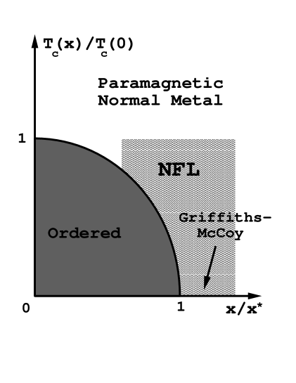
FIG. 1.: Typical phase diagram of the systems studied with an ordered magnetic phase and an anomalous metallic phase close to the QCP. The Griffiths-McCoy singularities appear close to the QCP.

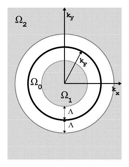
FIG. 2.: Fermi Surface and its regions of energy.

FIG. 3.: Plot of ${\cal F}(2x,y)$ which appears in the expression for the RKKY interaction (16): dashed line is the usual RKKY ($\Lambda=0$); continuous line $\Lambda/k_{F}=0.1$.

FIG. 4.: Plot of the first zero of the RKKY interaction, $y=k_{F}r_{0}$, as a function of $x=\Lambda/k_{F}$.

FIG. 5.: Percolation problem in a (a) Kondo hole system and (b) Ligand system. $\rho_{e}$ is the electronic density; $\rho_{f}$ is the density of magnetic moments; $\rho_{Q}$ is the density of compensated moments; $p$ is the percolation parameter and $p_{c}$ is the percolation threshold.

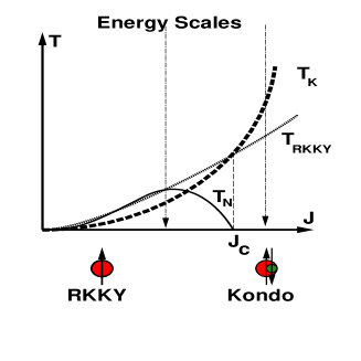
FIG. 6.: Doniach phase diagram: long dashed line is the Kondo temperature, $T_{K}$; short dashed line is the RKKY temperature,$T_{RKKY}$; the continuous line is the ordering temperature $T_{N}$.

FIG. 7.: Energy level splitting in the two-impurity Kondo effect.

FIG. 8.: Behavior of the scaling functions of the magnetization, $f_{\lambda}(H/T)$, given in (210) and the specific heat, $g_{\lambda}(H/T)$, given by (230), in the $H\times T$ phase diagram. The line $T\sim H$ marks the crossover in behavior and $\Gamma$ is the value of the RKKY interaction above which the cluster does not exist.

REFERENCES

- [1] G. R. Stewart, Rev. Mod. Phys. 56, 755 (1984); Z. Fisk, D. W. Hess, C. J. Pethick, D. Pines, J. L. Smith, J. D. Thompson and J. O. Willis, Science 239, 33 (1988); A. C. Hewson, The Kondo Problem to Heavy Fermions (Cambridge Press, New York, 1993).
- [2] J. A. Hertz, Phys. Rev. B 14, 1165 (1976).
- [3] S. Sachdev and J. W. Ye, Phys. Rev. Lett. 69, 2411 (1992); A. M. Tsvelik and M. Reizer, Phys. Rev. B 48, 9887 (1993); A. J. Millis, Phys. Rev. B 48, 7183 (1993); M. A. Continentino,Phys. Rep. 239, 179 (1994); L. B. Ioffe and A. J. Millis, Phys. Rev. B 51, 16151 (1995).
- [4] P. Nozières, Theory of Interacting Fermi Systems, (Benjamim, New York, 1964); A. A. Abrikosov, L. P. Gorkov and I. E. Dzyaloshinski, Methods of Quantum Field Theory in Statistical Physics, (Dover, New York, 1975); D. Pines and P. Nozières, Theory of Quantum Liquids, Vol. I, (Addison-Wesley, Redwood City, 1989); G. Baym and C. Pethick, Landau Fermi-Liquid Theory, (John Wiley, New York,1991).
- [5] G. D. Mahan, Many-Particle Physics, (Plenum Press, New York, 1990).
- [6] B. L. Altshuler and A. G. Aronov, Sol. State. Comm. 46, 429-435 (1983); A. M. Finkelstein, Z. Phys. B 56, 189-196 (1984); W. L. McMillan, Phys. Rev. B 31, 2750 (1985); C. Castellani and C. Di Castro, Phys. Rev. B 34, 5935 (1986); C. Castellani, G. Kotliar and P. A. Lee, Phys. Rev. Lett. 59, 322 (1987).
- [7] E. Abrahams, P. W. Anderson, D. C. Licciardello and T. V. Ramakrishnan, Phys. Rev. Lett. 42, 637 (1979).
- [8] For a review of the experimental situation see, for instance, the papers presented at the Conference on Non-Fermi liquid behavior in Metals, J. Phys. Cond. Mat 8, 1996.
- [9] M. C. Aronson, R. Osborn, R. A. Robinson, J. W. Lynn, R. Chau, C. L. Seaman and M. B. Maple, Phys. Rev. Lett. 75, 725 (1995).
- [10] C. H. Booth, D. E. MacLaughlin, R. H. Heffner, R. Chau, M. B. Maple and G. H. Kwei, Phys. Rev. Lett. 81, 3960 (1998).
- [11] O. O. Bernal, D. E. MacLaughlin, H. G. Lukefahr and A. Andraka, Phys. Rev. Lett. 75, 2023 (1995).
- [12] M. Lenkewitz, S. Corsépius, G. -F. v. Blanckenhagen and G. R. Stewart, Phys. Rev. B 55, 6409 (1997).
- [13] C. L. Seaman, M. B. Maple, B. W. Lee and S. Ghamaty, Phys. Rev. Let. 67, 2882 (1991).
- [14] J. L. Gavilano, J. Hunziker and H. R. Ott, Phys. Rev. B 52, 13106 (1995).
- [15] S. A. M. Mentink, G. J. Nieuwenhuys, A. A. Menovsky, J. A. Mydosh, H. Tou and Y. Kitaoka, Phys. Rev. B 49, 15759 (1994).
- [16] A brief review of the experimental and theoretical situation can be found in A. H. Castro Neto, Proceedings of the VI International Summer School “Nicolás Cabrera”, 1999 (cond-mat/9911092).
- [17] J. Kondo, Prog. Theoret. Phys. 32, 37 (1964); Solid State Physics, vol. 23, H. Ehrenreich, F. Seitz and D. Turnbull, eds., (Academic Press, New York, 1969), p. 183.
- [18] P. Coleman, Phys. Rev. B 29, 3035 (1984); T. M. Rice and K. Ueda, Phys. Rev. Lett. 55, 995 (1985); G. Kotliar and A. E. Ruckenstein, Phys. Rev. Lett. 57, 1362 (1986); N. E. Bickers,Rev. Mod. Phys. 59, 845 (1987); D. M. Newns and N. Read, Advances in Physics 36, 799 (1987); A. J. Millis and P. A. Lee, Phys. Rev. B 35, 3394 (1987).
- [19] P. Nozières and A. Blandin, J. Physique 41, 193 (1980).
- [20] D. L. Cox, Phys. Rev. Lett. 59, 1240 (1987).
- [21] E. Miranda, V. Dobrosavljević and G. Kotliar, Phys. Rev. Lett. 78, 290 (1997).
- [22] H. v. Löhneysen, T. Pietrus, G. Portisch, H. G. Schlager, A. Schröder, M. Sieck, and T. Trappmann, Phys. Rev. Lett. 72, 3262 (1994).
- [23] A. Schröder, G. Aeppli E. Bucher, R. Ramazashvili, and P. Coleman, Phys. Rev. Lett. 80, 5623 (1998); R. Ramazashvili, cond-mat/9901191.
- [24] O. Stockert, H. v. Löhneysen, A. Rosch, N. Pyka and M. Loewenhaupt, Phys. Rev. Lett. 80, 5627 (1998).
- [25] B. Andraka and A. M. Tsvelik, Phys. Rev. Lett. 67, 2886 (1991).
- [26] A. M. Sengupta and A. Georges, Phys. Rev. B 52, 10295, (1995).
- [27] J. A. Hertz, Phys. Rev. B 18, 4875 (1978).
- [28] R. N. Bhatt and D. Fisher, Phys. Rev. Lett. 68, 3072 (1992).
- [29] See, for instance, S. Sachdev, Phil. Trans. R. Soc., 356, 173 (1998) and references therein.
- [30] See, for instance, T. Vojta, cond-mat/9910514 and references therein.
- [31] S. Doniach, Physica B 91B, 231 (1977).
- [32] A. H. Castro Neto, G. E. Castilla and B. A. Jones, Phys. Rev. Lett. 81, 3531 (1998).
- [33] R. B. Griffiths, Phys. Rev. Lett. 23, 17 (1969).
- [34] B. M. McCoy and T. T. Wu, Phys. Rev. 176, 631 (1968); B. McCoy, Phys. Rev. B 2, 2795 (1970).
- [35] Ch. Binek, S. Kuttler and W. Kleemann, Phys. Rev. Lett. 75, 2412 (1995); H. Deguchi, M. Aikawa, K. Ohtani and S. Tagaki, Jour. Mag. Magn. Mat. 177, 87 (1998).
- [36] D. S. Fisher, Phys. Rev. B 51, 6411 (1995).
- [37] T. Senthil and S. Sachdev, Phys. Rev. Lett. 77, 5292 (1996).
- [38] M. Y. Guo, R. N. Bhatt and D. A. Huse, Phys. Rev. Lett. 72, 4137 (1994); H. Rieger and A. P. Young, Phys. Rev. Lett. 72, 41 41 (1994); C. Pich, A. P. Young, H. Rieger and N. Kawashima, Phys. Rev. Lett. 81, 5916 (1998); T. Ikegami, S. Miyashita and H. Rieger, Jour. Phys. Soc. Japan 67, 2671 (1998).
- [39] M. C. de Andrade, R. Chau, R. P. Dickey, N. R. Dilley, E. J. Freeman, D. A. Gajewski, M. B. Maple, R. Movshovich, A. H. Castro Neto, G. E. Castilla and B. A. Jones, Phys. Rev. Lett. 81, 5620-5623 (1998).
- [40] P. W. Anderson, Phys. Rev. 124, 41 (1961).
- [41] A. H. Castro Neto and B. A. Jones, unpublished.
- [42] M. A. Rudermann and C. Kittel, Phys. Rev. 96, 99 (1954); T. Kasuya, Prog. Theo. Phys. (Kyoto) 16, 45 (1956); K. Yosida, Phys. Rev. 106, 893 (1957).
- [43] This kind of approach has been proposed in the context of the two impurity problem by V. Barzykin and I. Affleck, cond-mat/9909186.
- [44] E. Fradkin, Field Theories of Condensed Matter Systems, (Addison-Wesley, Redwood City, 1991).
- [45] See, for instance, J. R. Iglesias, C. Lacroix and B. Coqblin, Phys. Rev. B 56, 11820 (1997).
- [46] L. M. Roth, H. J. Zeiger and T. A. Kaplan, Phys. Rev. 149, 519 (1966).
- [47] P. G. de Gennes, J. Phys. Radium 23, 630 (1962).
- [48] I. Dzyaloshinsky, J. Phys. Chem. Solids 4, 241 (1958); T. Moriya,Phys. Rev. 120, 91 (1960).
- [49] See, for instance, K. Yosida, Theory of Magnetism (Springer, Berlin, 1991) and references therein.
- [50] W. C. Koeler, Phys. Rev. 118, 58 (1960).
- [51] E. M. Lifshitz, Zh. Eksp. Teor. Fiz. 11, 253 (1941); ibid., 11, 269 (1941).
- [52] D. C. Mattis, Theory of Magnetism, (Harper and Row, New York, 1965).
- [53] A. Jagannathan, E. Abrahams and M. J. Stephen, Phys. Rev. B 37,436 (1988).
- [54] V. Jaccarino and L. R. Walker, Phys. Rev. Lett. 15, 258 (1965).
- [55] For a review see, for instance, the papers published in Magnetism in Alloys, P. A. Bech and J. T. Waber, eds. (New York, MEall. Sco. AIME, 1972).
- [56] A. I. Larkin and V. I. Mel’nikov, Sov. Phys. JETP 34, 656 (1972).
- [57] C. Jayaprakash, H. R. Krishnamurthy and J. W. Wilkins, Phys. Rev. Lett. 47, 737 (1981); B. A. Jones and C. M. Varma, Phys. Rev. Lett. 58, 843 (1987); B. A. Jones, C. M. Varma and J. W. Wilkins, Phys. Rev. Lett. 61, 125 (1988); B. A. Jones and C. M. Varma, Phys. Rev. B 40, 324 (1989); A. J. Millis, G. Kotliar, and B. A. Jones, in Field Theories in Condensed Matter Physics, Z. Tesanovic, ed. (Addison-Wesley, Redwood City, 1990).
- [58] P. Nozières, Ann. Phys. (Paris) 10, 19 (1985).
- [59] S. R. Garner, Y. W. Rodriguez, Z. Schlesinger, B. Bucher, Z. Fisk and J. L. Sarrao, cond-mat/9910485.
- [60] D. Stauffer, Introduction to Percolation Theory (Taylor & Francis, London, 1985).
- [61] A. J. Leggett, S. Chakravarty, A. T. Dorsey, Matthew P. A. Fisher, Anupam Garg and W. Zwerger, Rev. Mod. Phys. 59, 1 (1987); V. J. Emery and S. A. Kivelson, in Fundamental Problems in Statistical Mechanics, VIII, H. van Beijeren and M. H. Ernst, eds. (Elsevier, Amsterdam, 1994); G. Kotliar and Q. Si, Phys. Rev. B 53, 12373 (1996).
- [62] P. W. Anderson, G. Yuval and D. R. Hamann, Phys. Rev. B 1, 4464 (1970).
- [63] F. Lesage and H. Saleur, Phys. Rev. Lett. 80, 4370 (1998).
- [64] T. A. Costi and G. Zarand, Phys. Rev. B 59, 12398 (1999).
- [65] H. Saleur, unpublished.
- [66] J. W. Gan, Phys. Rev. B 51, 8287 (1995); I. Affleck, A. W. W. Ludwig and B. A. Jones, Phys. Rev. B 52, 9528 (1995).
- [67] P. C. E. Stamp, E. M. Chudnovsky and B. Barbara, Int. Jour. Mod. Phys. B 6, 1355 (1992).
- [68] N. V. Prokof’ev and P. C. E. Stamp, J. Low Temp. Phys. 104, 143 (1996).
- [69] For a review on the problem of tunneling of magnetization, see, for instance, E. M. Chudnovsky and J. Tejada, Macroscopic Quantum Tunneling of the Magnetic Moment, (Cambridge University Press, 1998) and references therein.
- [70] L. D. Landau and E. M. Lifshitz, Sov. Phys. JETP 8, 153 (1935); T. L. Gilbert, Phys. Rev. 100, 1243 (1955).
- [71] D. Loss, D. P. DiVincenzo and G. Grinstein, Phys. Rev. Lett. 69, 3232 (1992); J. von Delft and C. L. Henley, Phys. Rev. Lett. 69, 3236 (1992).
- [72] M. J. Thill and D. A. Huse, Physica A 214, 321 (1995).
- [73] R. A. Fisher, S. E. Lacy, C. Marcenat, J. A. Olsen, N. E. Phillips, J. Flouquet, A. Amato and D. Jaccard, Jap. Journ. Appl. Phys. 26, 1257 (1987).
- [74] J. S. Kim and G. R. Stewart, Phys. Rev. B 49, 327 (1994).
- [75] R. Vollmer, T. Pietrus, H. v. Löhneysen, R. Chau and M. B. Maple, Phys. Rev. B 61, 1218 (2000).
- [76] H. Rieger and F. Iglói, Phys. Rev. Lett. 83, 3741 (1999).