Moment free energies for polydisperse systems

Abstract

A polydisperse system contains particles with at least one attribute $\sigma$ (such as particle size in colloids or chain length in polymers) which takes values in a continuous range. It therefore has an infinite number of conserved densities, described by a density distribution $\rho(\sigma)$. The free energy depends on all details of $\rho(\sigma)$, making the analysis of phase equilibria in such systems intractable. However, in many (especially mean-field) models the excess free energy only depends on a finite number of (generalized) moments of $\rho(\sigma)$; we call these models truncatable. We show, for these models, how to derive approximate expressions for the total free energy which only depend on such moment densities. Our treatment unifies and explores in detail two recent separate proposals by the authors for the construction of such moment free energies. We show that even though the moment free energy only depends on a finite number of density variables, it gives the same spinodals and critical points as the original free energy and also correctly locates the onset of phase coexistence. Results from the moment free energy for the coexistence of two or more phases occupying comparable volumes are only approximate, but can be refined arbitrarily by retaining additional moment densities. Applications to Flory-Huggins theory for length-polydisperse homopolymers, and for chemically polydisperse copolymers, show that the moment free energy approach is computationally robust and gives new geometrical insights into the thermodynamics of polydispersity.

I Introduction

The thermodynamics of mixtures of several chemical species is, since Gibbs, a well established subject (see e.g. [1]). But many systems arising in nature and in industry contain, for practical purposes, an infinite number of distinct, though similar, chemical species. Often these can be classified by a parameter, $\sigma$, say, which could be the chain length in a polymeric system, or the particle size in a colloid; both are routinely treated as continuous variables. In other cases (see e.g. [2, 3, 4, 5]) $\sigma$ is instead a parameter distinguishing species of continuously varying chemical properties. In the most general case, several attributes may be required to distinguish the various particle species in the system (such as length and chemical composition in length-polydisperse random copolymers) and $\sigma$ is then a collection of parameters [6]. The thermodynamics of polydisperse systems (as defined above) is of crucial interest to wide areas of science and technology; it is sometimes also referred to as “continuous thermodynamics” (see e.g. [3]).

Standard thermodynamic procedures [1] for constructing phase equilibria in a system of volume $V$ containing $M$ different species can be understood geometrically in terms of a free energy surface $f(\rho_{j})$ (with $f=F/V$, and $F$ the Helmoltz free energy) in the $M$-dimensional space of number densities $\rho_{j}$. Tangent planes to $f$ define regions of coexistence, within which the free energy of the system is lowered by phase separation. The volumes of coexisting phases follow from the well-known “lever rule”[1]. Here “surface” and “plane” are used loosely, to denote manifolds of appropriate dimension. This procedure becomes unmanageable, both conceptually and numerically, in the limit $M\to\infty$ which formally defines a polydisperse system. There is now a separate conserved density $\rho(\sigma)$ for each value of $\sigma$; $\rho(\sigma)$ is in fact a density distribution and the overall number density of particles is written as $\rho=\int\!d\sigma\,\rho(\sigma)$. The free energy surface is $f=f[\rho(\sigma)]$ (a functional) which resides in an infinite-dimensional space. Gibbs’ rule allows the coexistence of arbitrarily many thermodynamic phases.

To make phase equilibria in polydisperse systems more accessible to both computation and physical intuition, it is clearly helpful to reduce the dimensionality of the problem. Theoretical work in this area has made significant progress in finding simplified forms of the conditions for phase coexistence, thus making these more numerically tractable [3, 4, 5, 7, 8, 9, 10, 11, 12, 13, 14, 15, 16, 17]. Our aim is to achieve a similar reduction in dimensionality on a higher level, that of the free energy itself. We show that, for a large class of models, it is possible to construct a reduced free energy depending on only a small number of variables. From this, meaningful information on phase equilibria can be extracted by the usual tangent plane procedure, with obvious benefits for a more intuitive understanding of the phase behavior of polydisperse systems. As an important side effect, this procedure also leads to robust algorithms for calculating polydisperse phase equilibria numerically. In particular, such algorithms can handle coexistence of more than two phases with relative ease compared to those used previously[7, 13, 15, 16, 18, 19, 20, 21, 22, 23, 24, 25].

A clue to the choice of independent variables for such a reduced free energy comes from the representation of experimental data. We recall first the definition of a “cloud point” (see e.g. [3, 7, 26]): This is the point at which, for a system with a given density distribution $\rho(\sigma)$, phase separation first occurs as the temperature $T$ or another external control parameter is varied. The corresponding incipient phase is called the “shadow”. Now consider diluting or concentrating the system, i.e., varying its overall density $\rho$ while maintaining a fixed “shape” of polydispersity $n(\sigma)=\rho(\sigma)/\rho$. We will find it useful later to refer to the collection of all systems $\rho(\sigma)=\rho n(\sigma)$ which can be obtained by this process as a “dilution line” (in the space of all density distributions $\rho(\sigma)$). Plotting the cloud point temperature $T$ versus density $\rho$ then defines the cloud point curve (CPC), while plotting $T$ versus the density of the shadow gives the shadow curve [27]. The differences in the shapes $n(\sigma)$ of the density distributions in the different phases are hidden in this representation; only the overall densities $\rho$ in each phase are tracked. The density $\rho$ is a particular moment of $\rho(\sigma)$ (the zeroth one); higher order moments would be given by $\int\!d\sigma\,\sigma^{i}\rho(\sigma)$. Generalizing slightly, this suggests that our reduced free energy should depend on several (generalized) moment densities $\rho_{i}=\int\!d\sigma\,w_{i}(\sigma)\rho(\sigma)$, defined by appropriate (linearly independent) weight functions $w_{i}(\sigma)$. Ordinary power-law moment densities are included as the special case $w_{i}(\sigma)=\sigma^{i}$. Whatever the choice of moments, we insist on $w_{0}=1$ so that in all cases the zeroth moment density $\rho_{0}$ coincides with the overall number density $\rho$.

As an illustration, consider the simplest imaginable case where the true free energy $f$ already has the required form, i.e., it depends only on a finite set of $K$ moment densities of the density distribution:

$$f=f(\rho_{i}),\qquad i=1\ldots K\quad{\mathrm{o}r}\quad i=0\ldots K-1$$ (1)

where the range of $i$ depends on whether $\rho_{0}\equiv\rho$ is among the $K$ moment densities on which $f$ depends. (From now on, we use the notation $i=1\ldots K$ inclusively, to cover both possibilities.) In coexisting phases one demands equality of particle chemical potentials, defined as $\mu(\sigma)={\delta f/\delta\rho(\sigma)}$, for all $\sigma$. Because

$\displaystyle\mu(\sigma)\equiv\frac{\delta f}{\delta\rho(\sigma)}=\sum_{i}\frac{\partial f}{\partial\rho_{i}}w_{i}(\sigma)=\sum_{i}\mu_{i}w_{i}(\sigma)$

this implies that all “moment” chemical potentials, $\mu_{i}\equiv{\partial f}/{\partial\rho_{i}}$, are likewise equal among phases. The second requirement for phase coexistence is that the pressures or osmotic pressures [28], $\Pi$, of all phases must also be equal. But from

$\displaystyle-\Pi=f-\int\!d\sigma\,\mu(\sigma)\rho(\sigma)=f-\sum_{i}\mu_{i}\rho_{i}$

one sees that this again involves only the moment densities $\rho_{i}$ and their chemical potentials $\mu_{i}$. Finally, the moment densities also obey the “lever rule”, as follows. Let the overall density distribution of a system of volume $V$ be $\rho^{(0)}(\sigma)$; we call this the “parent” distribution. If (after a lowering of temperature, for example) this parent has split into $p$ coexisting “daughter” phases with $\sigma$-distributions $\rho^{(\alpha)}(\sigma)$, each occupying a fraction $v^{(\alpha)}$ of the total volume ($\alpha=1\ldots p$), then particle conservation implies the usual lever rule (or material balance) among species: $\sum_{\alpha}v^{(\alpha)}\rho^{(\alpha)}(\sigma)=\rho^{(0)}(\sigma),\forall\sigma$. Multiplying this by a weight function $w_{i}(\sigma)$ and integrating over $\sigma$ shows that the lever rule also holds for the moment densities:

$$\sum_{\alpha=1}^{p}v^{(\alpha)}\rho_{i}^{(\alpha)}=\rho_{i}^{(0)}$$ (2)

These results express the fact that any linear combination of conserved densities (a generalized moment density) is itself a conserved density in thermodynamics. We have shown, therefore, that if the free energy of the system depends only on $K$ moment densities $\rho_{1}\ldots\rho_{K}$ we can view these as the densities of $K$ “quasi-species” of particles, and construct the phase diagram via the usual construction of tangencies and the lever rule. Formally this has reduced the problem to finite dimensionality, although this is trivial here because $f$, by assumption, has no dependence on any variables other than the $\rho_{i}$ ($i=1\ldots K$).

Of course, it is uncommon for the free energy $f$ to obey (1). In particular, the entropy of an ideal mixture (or, for polymers, the Flory-Huggins entropy term) is definitely not of this form. On the other hand, in very many thermodynamic (especially mean field) models the excess (i.e., non-ideal) part of the free energy does have the simple form (1). In other words, if we decompose the free energy as (setting $k_{\rm B}=1$)

$$f=-Ts_{\rm id}+\tilde{f},\quad s_{\rm id}=-\int\!d\sigma\,\rho(\sigma)\left[\ln\rho(\sigma)-1\right]$$ (3)

then the excess free energy $\tilde{f}$ is a function of some moment densities only:

$$\tilde{f}=\tilde{f}(\rho_{i}),\qquad i=1\ldots K$$ (4)

Examples of models of this kind include polydisperse hard spheres (within the generalization by Salacuse and Stell [8] of the BMCSL equation of state [29, 30]), polydisperse homo- and copolymers [2, 3, 4, 5, 9], and van der Waals fluids with factorized interaction parameters [10]. With the exception of a brief discussion in Sec. VI, this paper concerns models with free energies of the form (3,4), which we call “truncatable”. (This terminology emphasizes that the number $K$ of moment densities appearing in the excess free energy of truncatable models is finite, while for a non-truncatable model the excess free energy depends on all details of $\rho(\sigma)$, corresponding to an infinite number of moment densities.) In what follows, we regard each model free energy as given, and do not discuss the issue of how good a description of the real system it offers, nor how or whether it can be derived from an underlying microscopic Hamiltonian. Whenever we refer to “exact” results, we mean the exact thermodynamics of such a model as specified by its free energy.

Different authors refer in different terms to $s_{\rm id}$ in (3). Throughout this paper will call the quantity

$\displaystyle s_{\rm id}=-\int\!d\sigma\,\rho(\sigma)\left[\ln\rho(\sigma)-1\right]$

(which is, up to a factor of $-T$, the ideal part of the free energy density) the “entropy of an ideal mixture”. By writing $\rho(\sigma)=\rho n(\sigma)$, where $n(\sigma)$ is the normalized distribution of $\sigma$, this can be decomposed as

$$s_{\rm id}=-\rho(\ln\rho-1)-\rho\int\!d\sigma\,n(\sigma)\ln n(\sigma)$$ (5)

The first term on the right hand side is the “entropy of an ideal gas”, while the second term gives the “entropy of mixing”. The prefactor $\rho$ reflects the fact that both are expressed per unit volume rather than per particle.

In principle, the entire phase equilibria for any truncatable system (obeying (4)) can be computed exactly by a finite algorithm. Specifically, the spinodal stability criterion involves a $K$-dimensional square matrix [11, 12, 13, 14] whereas calculation of $p$-phase equilibrium involves solution of $(p-1)(K+1)$ coupled nonlinear equations (see Sec. III E). This method has certainly proved useful [2, 3, 4, 9, 10, 14], but is cumbersome, particularly if one is interested mainly in cloud- and shadow-curves, rather than coexisting compositions deep within multi-phase regions [2, 4, 9, 26]. Various ways of simplifying the procedure exist [7, 11, 15, 16, 17], but there has previously not been a systematic alternative to the full computation. Note also that the nonlinear phase equilibrium equations permit no simple geometrical interpretation or qualitative insight akin to the familiar rules for constructing phase diagrams from the free energy surface of a finite mixture. This further motivates the search for a description of polydisperse phase equilibria in terms of a reduced free energy which depends on only a small number of density variables.

In previous work, the authors originally arrived independently at two definitions of a reduced free energy in terms of moment densities (moment free energy for short) [31, 32]. Though based on distinctly different principles, the two approaches led to very similar results. We explain this somewhat surprising fact in the present work; at the same time, we describe the two methods in more detail and explore the relationship between them. We also discuss issues related to practical applications and give a number of example results for simple model systems.

The first route to a moment free energy takes as its starting point the conventional form of the ideal part of the free energy, $f_{\rm id}=T\int\!d\sigma\,\rho(\sigma)[\ln\rho(\sigma)-1]$, as in (3). This can be thought as defining a (hyper-)surface, with the “horizontal” co-ordinate being $\rho(\sigma)$ and the “height” of the surface $f_{\rm id}[\rho(\sigma)]$. As explained in Sec. II A, this surface can then be projected geometrically onto one with only a finite set of horizontal co-ordinates: these are chosen to be the moment densities appearing in the excess free energy. Physically, this corresponds to minimizing the free energy with respect to all degrees of freedom in $\rho(\sigma)$ that do not affect these moment densities. We call this first route the “projection” method.

The second approach rederives the entropy of mixing in the ideal part of the free energy in a form that depends explicitly only on the chosen moment densities. As described in Sec. II B, the expression that results is intractable in general because it still contains the full complexity of the problem. However, in situations where there are only infinitesimal amounts of all but one of the phases in the systems, the entropy of mixing can be evaluated in a closed form. Applying this functional form in regimes where it is not strictly valid (i.e., when phases of comparable volumes coexist) generates a moment free energy by this “combinatorial” method.

We show the equivalence of the two approaches in Sec. II C. There, we first demonstrate that the general form of the entropy of mixing obtained by the combinatorial method can be transformed to the standard expression $-\int\!d\sigma\,n(\sigma)\ln n(\sigma)$. Second, we show that the moment free energies arrived at by the two methods are in fact equal, with the projection method being slightly more generally applicable.

In Sec. III, we then discuss the properties of the moment free energy (as obtained from either the projection or the combinatorial method). By construction, it depends only on a (finite) number of moment densities, and so achieves the desired reduction in dimensionality. The moment densities can be treated as densities of “quasi-species” of particles, and the standard procedures of the thermodynamics of finite mixtures can be applied to the moment free energy to calculate phase equilibria. This is only useful, however, if the results are faithful to the actual phase behavior of the underlying polydisperse system (as modeled by the given truncatable free energy). We show that this is so: In fact, the construction of our moment free energy is such that exact binodals (cloud-point and shadow curves), critical (and multi-critical) points and spinodals are obtained. Beyond the onset of phase separation, where coexisting phases occupy comparable volumes, the results are not exact, but can be refined arbitrarily by adding extra moment densities. This procedure is necessary also to ensure that, in regions of multi-phase coexistence, the correct number of phases is found. In Sec. IV, we discuss the practical implementation of our method, followed by a number of examples (Sec. V). Our results are summarized in Sec. VI, where we also outline perspectives for future work.

Note that throughout this work, we focus on the case of phase coexistence at fixed volume. However, as described in App. A, the formalism can easily be applied to scenarios where the (mechanical or osmotic) pressure is fixed instead.

II Derivation of moment free energy

A Projection method

The starting point for this method is the decomposition (3) for the free energy of truncatable systems (4):

$$f=T\int\!d\sigma\,\rho(\sigma)\left[\ln\frac{\rho(\sigma)}{R(\sigma)}-1\right]+\tilde{f}(\rho_{i})$$ (6)

As explained in the previous section, truncatable here means that the excess free energy $\tilde{f}$ depends only on $K$ moment densities $\rho_{i}$. Note that, in the first (ideal) term of (6), we have included a dimensional factor $R(\sigma)$ inside the logarithm. This is equivalent to subtracting $T\int\!d\sigma\,\rho(\sigma)\ln R(\sigma)$ from the free energy. Since this term is linear in densities, it has no effect on the exact thermodynamics; it contributes harmless additive constants to the chemical potentials $\mu(\sigma)$. However, in the projection route to a moment free energy, it will play a central role.

We now argue that the most important moment densities to treat correctly are those that actually appear in the excess free energy $\tilde{f}(\rho_{i})$. Accordingly we divide the infinite-dimensional space of density distributions into two complementary subspaces: a “moment subspace”, which contains all the degrees of freedom of $\rho(\sigma)$ that contribute to the moment densities $\rho_{i}$, and a “transverse subspace” which contains all remaining degrees of freedom (those that can be varied without affecting the chosen moment densities $\rho_{i}$) [33]. Physically, it is reasonable to expect that these “leftover” degrees of freedom play a subsidiary role in the phase equilibria of the system, a view justified a posteriori below. Accordingly, we now allow violations of the lever rule, so long as these occur solely in the transverse space. This means that the phase splits that we calculate using this approach obey the lever rule for the moment densities, but are allowed to violate it in other details of the density distribution $\rho(\sigma)$ (see Fig. 10 in Sec. V B 1 for an example). These “transverse” degrees of freedom, instead of obeying the strict particle conservation laws, are chosen so as to minimize the free energy: they are treated as “annealed”. If, as assumed above, $\tilde{f}=\tilde{f}(\rho_{i})$ only depends on the moment densities retained, this amounts to maximizing the ideal mixture entropy ($s_{\rm id}$) in (6), while holding fixed the values of the moment densities $\rho_{i}$. Note that we are allowed, if we wish, to include among the retained densities “redundant” moments on which $\tilde{f}$ has a null dependence. We will have occasion to do this later on.

At this point, the factor $R(\sigma)$ in (6), which is immaterial if all conservation laws are strictly obeyed, becomes central. Indeed, maximizing the entropy over all distributions $\rho(\sigma)$ at fixed moment densities $\rho_{i}$ yields

$$\rho(\sigma)=R(\sigma)\exp\left(\sum_{i}\lambda_{i}w_{i}(\sigma)\right)$$ (7)

where the Lagrange multipliers $\lambda_{i}$ are chosen to give the desired moment densities

$$\rho_{i}=\int\!d\sigma\,w_{i}(\sigma)\,R(\sigma)\exp\left(\sum_{i}\lambda_{i}w_{i}(\sigma)\right)$$ (8)

The corresponding minimum value of $f$ then defines our projected free energy as a function of the moment densities $\rho_{i}$:

$$f_{\rm pr}(\rho_{i})=-Ts_{\rm pr}(\rho_{i})+\tilde{f}(\rho_{i}),\qquad s_{\rm pr}=\rho_{0}-\sum_{i}\lambda_{i}\rho_{i}$$ (9)

Here $s_{\rm pr}$ is the projected entropy of an ideal mixture. The first term appearing in it, $\rho_{0}=\int\!d\sigma\,\rho(\sigma)$, is the “zeroth moment”, which is identical to the overall particle density $\rho$ defined previously. If this is among the moment densities used for the projection (or more generally, if it is a linear combination of them), then the term $-T\rho_{0}$ is simply a linear contribution to the projected free energy $f_{\rm pr}(\rho_{i})$ and can be dropped because it does not affect phase equilibrium calculations. Otherwise, $\rho_{0}$ needs to be expressed – via the $\lambda_{i}$ – as a function of the $\rho_{i}$ and its contribution cannot be ignored. We will see an example of this in Sec. V.

The projection method yields a free energy $f_{\rm pr}(\rho_{i})$ which only depends on the chosen set of moment densities. These can now be viewed as densities of ‘quasi-species’ of particles, and a finite-dimensional phase diagram can be constructed from $f_{\rm pr}$ according to the usual rules, ignoring the underlying polydisperse nature of the system. Obviously, though, the results now depend on $R(\sigma)$ which is formally a “prior distribution” for the entropy maximization. To understand its role, we recall that the projected free energy $f_{\rm pr}(\rho_{i})$ was constructed as the minimum of $f[\rho(\sigma)]$ at fixed $\rho_{i}$; that is, $f_{\rm pr}$ is the lower envelope of the projection of $f$ onto the moment subspace. Crucially, the shape of this envelope depends on how, by choosing a particular prior distribution $R(\sigma)$, we “tilt” the infinite-dimensional free energy surface before projecting it. This geometrical point of view is illustrated, for a mixture of only two species, in Fig. 1.

FIG. 1.: Illustration of free energy projection. The full infinite-dimensional free energy surface $f[\rho(\sigma)]$ for a truly polydisperse system cannot be represented graphically, so a system with only two particle species is used instead. A single phase is then described by its density pair $(r_{1},r_{2})$. (The projection method remains applicable, although the polydispersity parameter $\sigma$ is replaced by a discrete species index $a\in\{1,2\}$, and integrals $\int\!d\sigma\,\rho(\sigma)\ldots$ by $\sum_{a}r_{a}\ldots$) To illustrate the method we choose a model with an excess free energy depending on a single moment density $\rho_{1}=L_{1}r_{1}+L_{2}r_{2}$ (in fact Flory-Huggins theory for length polydispersity, discussed in more detail in Sec. V; see (70)). Both the transverse and the moment subspace are then one-dimensional. (a) 3d-view of free energy surface. The circle marks the position of the parent ($r^{(0)}_{1},r^{(0)}_{2}$); the thick line traces out the free energy of density pairs ($r_{1},r_{2}$) in the corresponding family (10). (b) Top view, showing as dashed lines the transverse directions along which the moment density $\rho_{1}$ is constant. (c) Side view of the free energy surface, “looking down” the transverse direction. (d) The projected free energy is simply the lower envelope of the free energy surface as seen from this transverse direction. (e-h) The same free energy surface, now tilted differently by using a different parent (or prior). While this does not affect the location of any double tangent planes drawn to the full surface, it does produce a different “lower envelope” and hence a different projected free energy. For continuum polydispersity, the role of the density pair $(r_{1},r_{2})$ is played by a density distribution $\rho(\sigma)$ of a continuous parameter $\sigma$.

To understand the effect of the prior $R(\sigma)$ physically, we note that the projected free energy is simply the free energy of phases of a system in which the density distributions $\rho(\sigma)$ are of the form (7). The prior $R(\sigma)$ determines which distributions lie within this “maximum entropy family” (or “family” for short), and it is the properties of phases with these distributions that the projected free energy represents. Typically, one is interested in a system where a fixed overall “parent” (or “feed”) distribution $\rho^{(0)}(\sigma)$ becomes subject to separation into various phases. In such circumstances, we should generally choose this parent distribution as our prior, $R(\sigma)=\rho^{(0)}(\sigma)$, thereby guaranteeing that it is contained within the family (7). Having done this, we note that the projection procedure will be exactly valid, to whatever extent the density distributions actually arising in the various coexisting phases of the system under study are members of the corresponding family

$$\rho(\sigma)=\rho^{(0)}(\sigma)\exp\left(\sum_{i}\lambda_{i}w_{i}(\sigma)\right).$$ (10)

In fact, the condition just described holds whenever all but one of a set of coexisting phases are of infinitesimal volume compared to the majority phase. This is because the density distribution, $\rho^{(0)}(\sigma)$, of the majority phase is negligibly perturbed, whereas that in each minority phase differs from this by a Gibbs-Boltzmann factor, of exactly the form required for (10); we show this formally in Sec. III. Accordingly, our projection method yields exact cloud point and shadow curves. By the same argument, critical points (which in fact lie at the intersection of these two curves) are exactly determined; the same is true for tricritical and higher order critical points. Finally, spinodals are also found exactly. We defer explicit proofs of these statements to Sec. III.

The projection method does, however, give only approximate results for coexistences involving finite amounts of different phases. This is because linear combinations of different density distributions from the family (10), corresponding to two (or more) phases arising from the same parent $\rho^{(0)}(\sigma)$, do not necessarily add to recover the parent distribution itself:

$$\sum_{\alpha}v^{(\alpha)}\rho^{(0)}(\sigma)\exp\left(\sum_{i}\lambda_{i}^{(\alpha)}w_{i}(\sigma)\right)\neq\rho^{(0)}(\sigma)$$ (11)

unless all except one of the $v^{(\alpha)}$ are infinitesimal. Moreover, according to Gibbs’ phase rule, a projected free energy depending on $n$ moment densities will not normally predict more than $n+1$ coexisting phases, whereas a polydisperse system can in principle separate into an arbitrary number of phases. We explain in Sec. III how both of these shortcomings can be overcome by systematically including extra moment densities within the projection procedure. How quickly convergence to the exact results occurs depends on the choice of weight functions for the extra moment densities; we discuss this point further in the context of the examples of Sec. V.

B Combinatorial method

Now we turn to the second method of constructing a moment free energy. As before, we recognize from the outset that the physics of the problem is contained in the excess free energy and therefore the most important variables are the moment densities which feature in this. On the other hand, the ideal part of the free energy (essentially the entropy of mixing, up to the trivial ideal gas term) is a book-keeping device that accounts for the number of ways of partitioning a priori a given size distribution between two or more coexisting phases. (To focus the discussion, we identify $\sigma$ as particle size in this section; the arguments do of course remain valid for a general polydispersity parameter $\sigma$.) The entropy of mixing has its origin in $1/N!$ factors in the partition function (where $N$ is a particle number) which are usually derived from the classical limit of quantum statistics. The origin of the $1/N!$ factors in classical statistical mechanics has been the subject of debate ever since Gibbs [34]. The problem is also connected with the question of the extensivity of entropy, and the Gibbs paradox. Below we present a completely classical derivation of the entropy of mixing which has the additional benefit of indicating the appropriate generalisation for moment densities. To start with, follow Gibbs and define a non-extensive free energy $F^{\prime}$ as a configuration space ($\Gamma$) integral

$$e^{-F^{\prime}/T}=\int d\Gamma\,e^{-H/T}.$$ (12)

No $1/N!$ appears in this as all particles are distinguishable in classical statistical mechanics.

Now consider two phases in coexistence as one joint system. Assume they occupy volumes $V^{(1)}$ and $V^{(2)}$, respectively, and contain $N^{(1)}$ and $N^{(2)}$ particles. Following literally the prescription in eq. (12), the free energy of the joint system of $N^{(1)}+N^{(2)}=N$ particles is found from

$$e^{-F^{\prime}/T}=\sum_{\mathrm{prtns}}e^{-({F^{\prime}}^{(1)}+{F^{\prime}}^{(2)})/T}$$ (13)

where the configuration space integral has been done in two parts. Firstly, for each way of partitioning the particles between the two phases, the individual configuration space integrals give a product of the individual partition functions. Secondly, and crucially, one must sum over the $N!/N^{(1)}!N^{(2)}!$ ways of partitioning the particles between phases. Now define an extensive free energy by reinserting the $1/N!$ as though the particles were indistinguishable:

$$e^{-F_{\rm in}/T}=\frac{1}{N!}\int d\Gamma\,e^{-H/T},$$ (14)

Eq. (13) can then be written as

$$e^{-F_{\rm in}/T}=\langle e^{-(F_{\rm in}^{(1)}+F_{\rm in}^{(2)})/T}\rangle_{\mathrm{prtns}}$$ (15)

where the average is taken over all partitions, with equal a priori probabilities. This result is the cornerstone of the combinatorial method. If we separate $F_{\rm in}$ into the entropy of an ideal gas and the remaining non-ideal (excess) parts, it is written as

$$F_{\rm in}=NT[\ln(N/V)-1]+\tilde{F}$$ (16)

with $\tilde{F}$ being the excess free energy. Note that $F_{\rm in}$ does not yet contain an entropy of mixing term because it treats the particles as though they are indistinguishable. The entropy of mixing will reappear when we come to do the average over partitions in (15). Note also that conventional thermodynamics follows from (15) if all particles are identical as far as their mutual interactions are concerned. There is then no entropy of mixing to consider, so that $F_{\rm in}$ is just the conventional free energy $F$; and since the average over partitions is trivial one has $F=F^{(1)}+F^{(2)}$. Similarly, as we show in Sec. II C, one can recover from (15) the conventional form of the entropy of mixing as given in (5).

We now show how the average over partitions in (15) results in an expression for the entropy of mixing which depends explicitly on moment variables. The key is to note that, by our assumption that we are dealing with a truncatable model, the excess free energy $\tilde{F}=V\tilde{f}(\rho_{i})$ depends only on a limited number of moment densities $\rho_{i}$ (as well as volume $V$, temperature $T$, and other state variables which we suppress below). If the density $\rho_{0}$ is among the moment densities $\rho_{i}$ – which we assume throughout this section – then specifying $V$ and the $\rho_{i}$ is equivalent to specifying $N$, $V$ and the normalized moments $m_{i}=\rho_{i}/\rho_{0}$ ($i>0$). So we can think of $\tilde{F}$ as a function of $N$, $V$ and the $m_{i}$. From (16), $F_{\rm in}$ then depends on the same set of variables. The choice of the $m_{i}$, which are moments of the normalized particle size distribution $n(\sigma)$, as independent variables is natural in the present context because we are considering the particle number $N$ and volume $V$ of the coexisting phases to be fixed.

To avoid notational complexity, and without loss of generality, we now specialize to the case where there is only one normalized moment $m_{i}$, a generalized mean size

$\displaystyle m=\int\!d\sigma\,w(\sigma)n(\sigma)$

We shall also write $\rho_{m}=\rho m=\int\!d\sigma\,w(\sigma)\rho(\sigma)$ for the corresponding moment density, and $m^{(1)}$ and $m^{(2)}$ for the values of the generalized mean size in the first and second phase. The overall (“parent”) size distribution is $n^{(0)}(\sigma)$ with mean $m^{(0)}$. In each of the two phases, in which $N$ and $V$ are held fixed, $F_{\rm in}$ only depends on $m$, and so the average over partitions becomes

$$\langle e^{-(F_{\rm in}^{(1)}+F_{\rm in}^{(2)})/T}\rangle_{\mathrm{prtns}}\to\int dm^{(1)}\,{\cal P}(m^{(1)})\,e^{-(F_{\rm in}^{(1)}+F_{\rm in}^{(2)})/T}$$ (17)

Here ${\cal P}(m^{(1)})$ is the probability distribution for the generalized mean size in the first phase, taken over partitions with fixed $N^{(1)}$ and $N^{(2)}$, with equal a priori probabilities. Note that given $m^{(1)}$, $m^{(2)}$ is fixed in the second phase by the moment equivalent of particle conservation: $N^{(1)}m^{(1)}+N^{(2)}m^{(2)}=Nm^{(0)}$. The integral in (17) can be replaced by the maximum of the integrand in the thermodynamic limit, because $\ln{\cal P}(m^{(1)})$ is an extensive quantity. Introducing a Lagrange multiplier $\mu_{m}$ for the above moment constraint then shows that the quantity $\rho_{m}$ has the same status as the density $\rho\equiv\rho_{0}$ itself: both are thermodynamic density variables. This reinforces the discussion in the introduction, where we showed that moment densities can be regarded as densities of “quasi-species” of particles.

In what follows, we only need to refer to $m^{(1)}$ (not $m^{(2)}$) and therefore drop the superscript for brevity. Since $\ln{\cal P}(m)$ is extensive, we can write $\ln{\cal P}(m)=Ns(m)$ where $s$ is the entropy of mixing per particle expressed as a function of the moment $m$ (or, more generally, of the full set of normalized moments). The total free energy of the system then takes the form

$$F_{\rm in}=\min_{m}F_{\rm in}^{(1)}+F_{\rm in}^{(2)}-NTs(m),$$ (18)

and we need to calculate the entropy of mixing $s(m)$. We recognize that this quantity depends not only on the generalized mean size, but also on $x=N^{(1)}/N$, the fraction of particles in the first phase. A formal result for $s(m)$ can be obtained by first calculating the joint probability distribution ${\cal P}(xm,x)$ of $xm$ and $x$. From this, we can find ${\cal P}(m)$ according to [35]

$${\cal P}(m)=\frac{{\cal P}(xm,x)}{\int\!dm^{\prime}\,{\cal P}(xm^{\prime},x)}=\frac{{\cal P}(xm,x)}{{\cal P}(x)/x}$$ (19)

Writing the log probabilities in (19) as $\ln{\cal P}(xm,x)=Ns(xm,x)$ and $\ln{\cal P}(x)=Ns(x)$, we then have in the thermodynamic limit

$$s(m)=s(xm,x)-s(x)$$ (20)

The method for calculating ${\cal P}(xm,x)$ proceeds by introducing an indicator function $\epsilon_{i}$ for each particle, deemed to be $1$ if the particle is in the first phase, and $0$ if the particle is in the second [36]. Then $Nx=\sum_{i=1}^{N}\epsilon_{i}$ and $Nxm=\sum_{i=1}^{N}\epsilon_{i}w(\sigma_{i})$. We now write the moment generating function for ${\cal P}(xm,m)$ as follows

$$\int\!d(xm)\,dx\ {\cal P}(xm,x)\,\exp[{N(\theta x+\lambda xm)}] =\Bigl{\langle}\exp\Bigl{[}{\textstyle\theta\sum_{i=1}^{N}\epsilon_{i}+\lambda\sum_{i=1}^{N}\epsilon_{i}w(\sigma_{i})}\Bigr{]}\Bigr{\rangle}_{\mathrm{prtns}}$$ (23)

$$=\Bigl{\langle}\prod_{i=1}^{N}\exp\{\epsilon_{i}[\theta+\lambda w(\sigma_{i})]\}\Bigr{\rangle}_{\mathrm{prtns}}=2^{-N}\prod_{i=1}^{N}\{1+\exp[\theta+\lambda w(\sigma_{i})]\}$$

$$=2^{-N}\,\exp\left(\sum_{i=1}^{N}\ln\{1+\exp[\theta+\lambda w(\sigma_{i})]\}\right).$$

In the second equality we have used the fact that the $\epsilon_{i}$ are independent discrete random variables taking the values $0$ and $1$ with a priori equal probabilities. Taking logarithms of (23) and dividing by $N$, we obtain on the right hand side an average over $i=1\ldots N$ of a function of $\sigma_{i}$. Since the $\sigma_{i}$ are drawn independently from $n^{(0)}(\sigma)$, the law of large numbers guarantees that this average tends to the corresponding average over $n^{(0)}(\sigma)$ in the limit $N\to\infty$ (compare the discussion in Ref. [37]). We therefore have the final result

$$\frac{1}{N}\ln\int\!d(xm)\,dx\,\exp\{N[s(xm,x)+\theta x+\lambda xm]\}=\int d\sigma\,n^{(0)}(\sigma)\,\ln\{1+\exp[\theta+\lambda w(\sigma)]\}$$ (24)

where we have dropped an unimportant additive constant ($-\ln 2$) and have replaced ${\cal P}(xm,x)$ by $\exp[Ns(xm,x)]$.

Now, the left hand side can be evaluated, by the steepest descent method, in the limit $N\to\infty$. Defining

$\displaystyle\psi(\theta,\lambda)=\int\!d\sigma\,n^{(0)}(\sigma)\,\ln\{1+\exp[\theta+\lambda w(\sigma)]\}$

we get $s(xm,x)+\theta x+\lambda xm=\psi(\theta,\lambda)$ at the point where $\partial s/\partial x+\theta=\partial s/\partial(xm)+\lambda=0$. We recognize that the relationship between $s(x,xm)$ and $\psi(\theta,\lambda)$ is a double Legendre transform. Inverting this shows that

$$s(xm,x)=\psi(\theta,\lambda)-\theta x-\lambda xm$$ (25)

where

$$x={\partial\psi}/{\partial\theta}\qquad xm={\partial\psi}/{\partial\lambda}$$ (26)

Eq. (25) is essentially the desired result; to obtain $s(m)$ from (20), only $s(x)$ remains to be determined. It is obtained from ${\cal P}(x)$ via $\exp[Ns(x)]={\cal P}(x)=\int\!d(xm)\,{\cal P}(xm,x)$ which by inspection of the moment generating function is seen to correspond to the point $\lambda=0$. At this point, $\psi=\ln(1+e^{\theta})$ and $x=\partial\psi/\partial\theta=e^{\theta}/(1+e^{\theta})$. We find that $\theta=\ln[x/(1-x)]$ and after some manipulation,

$$s(x)=\psi-x\theta=-x\ln x-(1-x)\ln(1-x)$$ (27)

This is recognized as the standard entropy of mixing that is lost when a total of $N$ particles is partitioned into $N^{(1)}=xN$ and $N^{(2)}=(1-x)N$ particles in two phases. The simple form of the result shows that the calculation leading to (25) is essentially a generalization of the Stirling approximation.

Inserting (25) and (27) into (20), we finally have the desired result for $s(m)$,

$$s(m)=\psi(\theta,\lambda)-\theta\,x-\lambda\,xm+x\ln x+(1-x)\ln(1-x)$$ (28)

Unfortunately this is mainly formal because neither the integral defining $\psi$ nor the Legendre transform are likely to be tractable. However, we show in Sec. II C that (28) is equivalent to the more conventional form of the entropy of mixing as given by the second term in in eq. (5). From a conceptual point of view, it should be noted that the conventional form is normally derived by “binning” the distribution of particle sizes $\sigma$ and taking the number of bins to infinity after the thermodynamic limit $N\to\infty$ has been taken (see e.g. [8]). In our above derivation, on the other hand, we have assumed that even for finite $N$ all particles have different sizes $\sigma_{i}$, drawn randomly from $n^{(0)}(\sigma)$; the “polydisperse limit” is thus taken simultaneously with the thermodynamic limit. The relation between these two approaches – which lead to the same results – has been discussed in detail by Salacuse [37]. Note that the first limit is physically more plausible for many homopolymer systems (where there may only be thousands or millions of species, with many particles of each) whereas the second limit is more natural for colloidal materials (and also some random copolymers) in which no two particles present are exactly alike, even in a sample of macroscopic size.

Although the full result (28) is intractable, progress can be made for $x\to 0$, when the number of particles in one phase is much smaller than in the other. The limit $x\to 0$ implies $\theta\to-\infty$ and hence $\psi(\theta,\lambda)\to\exp[\theta+h(\lambda)]$ where $h=\ln\int\!d\sigma\,n^{(0)}(\sigma)e^{\lambda w(\sigma)}$ is a generalized cumulant generating function for $n^{(0)}(\sigma)$. From this we derive $x=\partial\psi/\partial\theta=\psi$, giving $\theta=\ln x-h$. The generalized mean size is given by $xm=\partial\psi/\partial\lambda=\psi\,\partial h/\partial\lambda$ and hence $m=\partial h/\partial\lambda$. Inserting these results into (25) then shows that

$\displaystyle s(xm,x)=x-x\ln x+x(h-\lambda m),\qquad m=\frac{\partial h}{\partial\lambda}$

and hence from (28)

$$s(m)=x(h-\lambda m)+{\mathcal{O}}(x^{2}).$$ (29)

Noting that $xN=N^{(1)}$ is the number of particles in the small phase, the total free energy (18) can then be written as

$$F_{\rm in}=F_{\rm in}^{(2)}+F_{\rm in}^{(1)}-N^{(1)}T(h-\lambda m)$$ (30)

The term $(h-\lambda m)$, being multiplied by $-N^{(1)}T$, can now be interpreted as the entropy of mixing per particle in the small phase. It arises from the deviation of the (generalized) mean size $m\equiv m^{(1)}$ in the small phase from the mean size $m^{(0)}$ of the parent, and is given by the Legendre transform of the generalized cumulant generating function:

$$s_{\rm mix}(m)=h-\lambda m,\quad\text{where}\quad m=\frac{\partial h}{\partial\lambda},\quad h=\ln\int d\sigma\,n^{(0)}(\sigma)\,e^{\lambda w(\sigma)}.$$ (31)

Let us now examine the relation between $s_{\rm mix}(m)$, thereby defined, and $s(m)$ introduced previously. By construction, $Ns(m)$ is the entropy of mixing of the system as a whole; both phases contribute to this. The result (29), which can also be written as

$$Ns(m)=N^{(1)}s_{\rm mix}(m)$$ (32)

appears to contradict this, seeing as it does not contain a term proportional to $N^{(2)}$. The resolution of this paradox comes from the neglected ${\mathcal{O}}(x^{2})$ terms in (29). In fact, using the single-phase entropy of mixing defined in eq. (31) – and reinstating on the r.h.s. the superscript on $m\equiv m^{(1)}$ – we can write (32) in the more symmetric form

$\displaystyle Ns(m)=N^{(1)}s_{\rm mix}(m^{(1)})+N^{(2)}s_{\rm mix}(m^{(2)})$

This is still correct to leading (linear) order in $x$ because the added term is ${\mathcal{O}}(x^{2})$. [To see this, use the fact that $m^{(2)}=m^{(0)}-xm^{(1)}/(1-x)$ and hence $m^{(2)}-m^{(0)}={\mathcal{O}}(x)$. From (31) it can then be deduced that $s_{\rm mix}(m^{(2)})\sim(m^{(2)}-m^{(0)})^{2}={\mathcal{O}}(x^{2})$.] Similarly, we can rewrite the total free energy (30) as

$$F_{\rm in}=[F_{\rm in}^{(1)}-N^{(1)}Ts_{\rm mix}(m^{(2)})]+[F_{\rm in}^{(2)}-N^{(2)}Ts_{\rm mix}(m^{(2)})]$$ (33)

This shows that in the limit where one of the two phases is much larger than the other one, the free energy of each of the phases – now including the entropy of mixing – is given by

$$F=F_{\rm in}-NTs_{\rm mix}(m)=-NT\left[-\ln({N}/{V})+1+s_{\rm mix}(m)\right]+\tilde{F}$$ (34)

This expression, which only depends on the particle size distribution through the generalized mean size $m$, is our desired moment free energy.

The Legendre transform result (31) for the (single-phase) entropy of mixing is appealingly simple; we will illustrate its application in Sec. V A, using polydisperse Flory-Huggins theory as an example. As discussed briefly in App. B, eq. (31) also establishes an interesting connection to large deviation theory. However, the most important aspect of the result (31,34) is that – as we have shown – it gives exact results for the limiting case $N^{(1)}\ll N^{(2)}$ (that is, $x\to 0$). This includes two important classes of problems, that are also handled exactly by the projection method (for essentially the same reason). The first is the determination of spinodal curves and critical points. Intuitively these are exact because they are related to the stability of the system with respect to small variations in its density or composition, which can be probed by allowing fluctuations to take place in a vanishingly small subregion. The second concerns the cloud point and shadow curves. Again intuitively, these are exact because by definition only an infinitesimal amount of a second phase has appeared. Formal proofs of these statements are given in Sec. III.

If the result (31,33,34) is applied in the regime where it is no longer strictly valid, i.e., where the two coexisting phases contain comparable number of particles (or, equivalently, occupy comparable volumes), then approximate two-phase coexistences can be calculated. It is also straightforward to show that the analog of eqs. (31,33,34) holds in the case where two or more small phases coexist with a much larger phase; application in the regime of comparable phase volumes then provides approximate results for multi-phase coexistence.

To end this section, let us state in full the analogue of (31,34) for the case of several moment densities, restoring the notation used in the previous sections. The square bracket on the r.h.s. of (34) is the moment expression for the entropy of an ideal mixture. If, as in Sec. II A, we measure this entropy per unit volume (rather than per particle, as previously in the current Section) and generalize to several moment densities, we find by the combinatorial approach the following moment free energy:

$$f_{\rm comb}=-Ts_{\rm comb}+\tilde{f},\qquad s_{\rm comb}=-\rho_{0}(\ln\rho_{0}-1)+\rho_{0}\left({h-\sum_{i\neq 0}\lambda_{i}m_{i}}\right),$$ (35)

with

$$h=\ln{\int\!d\sigma\,}n^{(0)}(\sigma)\exp\left({\sum_{i\neq 0}\lambda_{i}w_{i}(\sigma)}\right)$$ (36)

Here $\rho_{0}=N/V$ is the particle density as before.

C Relation between the two methods

Although eq. (35) looks somewhat different from the corresponding result (9) for $f_{\rm pr}$ obtained by the projection method, the two methods are, mathematically, almost equivalent, as we now show. (For brevity we return to the case of a single moment $m$ and continue to refer to the polydisperse feature $\sigma$ as ‘size’.) First, consider the exact expression for the entropy of mixing (28) derived within the combinatorial method. This should be equivalent to the conventional result used as the starting point (5) in the projection method. To see this, write the Legendre transform conditions (26) out explicitly:

$$x=\int\!d\sigma\,n^{(0)}(\sigma)\frac{\exp[\theta+\lambda w(\sigma)]}{1+\exp[\theta+\lambda w(\sigma)]},\qquad xm^{(1)}=\int\!d\sigma\,w(\sigma)n^{(0)}(\sigma)\frac{\exp[\theta+\lambda w(\sigma)]}{1+\exp[\theta+\lambda w(\sigma)]}$$ (37)

Here we have reinstated the superscript to show that $m^{(1)}$ is the value in phase one of the (generalized) moment $m$:

$\displaystyle m^{(1)}=\int\!d\sigma\,w(\sigma)n^{(1)}(\sigma)$

Comparing with (37), we can identify the (normalized) particle size distribution in that phase as [38]

$\displaystyle n^{(1)}(\sigma)=\frac{n^{(0)}(\sigma)}{x}\frac{\exp[\theta+\lambda w(\sigma)]}{1+\exp[\theta+\lambda w(\sigma)]}$

Particle conservation $xn^{(1)}(\sigma)+(1-x)n^{(2)}(\sigma)=n^{(0)}(\sigma)$ implies a similar form for the size distribution in phase two:

$\displaystyle n^{(2)}(\sigma)=\frac{n^{(0)}(\sigma)}{1-x}\frac{1}{1+\exp[\theta+\lambda w(\sigma)]}.$

It then takes only a few lines of algebra to show that the entropy of mixing (28) can be written (for any $x$) as

$$s(m) = -x\int\!d\sigma\,n^{(1)}(\sigma)\ln\frac{n^{(1)}(\sigma)}{n^{(0)}(\sigma)}-(1-x)\int\!d\sigma\,n^{(2)}(\sigma)\ln\frac{n^{(2)}(\sigma)}{n^{(0)}(\sigma)}$$ (38)

$$= -x\int\!d\sigma\,n^{(1)}(\sigma)\ln n^{(1)}(\sigma)-(1-x)\int\!d\sigma\,n^{(2)}(\sigma)\ln n^{(2)}(\sigma)+\int\!d\sigma\,n^{(0)}(\sigma)\ln n^{(0)}(\sigma)$$ (39)

The second equation, with the third (constant) term discarded, is the standard result (compare eqs. (5,6,A1)). However the first expression appears more natural, and is retained, within the combinatorial derivation; it embodies the intuitively reasonable prescription that entropy is best measured relative to the parent distribution $n^{(0)}(\sigma)$. This was also an essential ingredient of the projection method, as described in Sec. II A, where the “prior” in the entropy expression was likewise identified with the parent. Retaining the parent as prior also avoids subtleties with the definition of the integrals in (39) in the case where the phases contain monodisperse components, corresponding to $\delta$-peaks in the density distributions [8].

Having established that the rigorous starting points of the combinatorial and projection method are closely related, we now show that the subsequent approximations also lead to essentially the same results. The relevant approximations are use of (35) for $f_{\rm comb}$ (which adopts the small $x$ form for $s_{\rm mix}$) in the combinatorial case and use of (9) for $f_{\rm pr}$ (which minimizes over transverse degrees of freedom) in the projection case. First note that the density $\rho_{0}$ of phases within the family (10) is given by

$\displaystyle\rho_{0}=\int\!d\sigma\,\rho^{(0)}(\sigma)\exp\left(\sum_{i}\lambda_{i}w_{i}(\sigma)\right)$

Comparing this with (36), and using the fact that $n^{(0)}(\sigma)=\rho^{(0)}(\sigma)/\rho_{0}^{(0)}$, one sees that

$\displaystyle\rho_{0}=\int\!d\sigma\,\rho^{(0)}(\sigma)\exp\left(\sum_{i}\lambda_{i}w_{i}(\sigma)\right)=\rho_{0}^{(0)}e^{\lambda_{0}+h}$

where the sum over $i$ now includes $i=0$. Solving for $h$, one has $h=-\lambda_{0}+\ln(\rho_{0}/\rho_{0}^{(0)})$. The ideal mixture entropy derived by the combinatorial route, eq. (35), can thus be rewritten as

$\displaystyle s_{\rm comb}=-\rho_{0}(\ln\rho_{0}-1)+\rho_{0}\ln(\rho_{0}/\rho_{0}^{(0)})-\lambda_{0}\rho_{0}-\sum_{i\neq 0}\lambda_{i}\rho_{0}m_{i}=\rho_{0}-\sum_{i}\lambda_{i}\rho_{i}-\rho_{0}\ln\rho_{0}^{(0)}.$

This is identical to the projected entropy $s_{\rm pr}$, eq. (9), except for the last term. But by construction, the combinatorial entropy assumes that $\rho_{0}$ – the overall density – is among the moment densities retained in the moment free energy. The difference $s_{\rm comb}-s_{\rm pr}=-\rho_{0}\ln\rho_{0}^{(0)}$ is then linear in this density, and the combinatorial and projection methods therefore predict exactly the same phase behavior.

In summary, we have shown that the projection and combinatorial methods for obtaining moment free energies give equivalent results. The only difference between the two approaches is that within the projection approach, one need not necessarily retain the zeroth moment, which is the overall density $\rho_{0}=\rho$, as one of the moment densities on which the moment free energy depends. If $\rho_{0}$ does not appear in the excess free energy, this reduces the minimum number of independent variables of the moment free energy by one (see Sec. V for an example).

III Properties of the moment free energy

In the previous sections, we have derived by two different routes (namely (9) and (35)) our moment free energy for truncatable polydisperse systems. We now investigate the properties of this moment free energy, which we henceforward denote $f_{\rm m}$ and write in the form (9)

$$f_{\rm m}(\rho_{i})=-Ts_{\rm m}(\rho_{i})+\tilde{f}(\rho_{i}),\qquad s_{\rm m}=\rho_{0}-\sum_{i}\lambda_{i}\rho_{i}\ ;$$ (40)

here $s_{\rm m}$ is the “moment entropy” of an ideal mixture. In particular, we formally compare the phase behavior predicted from this free energy (by treating the $\rho_{i}$ as densities of “quasi-species” of particles, and applying the usual tangency construction) with that obtained from the exact free energy of the underlying (truncatable) model

$$f[\rho(\sigma)]=T\int\!d\sigma\,\rho(\sigma)\left[\ln\rho(\sigma)-1\right]+\tilde{f}(\rho_{i}).$$ (41)

Let us first collect a few simple properties of the moment free energy (40) which will be useful later. Recall that (40) faithfully represents the free energy density of any phase with density distribution in the family

$$\rho(\sigma)=\rho^{(0)}(\sigma)\exp\left(\sum_{i}\lambda_{i}w_{i}(\sigma)\right)$$ (42)

where $\rho^{(0)}(\sigma)$ is the density distribution of the parent. The moment densities $\rho_{i}$ are then related to the Lagrange multipliers $\lambda_{i}$ by

$$\rho_{i}=\int\!d\sigma\,w_{i}(\sigma)\,\rho^{(0)}(\sigma)\exp\left(\sum_{j}\lambda_{j}w_{j}(\sigma)\right)$$ (43)

If we regard $\rho_{0}$ as a function of the $\lambda_{i}$, then from (43) we have $\partial\rho_{0}/\partial\lambda_{i}=\rho_{i}$. Together with eq. (40), this implies that the moment entropy $s_{\rm m}$ has the structure of a Legendre transform [39]. For the first derivatives of $s_{\rm m}$ with respect to the moment densities, this yields

$\displaystyle\frac{\partial s_{\rm m}}{\partial\rho_{i}}=-\lambda_{i}$

while the matrix of second derivatives is the negative inverse of the matrix of “second-order moment densities” $\rho_{ij}$ [40]:

$$\frac{\partial^{2}s_{\rm m}}{\partial\rho_{i}\partial\rho_{j}}=-(\mbox{\boldmath$M$}^{-1})_{ij},\quad(\mbox{\boldmath$M$})_{ij}=\frac{\partial^{2}\rho_{0}}{\partial\lambda_{i}\partial\lambda_{j}}=\int\!d\sigma\,w_{i}(\sigma)\,w_{j}(\sigma)\,\rho^{(0)}(\sigma)\exp\left(\sum_{k}\lambda_{k}w_{k}(\sigma)\right)\equiv\rho_{ij}.$$ (44)

The chemical potentials $\mu_{i}$ conjugate to the moment densities follow as

$$\mu_{i}=\frac{\partial f_{\rm m}}{\partial\rho_{i}}=T\lambda_{i}+\frac{\partial\tilde{f}}{\partial\rho_{i}}=T\lambda_{i}+\tilde{\mu}_{i}$$ (45)

and their derivatives w.r.t. the $\rho_{i}$, which give the curvature of the moment free energy, are

$$\frac{\partial\mu_{i}}{\partial\rho_{j}}=\frac{\partial^{2}f_{\rm m}}{\partial\rho_{i}\partial\rho_{j}}=T(\mbox{\boldmath$M$}^{-1})_{ij}+\frac{\partial^{2}\tilde{f}}{\partial\rho_{i}\partial\rho_{j}}.$$ (46)

The pressure, finally, is given by

$$-\Pi_{\rm m}=f_{\rm m}-\sum_{i}\mu_{i}\rho_{i}=-T\rho_{0}+\tilde{f}-\sum_{i}\tilde{\mu}_{i}\rho_{i}.$$ (47)

Eqs. (45-47) are all calculated via the moment free energy. The three corresponding quantities obtained from the exact free energy (41) are, first, the chemical potentials conjugate to $\rho(\sigma)$:

$$\mu(\sigma)=\frac{\delta f}{\delta\rho(\sigma)}=T\ln\rho(\sigma)+\sum_{i}\tilde{\mu}_{i}w_{i}(\sigma)$$ (48)

second, their derivatives w.r.t. $\rho(\sigma)$:

$$\frac{\delta\mu(\sigma)}{\delta\rho(\sigma^{\prime})}=\frac{\delta^{2}f}{\delta\rho(\sigma)\delta\rho(\sigma^{\prime})}=\frac{T\delta(\sigma-\sigma^{\prime})}{\rho(\sigma)}+\sum_{i,j}\frac{\partial^{2}\tilde{f}}{\partial\rho_{i}\partial\rho_{j}}\,w_{i}(\sigma)\,w_{j}(\sigma^{\prime})$$ (49)

and, third, the resulting expression for the pressure:

$$-\Pi=f-\int\!d\sigma\,\mu(\sigma)\rho(\sigma)=-T\rho_{0}+\tilde{f}-\sum_{i}\tilde{\mu}_{i}\rho_{i}.$$ (50)

The last of these is identical to the result (47) derived from the moment free energy.

We note one important consequence of the form of the exact chemical potentials (48) for truncatable models: If two phases $\rho^{(1)}(\sigma)$ and $\rho^{(2)}(\sigma)$ have the same chemical potentials $\mu(\sigma)$, then the ratio of their density distributions can be written as a Gibbs-Boltzmann factor:

$$\frac{\rho^{(1)}(\sigma)}{\rho^{(2)}(\sigma)}=\exp\left[\sum_{i}\beta\left(\tilde{\mu}_{i}^{(2)}-\tilde{\mu}_{i}^{(1)}\right)w_{i}(\sigma)\right]$$ (51)

This implies that if one of the density distributions is in the family (42), then so is the other. The same argument obviously applies if there are several phases with equal chemical potentials. Conversely, we have for the chemical potential difference between any two phases in the family (42)

$$\Delta\mu(\sigma)=\sum_{i}(T\Delta\lambda_{i}+\Delta\tilde{\mu}_{i})w_{i}(\sigma)=\sum_{i}\Delta\mu_{i}w_{i}(\sigma).$$ (52)

The chemical potentials $\mu(\sigma)$ of two such phases are therefore equal if and only if their moment chemical potentials $\mu_{i}$ are equal. Combining this with the fact that the pressure (47) derived from the moment free energy is exact (compare (50)), we conclude: Any set of (two or more) coexisting phases calculated from the moment free energy obeys the exact phase equilibrium conditions. That is, if they were brought into contact, they would genuinely coexist. (However, they will not necessarily obey the lever rule with respect to the parent $\rho^{(0)}(\sigma)$ of the given family, unless all but one of them – which then coincides with the parent – are of vanishing volume; see (11).)

A General criteria for spinodals and (multi-) critical points

We now demonstrate that, for any truncatable model, the moment free energy gives exact spinodals and (multi-) critical points. By this we mean that, using the moment free energy, the values of external control parameters – such as temperature – at which the parent phase $\rho^{(0)}(\sigma)$ becomes unstable or critical can be exactly determined. Our argument treats spinodals and (multi-) critical points in a unified fashion, using the fact that all of them occur when the difference between phases with equal chemical potentials becomes infinitesimal. Because the truncatable models that we are considering are generally derived from mean-field approaches, we do not concern ourselves with critical point singularities, assuming instead that the free energy is a smooth function of all order parameters (the densities in the system). Likewise, we do not discuss the subtle question of how, beyond mean-field theory, free energies can actually be defined in spinodal and unstable regions [41].

Let us first recap the general criteria for spinodals and critical points in multi-component systems. In order to treat the critera derived from the exact and moment free energies simultaneously, we use the common notation $\rho$ for the vector of densities specifying the system: for the exact free energy, the components of $\rho$ are the values $\rho(\sigma)$; for the moment free energy, they are the reduced set $\rho_{i}$. We write the corresponding vector of chemical potentials as

$\displaystyle\mbox{\boldmath$\mu$}(\mbox{\boldmath$\rho$})=\nabla f(\mbox{\boldmath$\rho$}).$

This notation emphasizes that the chemical potentials are functions of the densities. The criterion for a spinodal at the parent phase $\mbox{\boldmath$\rho$}^{(0)}$ is then that there is an incipient instability direction $\delta\mbox{\boldmath$\rho$}$ along which the chemical potentials do not change:

$$(\delta\mbox{\boldmath$\rho$}\cdot\nabla)\mbox{\boldmath$\mu$}(\mbox{\boldmath$\rho$}^{(0)})=(\delta\mbox{\boldmath$\rho$}\cdot\nabla)\nabla f(\mbox{\boldmath$\rho$}^{(0)})={\bf 0}.$$ (53)

As the second form of the criterion shows, an equivalent statement is that the curvature of the free energy along the direction $\delta\mbox{\boldmath$\rho$}$ vanishes. Eq. (53) can also be written as

$$\mbox{\boldmath$\mu$}(\mbox{\boldmath$\rho$}^{(0)}+\epsilon\delta\mbox{\boldmath$\rho$})-\mbox{\boldmath$\mu$}(\mbox{\boldmath$\rho$}^{(0)})={\mathcal{O}}(\epsilon^{2})$$ (54)

which is closely related to the critical point criterion that we describe next.

Near a critical point, the parent $\mbox{\boldmath$\rho$}^{(0)}$ coexists with another phase that is only slightly different; if, as we assume here, the free energy function is smooth, these two phases are separated – in $\rho$-space – by a “hypothetical phase” which has the same chemical potentials but is (locally) thermodynamically unstable. (This is geometrically obvious even in high dimensions; between any two minima of $f(\mbox{\boldmath$\rho$})-\mbox{\boldmath$\mu$}\cdot\mbox{\boldmath$\rho$}$, at given $\mu$, there must lie a maximum or a saddle point, which is the required unstable “phase”.) Now imagine connecting these three phases by a smooth curve in density space $\mbox{\boldmath$\rho$}(\epsilon)$. At the critical point, all three phases collapse, and the variation of the chemical potential around $\mbox{\boldmath$\rho$}(\epsilon=0)=\mbox{\boldmath$\rho$}^{(0)}$ must therefore obey

$\displaystyle\mbox{\boldmath$\mu$}(\mbox{\boldmath$\rho$}(\epsilon))-\mbox{\boldmath$\mu$}(\mbox{\boldmath$\rho$}^{(0)})={\mathcal{O}}(\epsilon^{3})$

Similarly, if $n$ phases coexist, we can connect them and the $n-1$ unstable phases in between them by a curve $\mbox{\boldmath$\rho$}(\epsilon)$ [42]. If we define an $n$-critical point as one where all these phases become simultaneously critical, we obtain the criterion

$$\mbox{\boldmath$\mu$}(\mbox{\boldmath$\rho$}(\epsilon))-\mbox{\boldmath$\mu$}(\mbox{\boldmath$\rho$}^{(0)})={\mathcal{O}}(\epsilon^{2n-1}).$$ (55)

This formulation was proposed by Brannock [43]; the cases $n=2$ and $n=3$ correspond to ordinary critical and tricritical points, respectively. The spinodal criterion (54) is of the same form as (55) if one chooses the curve $\mbox{\boldmath$\rho$}(\epsilon)=\mbox{\boldmath$\rho$}^{(0)}+\epsilon\delta\mbox{\boldmath$\rho$}$.

In summary, we have that the phase $\mbox{\boldmath$\rho$}^{(0)}$ is a spinodal or $n$-critical point if there is a curve $\mbox{\boldmath$\rho$}(\epsilon)$ with $\mbox{\boldmath$\rho$}(\epsilon=0)=\mbox{\boldmath$\rho$}^{(0)}$ such that

$$\Delta\mbox{\boldmath$\mu$}\equiv\mbox{\boldmath$\mu$}(\mbox{\boldmath$\rho$}(\epsilon))-\mbox{\boldmath$\mu$}(\mbox{\boldmath$\rho$}^{(0)})={\mathcal{O}}(\epsilon^{l}).$$ (56)

where $l=2$ for a spinodal, and $l=2n-1$ for an $n$-critical point. Brannock [43] has shown that these criteria are equivalent to the determinant criteria introduced by Gibbs [34]. The above forms are more useful for us because they avoid having to define infinite-dimensional determinants (as otherwise required to handle the exact free energy $f(\mbox{\boldmath$\rho$})$ of a polydisperse system, whose argument $\rho$ denotes an infinite number of components, even in the truncatable case). They also show the analogy with the standard criteria for single-species systems (where $\rho$ has only a single component) more clearly.

We can now apply (56) to the exact free energy (41) and show that the resulting criteria are identical to those obtained from the moment free energy. First, note that the curve $\mbox{\boldmath$\rho$}(\epsilon)\equiv\rho(\sigma;\epsilon)$ can always be chosen to lie within the family (42). This follows from the derivation of the criterion (56): The curve $\mbox{\boldmath$\rho$}(\epsilon)$ is defined as passing through $l$ phases with equal chemical potentials, one of them being the parent $\mbox{\boldmath$\rho$}^{(0)}$. As shown in (51), all these phases are therefore within the family (42). But then (52) implies that the condition (56) that $\Delta\mu(\sigma)$ must be zero to ${\mathcal{O}}(\epsilon^{l})$ is equivalent to the same requirement for the differences $\Delta\mu_{i}$ in the moment chemical potential. This proves that the conditions for spinodals and (multi-) critical points derived from the exact and moment free energies are equivalent. Intuitively, one can understand this as follows: Having shown that the spinodal/critical point conditions can be formulated solely in terms of density distributions $\rho(\sigma)$ within the family (42), it is sufficient to know the free energy of those density distributions. This is exactly the moment free energy.

Finally, we note that the exactness of these stability and critical point conditions holds not just for the parent $\rho^{(0)}(\sigma)$, but for all phases within the family (42). This is clear, because any such phase could itself be chosen as the parent without changing the family; the moment free energy would change only by irrelevant terms linear in the moment densities. In general, one will not necessarily be interested in the properties of such “substitute” parents. As an exception, substitute parents that differ from the parent only by a change of the overall density are of interest: they lie on the dilution line of distributions from which cloud point and shadow curves are calculated. The dilution line is included in the family (42) if the overall density $\rho_{0}$ (with corresponding weight function $w_{0}(\sigma)=1$) is retained in the moment free energy; in the combinatorial derivation, this is automatically the case.

B Spinodals

For completeness, we now give the explicit form [11, 12, 44] of the spinodal criterion (53) for truncatable systems; see also [45] for an equivalent derivation using the combinatorial approach. Using (46) and abbreviating the matrix of second derivatives of the excess free energy as $\tilde{F}$, the spinodal condition (53) becomes

$$\left|\mbox{\boldmath$\tilde{F}$}+T\mbox{\boldmath$M$}^{-1}\right|=0,\qquad(\mbox{\boldmath$\tilde{F}$}+T\mbox{\boldmath$M$}^{-1})\mbox{\boldmath$\delta\rho$}={\bf 0}.$$ (57)

As before, the (nonzero) vector $\delta\rho$ with components $\delta\rho_{i}$ gives the direction of the spinodal instability; the moment densities $\rho_{i}$ and $\rho_{ij}$ that appear in $\tilde{F}$ and $M$ are to be evaluated for the parent distribution $\rho^{(0)}(\sigma)$ being studied. Note that (57) is valid for any $\rho^{(0)}(\sigma)$; no specific assumptions about the parent were made in the derivation. We can thus simply drop the “(0)” superscript: for any phase with density distribution $\rho(\sigma)$, the point where (57) first becomes zero, as external control parameters are varied, locates a spinodal instability.

More convenient forms of (57) that avoid matrix inversions are obtained after multiplication by the second order moment matrix $M$ (which is positive definite for linearly independent weight functions $w_{i}(\sigma)$ and therefore has nonzero determinant):

$$Y=\left|\mbox{\boldmath$1$}+\beta\mbox{\boldmath$M$}\mbox{\boldmath$\tilde{F}$}\right|=0,\qquad(\mbox{\boldmath$1$}+\beta\mbox{\boldmath$M$}\mbox{\boldmath$\tilde{F}$})\mbox{\boldmath$\delta\rho$}={\bf 0}.$$ (58)

Here $\beta=1/T$ in the standard notation. From our general statements in Sec. III A, the spinodal criterion derived from the exact free energy (41) must be identical to this; this is shown explicitly in App. C. Note that the spinodal condition depends only on the (first-order) moment densities $\rho_{i}$ and the second-order moment densities $\rho_{ij}$ of the distribution $\rho(\sigma)$ (given by (43) and (44)); it is independent of any other of its properties. This simplification, which has been pointed out by a number of authors [11, 12], is particularly useful for the case of power-law moments (defined by weight functions $w_{i}(\sigma)=\sigma^{i}$): If the excess free energy only depends on the moments of order 0, 1$\ldots$ $K-1$ of the density distribution, the spinodal condition involves only $2K-1$ moments [up to order $2(K-1)$].

The general discussion in Sec. III A as well as the explicit calculation in App. C show that the spinodal instability direction lies within (or more precisely, is tangential to) the family (42) of density distributions. This fact has a simple geometrical interpretation: By construction, the family lies along a “valley” of the free energy surface (compare Fig. 1). Away from the valley floor, any change in $\rho(\sigma)$ increases the free energy, corresponding to a positive curvature; the spinodal direction, for which the curvature vanishes, must therefore be along the valley floor.

C Critical points

Next, we show the explicit form of the critical point criterion for truncatable systems. The general condition (56) for an ordinary critical point ($n=2$) was shown by Brannock [43] to be equivalent to

$$(\delta\mbox{\boldmath$\rho$}\cdot\nabla)\nabla f(\mbox{\boldmath$\rho$}^{(0)})={\bf 0},\qquad(\delta\mbox{\boldmath$\rho$}\cdot\nabla)^{3}f(\mbox{\boldmath$\rho$}^{(0)})=0$$ (59)

The first part of this is simply the spinodal criterion, as expected. To evaluate the second part for the moment free energy (40), we need the third derivative of $s_{\rm m}$ w.r.t. the moment densities $\rho_{i}$. Writing (44) as

$\displaystyle\sum_{j}\rho_{ij}\,\frac{\partial^{2}s_{\rm m}}{\partial\rho_{j}\partial\rho_{k}}=-\delta_{ik}$

and differentiating w.r.t. one of the moment densities, one finds after a little algebra

$\displaystyle\frac{\partial^{3}s_{\rm m}}{\partial\rho_{i}\partial\rho_{j}\partial\rho_{k}}=\sum_{lmn}(\mbox{\boldmath$M$}^{-1})_{il}(\mbox{\boldmath$M$}^{-1})_{jm}(\mbox{\boldmath$M$}^{-1})_{kn}\,\rho_{lmn}$

with third-order moment densities $\rho_{lmn}$ defined in the obvious way. Thus, evaluating (59) for the moment free energy (40), we find that critical points have to obey

$$-T\sum_{ijk}v_{i}v_{j}v_{k}\,\rho_{ijk}+\delta\rho_{i}\delta\rho_{j}\delta\rho_{k}\,\frac{\partial^{3}\tilde{f}}{\partial\rho_{i}\partial\rho_{j}\partial\rho_{k}}=0,\qquad v_{i}=\sum_{j}(\mbox{\boldmath$M$}^{-1})_{ij}\,\delta\rho_{j}$$ (60)

in addition to the spinodal condition (58). As before, the criterion has to be evaluated for the parent phase $\rho^{(0)}(\sigma)$ under consideration; but because $\rho^{(0)}(\sigma)$ can be chosen arbitrarily, it applies to all density distributions $\rho(\sigma)$.

As expected from the general discussion in Sec. III A, the criterion (60) can also be derived from the exact free energy; an alternative form involving the spinodal determinant $Y$ is given in App. D. Eq. (60) shows that the location of critical points depend only on the moment densities $\rho_{i}$, $\rho_{ij}$ and $\rho_{ijk}$ [11, 46]. For a system with an excess free energy depending only on power-law moments up to order $K-1$, the critical point condition thus involves power-law moments of the parent only up to order $3(K-1)$.

D Onset of phase coexistence: Cloud point and shadow

So far in this section, we have shown that the moment free energy gives exact results for spinodals and (multi-) critical points. Now we consider the onset of phase coexistence, where (on varying the temperature, for example) a parent phase with density distribution $\rho^{(0)}(\sigma)$ first starts to phase separate. As explained in Sec. I, this temperature together with the overall density $\rho^{(0)}\equiv\rho_{0}^{(0)}$ of the parent defines a “cloud point”; the density of the incipient daughter phase gives the “shadow”. If the parent begins to coexist with $p$ phases simultaneously ($p=2$ at a triple point, for example), there will be $p$ such shadows.

At the onset of phase coexistence, one of the coexisting phases is by definition the parent $\rho^{(0)}(\sigma)$; the lever rule does not yet play any role because the daughters $\rho^{(\alpha)}(\sigma)$ ($\alpha=1\ldots p$) occupy an infinitesimal fraction of the total volume. It then follows from (51) that all daughters lie within the family (42) of density distributions. As shown in (52), the condition for equality of chemical potentials $\mu(\sigma)$ between any two of the coexisting phases (parent and daughters) then becomes

$\displaystyle\Delta\mu(\sigma)=\sum_{i}\Delta\mu_{i}w_{i}(\sigma)$

and is satisfied if and only if the moment chemical potentials $\mu_{i}$ are equal in all phases. Likewise, the exact and moment free energies give the same condition for equality of pressure $\Pi$ in all phases, because they yield identical expressions (47,50) for $\Pi$. In summary, we see that the conditions for the onset of phase coexistence are identical for the exact and moment free energies; the moment free energy therefore gives exact cloud points and shadows.

E Phase coexistence beyond onset

As stated in Sec. II A, the moment free energy does not give exact results beyond the onset of phase coexistence, i.e., in the regime where the coexisting phases occupy comparable fractions of the total system volume. As shown in Sec. III A, the calculated phases will still be in exact thermal equilibrium; but the lever rule will now be violated for the “transverse” degrees of freedom of the density distributions. This is clear from (11): In general, no linear combination of distributions from this family can match the parent $\rho^{(0)}(\sigma)$ exactly.

A more detailed understanding of the failure of the moment free energy beyond phase coexistence can be gained by comparing with the formal solution of the exact phase coexistence problem. Assume that the parent $\rho^{(0)}(\sigma)$ has separated into $p$ phases numbered by $\alpha=1\ldots p$. The condition (51), which follows from equality of the chemical potentials $\mu(\sigma)$ in all phases, implies that we can write their density distributions $\rho^{(\alpha)}(\sigma)$ as

$$\rho^{(\alpha)}(\sigma)=\tilde{R}(\sigma)\exp\left(\sum_{i}\lambda_{i}^{(\alpha)}w_{i}(\sigma)\right)$$ (61)

for some function $\tilde{R}(\sigma)$. If phase $\alpha$ occupies a fraction $v^{(\alpha)}$ of the system volume, particle conservation $\sum_{\alpha}v^{(\alpha)}\rho^{(\alpha)}(\sigma)=\rho^{(0)}(\sigma)$ then gives

$$\tilde{R}(\sigma)=\frac{\rho^{(0)}(\sigma)}{\sum_{\alpha}v^{(\alpha)}\exp\left(\sum_{i}\lambda_{i}^{(\alpha)}w_{i}(\sigma)\right)},\qquad\rho^{(\alpha)}(\sigma)=\rho^{(0)}(\sigma)\,\frac{\exp\left(\sum_{i}\lambda_{i}^{(\alpha)}w_{i}(\sigma)\right)}{\sum_{\beta}v^{(\beta)}\exp\left(\sum_{i}\lambda_{i}^{(\beta)}w_{i}(\sigma)\right)}$$ (62)

If there are $K$ moment densities $\rho_{i}$, $i=1\ldots K$, then this exact solution is parameterized by $(p-1)(K+1)$ independent parameters: $(p-1)K$ parameters $\lambda_{i}^{(\alpha)}$ (noting that the $\lambda_{i}$ of one phase can be fixed arbitrarily), and $p-1$ parameters $v^{(\alpha)}$ (noting that one phase volume is fixed by the constraint $\sum_{\alpha}v^{(\alpha)}=1$). Comparing (61) with (51), one sees that the $K$ quantities

$\displaystyle T\lambda_{i}^{(\alpha)}+\tilde{\mu}_{i}^{(\alpha)}\quad(i=1\ldots K)$

must be the same in all phases $\alpha$; the same is true for the pressures $\Pi^{(\alpha)}$, and this gives the required total number of $(p-1)(K+1)$ constraints. This formally defines the exact solution of the phase coexistence problem for truncatable systems. Its practical value is limited by the difficulties of finding the solution numerically, as pointed out in Sec. I; see also Sec. IV. There is also no interpretation of the result in terms of a free energy depending on a small number of densities.

Nevertheless, eq. (62) is useful for a comparison with the solution provided by the moment free energy method. From (61), the exact coexisting phases are all members of a family of density distributions of the general form (7); this is simply a consequence of the requirement of equal chemical potentials (51). This “exact coexistence family” has an “effective” prior [47] $\tilde{R}(\sigma)\neq\rho^{(0)}(\sigma)$ and is therefore different from the “original” family (42). The moment free energy only gives us access to distributions from the original family, not the exact coexistence family, and therefore cannot yield exact solutions for phase coexistence (beyond its onset). Fig. 2 illustrates this point explicitly in the simplified context of a bidisperse system.

It is now easy to see, however, that – as stated in Sec. II A – the exact solution can be approached to arbitrary precision by including extra moment densities in the moment free energy. (This leaves the exactness of spinodals, critical points, cloud-points and shadows unaffected, because none of our arguments excluded a null dependence of $\tilde{f}$ on certain of the $\rho_{i}$.) Indeed, by adding further moment densities one can indefinitely extend the family (42) of density distributions, thereby approaching with increasing precision the actual distributions in all phases present; this yields phase diagrams of ever-refined accuracy.

The roles of the “original” moment densities (those appearing in the excess free energy) and the extra ones are quite different, however. To see this, note from (45) that equality among phases of the moment chemical potentials implies that, for the extra moments only, the corresponding Lagrange multipliers must themselves be equal in all coexisting phases. (This is because there is, by construction, no excess part to the “extra” chemical potentials.) We can therefore drop the phase index on these Lagrange multipliers and write the density distribution in phase $\alpha$ as

$$\rho^{(\alpha)}(\sigma)=\rho^{(0)}(\sigma)\exp\left(\sum_{{\rm extra}\,i}\lambda_{i}w_{i}(\sigma)\right)\exp\left(\sum_{{\rm original}\,i}\lambda_{i}^{(\alpha)}w_{i}(\sigma)\right)$$ (63)

Comparing with (7) and (61), we see that the extra Lagrange multipliers can be thought of as providing a “flexible prior” $R(\sigma)$, allowing a better approximation to the effective prior $\tilde{R}(\sigma)$ required by particle conservation. The “tuning” of the prior with these extra Lagrange multipliers also has an important effect on the number of coexisting phases that can be found by the moment method (see Sec. III G).

FIG. 2.: This figure continues the example of Fig. 1, which is a Flory-Huggins polymer+solvent model with two chain lengths present. Now, however, we allow for a change of the interaction parameter $\chi$ (equivalent to changing temperature). (a) The moment free energy at the cloud point, i.e., the value of $\chi$ for which the given parent first begins to phase separate. (b) The tieline at the cloud point is drawn in the ($r_{1}$, $r_{2}$) plane of all density pairs (thin solid line). It is exact and connects the parent (solid circle) with another member of the family (42); the family is indicated by the thick solid line. The dotted line is the “transverse” line of constant $\rho_{1}$ ($=\rho_{1}^{(0)}$) passing through the parent. (c) The moment free energy for a higher value of $\chi$. (d) The corresponding tieline (thin dashed line) in the ($r_{1}$, $r_{2}$) plane. As before, this connects two members of the parent’s family (now the thick dashed line), and the two phases so found are in stable thermodynamic equilibrium with each other. Because they now occupy comparable fractions of the system volume, however, the lever rule is violated: the parent does not lie on the tieline. But the lever rule violation occurs only along the transverse direction (dotted line): the fractional phase volumes calculated from the moment free energy result in a total density pair (indicated by the empty circle) which has the same moment density $\rho$ as the parent. Finally, the exact tieline at this $\chi$ is also shown (thin solid line). As required, it passes through the parent. But its endpoints now connect members of a different family (thick solid line), which derives from an “effective parent” (or effective prior) $(\tilde{r}_{1},\tilde{r}_{2})$, which may be chosen anywhere along the thick solid line (compare (61)). Note that if a single extra moment density were added in this scenario, the resulting maximum entropy family would in fact cover all possible density pairs ($r_{1}$, $r_{2}$) and the corresponding two-moment free energy would therefore give exact results in all situations. For a truly polydisperse (rather than bidisperse) system, in which the density pairs of this example become density distributions $\rho(\sigma)$, each added moment density allows the accuracy of the calculation to be increased.

F Global and local stability

Most numerical algorithms for phase coexistence calculations, including ours, initially proceed by finding a solution to the equilibrium conditions of equal chemical potentials and pressures in all phases, rather than by a direct minimization of the total free energy of the system. It is then crucial to verify whether this solution is stable, both locally (i.e., with respect to small fluctuations in the compositions of the phases) and globally with respect to splitting into a larger number (or different) phases (see Fig. 3). Global stability is a particularly important issue in our context because there is in principle no limit on the number of coexisting phases in a polydisperse system.

FIG. 3.: Illustration of local and global stability of solutions of the phase equilibrium conditions. For simplicity, we consider the case of a monodisperse system, characterized by its free energy density $f$ (bold line) as a function of the density $\rho$. The phase split for a parent with density $\rho^{(0)}$ (indicated by the circle) is to be calculated. Three double tangents to $f(\rho)$ are shown, predicting different two-phase splits of the parent. All obey (by the double tangent property) the conditions of equal chemical potential and pressure in the two phases. But (1) is locally unstable: a small fluctuation (indicated by the arrow) of the density of the more dilute coexisting phase lowers the total free energy. (2) is locally stable, but globally unstable: the phase split (3) gives a lower total free energy. (3) is globally (and therefore locally) stable.

A useful tool for stability calculations is the “tangent plane distance” [20]. Let us first define this generically for a system with (a vector of) densities $\rho$, free energy density $f(\mbox{\boldmath$\rho$})$ and chemical potentials $\mbox{\boldmath$\mu$}(\mbox{\boldmath$\rho$})=\nabla f(\mbox{\boldmath$\rho$})$; this notation is the same as in Sec. III A. Assume we have found a candidate “phase split”, that is a collection of $p$ phases $\mbox{\boldmath$\rho$}^{(\alpha)}$ ($\alpha=1\ldots p$) which satisfy the phase equilibrium conditions of equal chemical potentials $\mbox{\boldmath$\mu$}=\mbox{\boldmath$\mu$}^{(\alpha)}$ and pressures $\Pi=\Pi^{(\alpha)}$. They occupy fractions $v^{(\alpha)}$ of the total volume, and the overall density distribution is thus $\mbox{\boldmath$\rho$}_{\rm tot}=\sum_{\alpha}v^{(\alpha)}\mbox{\boldmath$\rho$}^{(\alpha)}$. Note that we do not yet assume that the lever rule is satisfied, i.e., that $\mbox{\boldmath$\rho$}_{\rm tot}=\mbox{\boldmath$\rho$}^{(0)}$; as explained above, this equality will generally not hold for phase splits calculated from the moment free energy. We now define “global tangent plane (TP) stability” for such a phase split as the property that there is no other phase split (i.e., no other tangent plane) that gives a lower total free energy for the same overall density distribution $\mbox{\boldmath$\rho$}_{\rm tot}$. In more intuitive language, this means that if we were to put the phases $\mbox{\boldmath$\rho$}^{(\alpha)}$ into contact with each other, the resulting system would be thermodynamically stable; neither the composition nor the number of phases would change over time. Note, however, that since in general $\mbox{\boldmath$\rho$}_{\rm tot}=\sum_{\alpha}v^{(\alpha)}\mbox{\boldmath$\rho$}^{(\alpha)}$ is not equal to $\mbox{\boldmath$\rho$}^{(0)}$, the phase split that is globally TP-stable need not accurately reflect the number and composition of phases into which the parent $\mbox{\boldmath$\rho$}^{(0)}$ would actually split under the chosen thermodynamic conditions.

To define the tangent plane distance (TPD), note first that by virtue of the coexistence conditions, all phases $\mbox{\boldmath$\rho$}^{(\alpha)}$ lie on a tangent plane to the free energy surface. Points $(\mbox{\boldmath$\rho$},f)$ on this tangent plane obey the equation $f-\mbox{\boldmath$\mu$}\cdot\mbox{\boldmath$\rho$}+\Pi=0$, with $\mu$ and $\Pi$ the chemical potentials and pressure common to all phases. For a generic phase with density distribution $\rho$ and free energy $f(\mbox{\boldmath$\rho$})$, the same expression will have a nonzero value which measures how much “below” or “above” the tangent plane it lies. This defines the TPD

$$t(\mbox{\boldmath$\rho$})=f(\mbox{\boldmath$\rho$})-\mbox{\boldmath$\mu$}^{(\alpha)}\cdot\mbox{\boldmath$\rho$}+\Pi^{(\alpha)}.$$ (64)

Here we have added the superscript $\alpha$ to emphasize that the chemical potential and osmotic pressure used in the calculation of the TPD are those of the calculated phase equilibrium (and hence of any of the participating phases $\alpha$), rather than those of the test phase $\rho$. It is then clear intuitively – and can be shown more formally [20] – that the calculated phase coexistence is globally TP-stable if the TPD is non-negative everywhere. Geometrically, this simply means that no part of the free energy surface must protrude beneath the tangent plane; otherwise the total free energy of the system could be lowered by constructing a new tangent plane that touches the protruding piece. Global TP-stability of course encompasses local stability; the latter simply corresponds to the requirement that the TPD be a local minimum (with the value $t=0$) at each of the phases in the candidate solution.

When verifying global TP-stability, it is obviously sufficient to check the value of the TPD at all of its stationary points. By differentiating (64) w.r.t. $\rho$, one sees that at these points, the chemical potentials $\mbox{\boldmath$\mu$}(\mbox{\boldmath$\rho$})$ are the same as in the calculated coexisting phases. For our truncatable polydisperse systems, it then follows from eq. (51) that we only need to consider the TPD for test phases $\rho(\sigma)$ which are in the same family (7) as the calculated coexisting phases. This is a crucial point: Even though global TP-stability is a statement about stability in the infinite-dimensional space of density distributions $\rho(\sigma)$, it can be checked by only considering density distributions from a $K$-dimensional family. In the (generally hypothetical) case of an exactly calculated phase split, this family would be (62), with the effective prior $\tilde{R}(\sigma)$ [48]. For a phase split calculated from the moment free energy, it is the family (42) with the parent as prior, with any Lagrange multipliers for extra moments fixed to their values in the calculated coexisting phases. The TPD of such a test phase is (using (41) for the exact free energy and (48) for the chemical potentials $\mu^{(\alpha)}(\sigma)$ of the coexisting phases)

$$t[\rho(\sigma)] = f[\rho(\sigma)]-\int\!d\sigma\,\mu^{(\alpha)}(\sigma)\rho(\sigma)+\Pi^{(\alpha)}$$ (65)

$$= \tilde{f}(\rho_{i})+\int\!d\sigma\,\rho(\sigma)\left\{T\left[\ln\rho(\sigma)-1\right]-T\ln\rho^{(\alpha)}(\sigma)-\sum_{i}\tilde{\mu}_{i}^{(\alpha)}w_{i}(\sigma)\right\}+\Pi^{(\alpha)}$$ (66)

$$= \tilde{f}(\rho_{i})+T\int\!d\sigma\,\rho(\sigma)\left[\ln\frac{\rho(\sigma)}{\rho^{(0)}(\sigma)}-1\right]-\sum_{i}\left[\lambda_{i}^{(\alpha)}+\tilde{\mu}_{i}^{(\alpha)}\right]\rho_{i}+\Pi^{(\alpha)}$$ (67)

$$= f_{\rm m}(\rho_{i})-\sum_{i}\mu_{i}^{(\alpha)}\rho_{i}+\Pi^{(\alpha)}.$$ (68)

A comparison with (64) shows that this is identical to the TPD that one would derive from the moment free energy alone. Here again, the underlying polydisperse nature of the problem can therefore be disregarded once the moment free energy has been obtained. In summary, one can determine whether a phase split calculated from the moment free energy is globally TP-stable (which means that phases of the predicted volumes and compositions, would, if placed in contact, indeed coexist) using only the TPD derived from the moment free energy; the same is trivially true of the weaker requirement of local stability [49].

Recall, however, that the overall density distribution $\rho_{\rm tot}(\sigma)$ for a phase split found from the moment free energy only has the same moment densities $\rho_{i}^{(0)}$ as the parent $\rho^{(0)}(\sigma)$, but differs in other details (the transverse degrees of freedom). Global TP-stability thus guarantees that such an approximate phase split is thermodynamically stable, but does not imply that it is identical (in either number or composition of phases) to the exact one. Nevertheless, progressively increasing the number of extra moment densities in the moment free energy will make $\rho_{\rm tot}(\sigma)$ a progressively better approximation to $\rho^{(0)}(\sigma)$, and so the exact phase split, with the correct number of phases, must eventually be recovered to arbitrary accuracy; see Fig. 4 for an illustration.

FIG. 4.: Example of structure of the space of density distributions. We continue the example of Figs. 1 and 2 and consider a bidisperse Flory-Huggins system with a density pair ($r_{1}$, $r_{2}$). As before, we take the excess free energy of the system to depend on a single moment density, so that the families (7) are one-dimensional (i.e., appear as curves in the graph). In the case sketched here, there is a three-phase region bordered by two-phase regions delineated by dotted lines. The bold (solid, dashed, grey) curves show three families (7) of density pairs; the whole space is partitioned (or “foliated”) into an infinite number of such families. All tielines must begin and end within the same family; the thin grey tielines are shown as examples. The moment free energy (without use of extra moments – or in this case, with a single moment density retained) can only access systems from the family passing through the parent (filled circle); it therefore predicts that the parent will separate into the two phases within this family that are connected by a tieline (thin dashed line). This tieline is thermodynamically “real”: the two phases at its ends, if put into contact, would remain in stable coexistence. But it does not give the exact phase separation for the given parent because of the lever rule violations allowed by the moment approach (the parent does not lie on the tieline). Retaining one extra moment density in the moment free energy gives, in this simple bidisperse case, the exact result: the parent separates into the three phases at the corners of the three-phase triangle, which lie on a family (bold solid curve) that does not contain the parent.

G Geometry in density distribution space

In the above discussion of the properties of the moment free energy, we have focused on obtaining the phase behavior of a system with a given parent distribution $\rho^{(0)}(\sigma)$. This is the point of view most relevant for practical applications of the method, and the rest of this Section is not essential for understanding such applications. Nevertheless, from a theoretical angle, it is also interesting to consider the global geometry of the space of all density distributions $\rho(\sigma)$, without reference to a specific parent: the exact free energy (41) of the underlying (truncatable) model induces two-phase tie lines and multi-phase coexistence regions in this space, and one is led to ask how the moment free energy encodes these properties.

As pointed out in Sec. II A, the definition of the moment free energy depends on a prior $R(\sigma)$ and represents the properties of systems with density distributions $\rho(\sigma)$ in the corresponding maximum entropy family (7). Instead of identifying $R(\sigma)=\rho^{(0)}(\sigma)$, we now allow a general prior $R(\sigma)$. Conceptually, it then makes sense to associate the moment free energy with the family (7) rather than the specific prior. This is because any density distribution from (7) can be chosen as prior, without changing the moment free energy (apart from irrelevant linear terms in the moments $\rho_{i}$), or the identity of the remaining family members. The construction of the moment free energy thus partitions the space of all $\rho(\sigma)$ into (an infinite number of) families (7); different families give different moment free energies that describe the thermodynamics “within the family”. This procedure gives meaningful results because, as shown at the end of Sec. III A, coexisting phases are always members of the same family. By considering the entire ensemble of families (7) and their corresponding moment free energies, one can thus in principle recover the exact geometry of the density distribution space and the phase coexistences within it. Note that this includes regions with more than $K+1$ phases, even when the excess (and thus moment) free energy depends on only $K$ moment densities; see Fig. 4. Consistent with Gibbs’ phase rule, however, the families for which this occurs are exceptional: they occupy submanifolds (of measure zero) in the space of all families. Accordingly, to find the families on which such “super-Gibbs” multi-phase coexistences occur, the corresponding prior must be very carefully tuned. Indeed, the probability of finding such priors “accidentally”, without either adding extra moments to the moment free energy description or solving the exact phase coexistence problem, is zero. Generically, one needs to retain at least $n$ moment densities in the moment free energy to find $n+1$ phases in coexistence. From (63), this corresponds to having $n-K$ parameters available for tuning the location of the family (or equivalently, its prior) in density distribution space. But note that, once the extra moments have been introduced, the required tuning need not be done “by hand”: it is achieved implicitly by requiring the lever rule to be obeyed not only for the $K$ original moment densities, but also for the $n-K$ extra ones. (The solution of the phase equilibrium conditions thus effectively proceeds in an $n$-dimensional space; but once a solution has been found, its (global TP-)stability can still be checked by computing the TPD only within a $K$-dimensional family of distributions. See Sec. III F.)

As pointed out above, phase splits calculated from the moment free energy allow violations of the lever rule. In the global view, this fact also has a simple geometric interpretation: the families (7) are (generically) curved. In other words, for two distributions $\rho^{(1)}(\sigma)$ and $\rho^{(2)}(\sigma)$ from the same family, the straight line $\rho(\sigma)=\epsilon\rho^{(1)}(\sigma)+(1-\epsilon)\rho^{(2)}(\sigma)$ connecting them lies outside the family. More generally, if $p$ coexisting phases $\rho^{(\alpha)}(\sigma)$ have been identified from the moment free energy, then the overall density distribution $\rho_{\rm tot}(\sigma)=\sum_{\alpha}v^{(\alpha)}\rho^{(\alpha)}(\sigma)$ is different from the parent $\rho^{(0)}(\sigma)$; geometrically, it lies on the hyperplane that passes through the phases $\rho^{(\alpha)}(\sigma)$.

IV Practical implementation of the moment method

The application of the moment free energy method to the calculation of spinodal and critical points is straighforward using conditions (58), and (60) or (D3), respectively, and is further illustrated in Sec. V below. We therefore focus in this Section on phase coexistence calculations.

Recall that in the moment approach, each phase $\alpha$ is parameterized by Lagrange multipliers $\lambda_{i}^{(\alpha)}$ for the original moments (the ones appearing in the excess free energy of the system) and the fraction $v^{(\alpha)}$ of system volume that it occupies. If extra moments are used, there is one additional Lagrange multiplier $\lambda_{i}$ for each of them; these are common to all phases. These parameters have to be chosen such that the pressure (47) and the moment chemical potentials $\mu_{i}$ given by (45) are equal in all phases. Furthermore, the (fractional) phase volumes $v^{(\alpha)}$ have to sum to one, and the lever rule has to be satisfied for all moments (both original and extra):

$\displaystyle\sum_{\alpha}v^{(\alpha)}\rho_{i}^{(\alpha)}=\rho_{i}^{(0)}.$

In a system with $K$ original moments that is being studied using an $n$-moment free energy (i.e., with $n-K$ extra moments), and for $p$ coexisting phases, one has $p(K+1)+n-K=(p-1)(K+1)+n+1$ parameters and as many equations. Starting from a suitable initial guess, these can, in principle, be solved by a standard algorithm such as Newton-Raphson [50]. Generating an initial point from which such an algorithm will converge, however, is a nontrivial problem, especially when more than two phases coexist.

To simplify this task, we work with a continuous control parameter such as temperature, density $\rho_{0}$ of the parent phase, or interaction parameter $\chi$ for polymers. Taking the latter case as an example, we start the calculation at a small value of $\chi$ where we are sure to be in a single-phase region; thus the parent phase under consideration is stable. The basic strategy is then to increment $\chi$ and detect potential new phases as we go along. At each step, the phase equilibrium conditions are solved by Newton-Raphson for the current number of phases. Then we check for local stability of the solution by calculating the Hessian of the TPD around each of the coexisting phases and verifying that it is positive definite. If an instability (i.e., a negative eigenvalue of the Hessian) is found, we search for local minima starting from points displaced either way along the instability direction. If two new local minima are found in this way, we add them to list of phases and delete the unstable phase; if only one new local minimum is uncovered, we add this but retain the old phase. Finally, we check for global (TP-)stability. As explained in Sec. III F, this involves scanning all “test” phases from the same maximum entropy family for possible negative values of the TPD. However, the test phase will have the same extra Lagrange multipliers, and is therefore parameterized in terms of the $\lambda_{i}$ for the original moments only. The extra Lagrange multipliers are held fixed, so their number is irrelevant for the computational cost of the stability check. Put differently, within our algorithm the precision of the coexistence curves should depend on the total number of moments retained, $n$, rather than the number of moments in the excess free energy, $K$. Computational effort, on the other hand, is dominated by the global stability check, and thus mainly sensitive to $K$ (the dimension of the space to be searched for new phases), rather than $n$.

This is a substantial efficiency gain, but despite it, an exhaustive search for local TPD minima over the $K$-dimensional space of original Lagrange multipliers is unrealistic except for $K=1$. We use instead a Monte-Carlo-type algorithm [51] to sample the TPD at representative points. If any negative values of the TPD are encountered, we choose the smallest such value, find the nearest local minimum of the TPD and add this point to the list of phases. If any new phases have been found during the (local and global) stability checks, we assign each of them a default phase volume ($v=0.1$, say), reduce the phase volumes of the old phases accordingly, update the number of phases and loop back to the Newton-Raphson solution of the phase equilibrium conditions, using the current list of phases as an initial guess. This process is repeated until the calculated solution is found to be stable. Our implementation of this basic scheme also contains some additional elements (such as an adaptive choice of the stepsize for the control parameter $\chi$, and checks for very small phase volumes) which are useful near points where new phases appear or old ones vanish.

Comparing our own approach, which is based on the moment free energy with extra moment densities as just outlined, to (62), which is the exact solution for truncatable systems, we see that the former actually uses more parameters (essentially one phase-independent Lagrange multiplier per extra moment) to represent the solution. At first sight, this may appear counter-productive. However, the Lagrange multipliers $\lambda_{i}^{(\alpha)}$ and the (fractional) phase volumes $v^{(\alpha)}$ are much less strongly coupled in the moment free energy approach. The phase volumes are only determined by the lever rule, while in the exact solution they “feed back” into the effective prior $\tilde{R}(\sigma)$ and therefore into the equilibrium conditions of equal chemical potentials and pressures. In the examples studied below, we have found that the numerical advantages of this decoupling (in terms of stability, robustness and convergence of our algorithm) can easily outweigh the larger number of parameters that it requires.

As with any numerical algorithm, it is important to develop robust criteria by which the convergence of the solution can be judged. This has a novel aspect, in the moment method, since violations of the lever rule are allowed: alongside normal numerical convergence criteria one needs a method for deciding whether the effect of these on the predicted phase behaviour is significant. We develop appropriate criteria in Sec. V B in the context of a specific example. The basic ideas is that since any state of phase coexistence predicted by the method represents the exact behaviour of some parent, then so long as this parent is close enough to the true one, the predicted behaviour will lie within the range of uncertainty that arises anyway, from not knowing the true parent to arbitrary experimental precision.

V Examples

We now illustrate how the moment method is applied and demonstrate its usefulness for several examples. The first two (Flory-Huggins theory for length-polydisperse homopolymers and dense chemically polydisperse copolymers, respectively) contain only a single moment density in the excess free energy and are therefore particularly simple to analyse and visualize. In the third example (chemically polydisperse copolymers in a polymeric solvent), the excess free energy depends on two moment densities and this will gives us the opportunity to discuss the appearance of more complex phenomena such as tricritical points.

A Homopolymers with length polydispersity

Let us start with the simple but well studied example of polydisperse Flory-Huggins theory [52]. One considers a system of homopolymers with a distribution of chain lengths; the polydisperse feature $\sigma$ is simply the chain length $L$, i.e., the number of monomers in each chain. (We treat this as a continuous variable.) The density distribution $\rho(L)$ then gives the number density of chains as a function of $L$. We choose the segment volume $a^{3}$ as our unit of volume, making $\rho(L)$ dimensionless. The volume fraction occupied by the polymer is then simply the first moment of this distribution, $\phi\equiv\rho_{1}=\int\!dL\,L\,\rho(L)$. Within Flory-Huggins theory, the free energy density is (in units such that $k_{\text{B}}T=1$)

$${f}=\int dL\,\rho(L)[\ln\rho(L)-1]+(1-\rho_{1})\ln(1-\rho_{1})+\chi\rho_{1}(1-\rho_{1})$$ (69)

where the Flory $\chi$-parameter plays essentially the role of an inverse temperature. Before analysing this further, we note that for a bidisperse system with chain lengths $L_{1}$ and $L_{2}$ and number densities $r_{1}$ and $r_{2}$, the corresponding expression would be

$${f}=r_{1}(\ln r_{1}-1)+r_{2}(\ln r_{2}-1)+(1-\rho_{1})\ln(1-\rho_{1})+\chi\rho_{1}(1-\rho_{1}),\quad\rho_{1}=L_{1}r_{1}+L_{2}r_{2}$$ (70)

This free energy, with $L_{1}=10$ and $L_{2}=20$, was used to generate the examples shown in Figs. 1 and 2.

Returning now to (69), we note first that the excess free energy

$$\tilde{f}=(1-\rho_{1})\ln(1-\rho_{1})+\chi\rho_{1}(1-\rho_{1})$$ (71)

depends only on the moment density $\rho_{1}$. If no extra moments are used, the moment free energy is therefore a function of a single density variable, $\rho_{1}$. Let us work out its construction explicitly for the case of a parent phase with a Schulz-distribution of lengths, given by

$$\rho^{(0)}(L)=\rho_{0}^{(0)}\frac{1}{\Gamma(a)b^{a}}\,L^{a-1}e^{-L/b}$$ (72)

Here $a$ is a parameter that determines how broad or peaked the distribution is; it is conventionally denoted by $\alpha$, but we choose a different notation here to prevent confusion with the phase index used in the general discussion so far. The chain number density of the parent is $\rho_{0}^{(0)}$, and the normalized first moment $m_{1}^{(0)}=\rho_{1}^{(0)}/\rho_{0}^{(0)}$ is simply the (number) average chain length

$$L_{N}\equiv m_{1}^{(0)}\equiv\frac{\rho_{1}^{(0)}}{\rho_{0}^{(0)}}=ab.$$ (73)

The parent is thus parameterized in terms of $a$, $\rho_{0}^{(0)}$ and $\rho_{1}^{(0)}$ (or $b$). The density distributions in the family (42) are given by

$$\rho(L)=\rho^{(0)}(L)e^{\lambda_{1}L}=\rho_{0}^{(0)}\frac{1}{\Gamma(a)b^{a}}\,L^{a-1}e^{-(b^{-1}-\lambda_{1})L}$$ (74)

and the zeroth and first moment densities are easily worked out, for members of this family, to be

$\displaystyle\rho_{0}=\rho_{0}^{(0)}\left(\frac{1}{1-b\lambda_{1}}\right)^{a},\qquad\rho_{1}=\rho_{1}^{(0)}\left(\frac{1}{1-b\lambda_{1}}\right)^{a+1}.$

Because the family only has a single parameter $\lambda_{1}$, these two moment densities are of course related to one another:

$$\rho_{0}=c\rho_{1}^{a/(a+1)},\qquad c=\rho_{0}^{(0)}\left(\rho_{1}^{(0)}\right)^{-a/(a+1)}.$$ (75)

Now we turn to the moment entropy, given by (40): $s_{\rm m}=\rho_{0}-\lambda_{1}\rho_{1}$, and to be considered as a function of $\rho_{1}$. After a little algebra (and eliminating $b$ in favor of $\rho_{1}^{(0)}$) one finds

$$s_{\rm m}=\rho_{0}^{(0)}\left[(1+a)\left(\frac{\rho_{1}}{\rho_{1}^{(0)}}\right)^{a/(a+1)}-a\frac{\rho_{1}}{\rho_{1}^{(0)}}\right]$$ (76)

The last term is linear in $\rho_{1}$ and can be disregarded for the calculation of phase equilibria. This then gives the following simple result for the moment free energy

$$f_{\rm m}=-(a+1)c\rho_{1}^{a/(a+1)}+\tilde{f}.$$ (77)

(In conventional polymer notation, this result would read $f_{\rm m}=-(\alpha+1)c\phi^{\alpha/(\alpha+1)}+\tilde{f}$.) From this we can now obtain the spinodal condition, for example, which identifies the value of $\chi$ where the parent becomes unstable. The general criterion (53) simplifies in our case of a single moment density to

$$\left.\frac{d^{2}f_{\rm m}}{d\rho_{1}^{2}}\right|_{\rho_{1}=\rho_{1}^{(0)}}=0\quad\Rightarrow\quad\frac{1}{1-\rho_{1}^{(0)}}-2\chi+\frac{a}{a+1}\frac{\rho_{0}^{(0)}}{(\rho_{1}^{(0)})^{2}}=0$$ (78)

The same condition for a phase with general density distribution $\rho(L)$ – rather than our specific Schulz parent $\rho^{(0)}(L)$ – follows from (58) as

$$\frac{1}{1-\rho_{1}}-2\chi+\frac{1}{\rho_{2}}$$ (79)

As expected, this becomes equivalent to (78) for parents of the Schulz form (72), which obey $\rho_{2}^{(0)}=\rho_{0}^{(0)}a(a+1)b^{2}$ and eq. (73). Note that in standard polymer notation, eq. (79) would be written as

$$\frac{1}{1-\phi}-2\chi+\frac{1}{L_{W}\phi}$$ (80)

where $L_{W}=\rho_{2}/\rho_{1}$ is the weight average chain length.

The critical point condition is obtained similarly. For a single density variable, eq. (59) reduces to

$$\left.\frac{d^{3}f_{\rm m}}{d\rho_{1}^{3}}\right|_{\rho_{1}=\rho_{1}^{(0)}}=0\quad\Rightarrow\quad\frac{1}{(1-\rho_{1}^{(0)})^{2}}-\frac{a(a+2)}{(a+1)^{2}}\frac{\rho_{0}^{(0)}}{(\rho_{1}^{(0)})^{3}}=0$$ (81)

For a general distribution, the critical point criterion (60) becomes instead

$\displaystyle-\frac{\rho_{3}}{\rho_{2}^{3}}+\frac{d^{3}\tilde{f}}{d\rho_{1}^{3}}=0$

and inserting the Flory-Huggins excess free energy (71) gives

$$\frac{1}{(1-\rho_{1})^{2}}-\frac{\rho_{3}}{\rho_{2}^{3}}=0$$ (82)

Again, this simplifies to (81) for Schulz parents, for which $\rho_{3}^{(0)}=\rho_{0}^{(0)}a(a+1)(a+2)b^{3}$. The traditional statement of (82), in terms of $\phi\equiv\rho_{1}$, $L_{W}$ and the $Z$-average chain length $L_{Z}=\rho_{3}/\rho_{2}$ reads [52]

$$\frac{1}{(1-\phi)^{2}}-\frac{L_{Z}}{L_{W}^{2}}\frac{1}{\phi^{2}}=0.$$ (83)

Fig. 5 shows the moment free energy (77) for a given parent and different values of $\chi$. The value of $\chi$ for which there is a double tangent at the point $\rho_{1}=\rho_{1}^{(0)}$ representing the parent gives the cloud point; the second tangency point gives the polymer volume fraction $\rho_{1}$ in the coexisting phase, hence the shadow point. Repeating this procedure for different values of $\rho_{1}^{(0)}$ (while maintaining $L_{N}=\rho_{1}^{(0)}/\rho_{0}^{(0)}$ and $a$ constant), one obtains the full CPC and shadow curve for a given normalized parent length distribution $n(L)=\rho^{(0)}(L)/\rho_{0}^{(0)}$.

FIG. 5.: Examples of moment free energy (77) for Flory-Huggins theory of length-polydisperse polymers, with one moment density, $\rho_{1}$, retained. The parent is of the Schulz form (72), with $\rho_{1}^{(0)}=0.03$, $L_{N}=100$ (hence $\rho_{0}^{(0)}=\rho_{1}^{(0)}/L_{N}=3\cdot 10^{-4}$) and $a=2$ (hence $L_{W}=150$); the point $\rho_{1}=\rho_{1}^{(0)}$ is marked by the filled circles. In (a), the value of $\chi=0.55$ is sufficiently small for the parent to be stable: The moment free energy is convex. (b) shows the cloud point, $\chi\approx 0.585$, where the parent lies on one endpoint of a double tangent; the other endpoint gives the polymer volume fraction $\rho_{1}$ in the shadow phase. Increasing $\chi$ further, the parent eventually becomes spinodally unstable ($\chi\approx 0.62$, plot (c)). Note that for better visualization, linear terms have been added to all free energies to make the tangent at the parent coincide with the horizontal axis.

We now consider the properties of the moment free energy with the (chain number) density $\rho_{0}$ retained as an extra moment. This provides additional geometrical insight into the properties of polydisperse chains (while for the numerical determination of the CPC and shadow curve, the above one-moment free energy is preferable). To construct the two-moment free energy, we proceed as before. The family (42) is now

$$\rho(L)=\rho^{(0)}(L)e^{\lambda_{0}+\lambda_{1}L}=\rho_{0}^{(0)}\frac{1}{\Gamma(a)b^{a}}\,L^{a-1}e^{\lambda_{0}-(b^{-1}-\lambda_{1})L}$$ (84)

with zeroth and first moment densities

$\displaystyle\rho_{0}=\rho_{0}^{(0)}e^{\lambda_{0}}\left(\frac{1}{1-b\lambda_{1}}\right)^{a},\qquad\rho_{1}=\rho_{1}^{(0)}e^{\lambda_{0}}\left(\frac{1}{1-b\lambda_{1}}\right)^{a+1}.$

The relations can be inverted to express the Lagrange multipliers $\lambda_{0}$ and $\lambda_{1}$ in terms of the moment densities as

$$\lambda_{0} = (a+1)\ln\frac{\rho_{0}}{\rho_{0}^{(0)}}-a\ln\frac{\rho_{1}}{\rho_{1}^{(0)}}$$

$$\lambda_{1} = \frac{1}{b}\left(1-\frac{\rho_{0}/\rho_{0}^{(0)}}{\rho_{1}/\rho_{1}^{(0)}}\right)$$

and one obtains the moment entropy

$$s_{\rm m}=\rho_{0}-\lambda_{0}\rho_{0}-\lambda_{1}\rho_{1}=-(a+1)\rho_{0}\ln\frac{\rho_{0}}{\rho_{0}^{(0)}}+a\rho_{0}\ln\frac{\rho_{1}}{\rho_{1}^{(0)}}+(a+1)\rho_{0}-a\frac{\rho_{0}^{(0)}}{\rho_{1}^{(0)}}\rho_{1}.$$ (85)

As expected, this reduces to (76) for systems with density distributions from our earlier one-parameter family (74), where $\rho_{0}$ can be expressed as a function of $\rho_{1}$ according to (75). With both $\rho_{0}$ and $\rho_{1}$ retained as moment densities in the moment free energy, a number of linear terms in (85) can be dropped, giving the final result

$$f_{\rm m}=(a+1)\rho_{0}\ln\rho_{0}-a\rho_{0}\ln\rho_{1}+\tilde{f}.$$ (86)

Note that the dependence on the parent distribution is now only through $a$. This can be understood from the general discussion in Sec. III G: The family (84) of density distributions now contains all Schulz-distributions with the given $a$, and the moment free energy is insensitive to which member of this family (specified by $\rho_{0}^{(0)}$ and $\rho_{1}^{(0)}$) is used as the parent.

The result (86) can of course also be obtained via the combinatorial method, as follows. The normalized Schulz parent distribution is given by $n^{(0)}(L)=[\Gamma(a)b^{a}]^{-1}L^{a-1}e^{-bL}$. The cumulant generating function is thus $h(\lambda_{1})=-a\ln(1-b\lambda_{1})$, giving $m_{1}=\partial h/\partial\lambda_{1}=ab/(1-b\lambda_{1})$. Dropping constants and linear terms in the average chain length $m_{1}$ (which do not affect the phase behavior), the generalized entropy of mixing per particle, $s_{\rm mix}=h-\lambda_{1}m_{1}$ then becomes $s_{\rm mix}=a\ln m_{1}$. Adding the ideal gas term and the excess part of the free energy, we thus find the moment free energy density

$$f_{\rm m}=\rho_{0}\ln\rho_{0}-a\rho_{0}\ln(\rho_{1}/\rho_{0})+\tilde{f}$$ (87)

in agreement with (86); it is a simple two component free energy. In the conventional notation, eq. (87) would read

$\displaystyle f_{\rm m}=\rho\ln\rho-\alpha\rho\ln(\phi/\rho)+(1-\phi)\ln(1-\phi)+\chi\phi(1-\phi).$

The spinodal curve (SC) and critical point (CP) condition may now be calculated from eq. (87), using either the methods outlined in Sec. III A or the more traditional determinant conditions [34] (see also App. D). One finds

$$\frac{1}{1-\rho_{1}}-2\chi+\frac{a}{a+1}\frac{\rho_{0}}{\rho_{1}^{2}}=0, \quad{\mathrm{(SC)}}$$ (88)

$$\frac{1}{(1-\rho_{1})^{2}}-\frac{a(a+2)}{(a+1)^{2}}\frac{\rho_{0}}{\rho_{1}^{3}}=0. \quad{\mathrm{(CP)}}$$ (89)

Evaluated at the parent, these conditions are identical to eqs. (78) and (81) – which were derived from the one-moment free energy – as they must be. But, as explained at the end of Sec. III A, they also hold more generally for all systems with Schulz density distributions with the given value of $a$; see the remarks after eq. (86). Of particular interest among these systems are those that differ from the parent only in their overall density while having the same normalized length distribution $n(L)=n^{(0)}(L)$. They form the “dilution line”; their number averaged chain length satisfies $m_{1}=m_{1}^{(0)}=\int dL\,L\,n^{(0)}(L)$, which translates to $\rho_{1}=L_{N}\rho_{0}$ (where $L_{N}\equiv m_{1}^{(0)}=ab$ is, as before, the number average chain length of the parent). Inserting this “dilution line constraint” into the above equations, we obtain as the spinodal and critical point conditions for systems on the dilution line

$$\frac{1}{1-\rho_{1}}-2\chi+\frac{a}{a+1}\frac{1}{L_{N}\rho_{1}}=0, \quad{\mathrm{(SC)}}$$ (90)

$$\frac{1}{(1-\rho_{1})^{2}}-\frac{a(a+2)}{(a+1)^{2}}\frac{1}{L_{N}\rho_{1}^{2}}=0. \quad{\mathrm{(CP)}}$$ (91)

Again, agreement with the general results (80) and (83) is easily verified by noting that for Schulz length distributions, $L_{W}=\rho_{2}/\rho_{1}=(a+1)b=L_{N}(a+1)/a$ and $L_{Z}=\rho_{3}/\rho_{2}=(a+2)b=L_{N}(a+2)/a$ for the weight and $Z$-average chain lengths, respectively.

FIG. 6.: Conventional two component phase behavior in polydisperse Flory-Huggins theory, shown in the $(\rho_{1},\rho_{0})$ plane for three values of $\chi$. As in Fig. 5, the parent has $L_{N}=100$ and $L_{W}=150$ (hence $a=2$). Along the $y$-axis, we plot $L_{N}\rho_{0}$ rather than $\rho_{0}$ so that the dilution line $\rho_{1}=L_{N}\rho_{0}$, shown as the thick solid line in (a-c), is simply along the diagonal. With $\chi$ considered as an additional variable, the dilution line constraint defines a plane ($\rho_{1}=L_{N}\rho_{0},\chi)$. The last plot, (d), shows the cut by this plane through the phase behavior in (a-c); the solid line is the cloud point curve, and the dashed line is the spinodal stability condition.

The above discussion focussed on spinodals, critical points, and cloud and shadow curves, all of which are found exactly by the moment approach. (As usual, “exact” is subject to the assumed validity of the original, truncatable free energy expression (71).) Within the moment approach, we have also calculated the full phase behavior in the $(\rho_{1},\rho_{0})$ plane. This was done numerically from the two-moment free energy (87), facilitated by a partial Legendre transformation from $\rho_{0}$ to the associated chemical potential $\mu_{0}$, which can be performed analytically in this case (and effectively brings one back to the one-moment free energy (77)). Fig. 6(a)–(c) shows binodal curves, tielines, spinodal curves and critical points in the $(\rho_{1},\rho_{0})$ plane, for three values of $\chi$. These plots give an appealing geometric insight into the problem of phase separation in this system. For instance, the slope of the tielines indicates a size partitioning effect: the more dense phases are enriched in long chains.

The heavy line in Fig. 6(a)–(c) is the dilution line constraint $m_{1}=m_{1}^{(0)}$ or $\rho_{1}=L_{N}\rho_{0}$. As discussed already, we are interested mainly in systems whose mean composition lies on this line. (With $\chi$ as an extra variable, this line becomes a plane ($\rho_{1}=L_{N}\rho_{0},\chi$) in the space $(\rho_{1},\rho_{0},\chi)$.) Not all of the phase behavior shown in Fig. 6 is then accessible. The extremities of phase separation on the $\rho_{1}=L_{N}\rho_{0}$ line are points where phase separation just starts to occur, and the locus of these points in the $(\rho_{1}=L_{N}\rho_{0},\chi)$ plane defines the cloud curve, which bounds the phase separation region. This is shown in Fig. 6(d). This plot also includes the spinodal stability curve and the critical point from eqs. (90) and (91). The spinodal curve and the cloud curve touch at the critical point, which no longer lies at the minimum of either. This distorted behavior is a well known feature of polydisperse systems. Here it is seen to be due to the way that regular phase behavior in $(\rho_{1},\rho_{0},\chi)$ space is cut through by the dilution line constraint. Note that only two moments are needed to understand this qualitative effect, and that Fig. 6 gives direct geometrical insight into it, which would be very hard to extract from any exact solution based on (61) and (62).

FIG. 7.: The phase separation region, and compositions of the shadow phases corresponding to the two cloud points, for $\chi=0.62$ (compare Fig. 6(c)).

The compositions of the phases that just start to appear as the phase separation region is entered do not in general lie on the dilution line $\rho_{1}=L_{N}\rho_{0}$. These phases are the “shadows”; they lie at the other ends of the cloud point tielines in Fig. 6(a)–(c). This is illustrated for $\chi=0.62$ in Fig. 7. The shadow phase compositions may be projected onto the ($\rho_{1}=L_{N}\rho_{0}$, $\chi$) plane to give shadow curves, but the projection is not unique. The shadow curve obtained by ignoring the value of $\rho_{0}$ and projecting onto the $\rho_{1}$-axis, for example, is shown in Fig. 8(a). That obtained by ignoring the value of $\rho_{1}$ and projecting onto the $\rho_{0}$-axis is shown in Fig. 8(b). The different shapes are due to the fact that the locus of shadow phase compositions in general only intersects the $(\rho_{1}=L_{N}\rho_{0},\chi)$ plane at a single point—the critical point.

FIG. 8.: Phase behavior in $(\rho_{1}=L_{N}\rho_{0},\chi)$ plane showing (a) $\rho_{1}$-projected shadow curve, and (b) $\rho_{0}$-projected shadow curve.

In conclusion, we emphasize again that all the curves shown in Fig. 6(d) and Fig. 8 are exact, even though they have been constructed from the phase behavior shown in Fig. 6(a)–(c) which is itself a projection of the true phase behavior of the fully polydisperse system.

B Copolymer with chemical polydispersity

Next, we apply the moment free energy formalism to random AB-copolymers in the melt or in solution [2, 3, 4]. For simplicity, we assume that the copolymer chain lengths are monodisperse, so that each chain contains an identical number $L$ of monomers. Even with this simplification, the problem is quite challenging because, as we shall see, a given parent can split into an arbitrarily large number of phases as the interaction strength is increased.

For this problem we choose as our polydisperse feature, $\sigma$, the difference between the fractions of A and B-monomers on a chain. This takes values in the range $\sigma=-1\ldots 1$, with the extreme values $\pm 1$ corresponding to pure A and B chains, respectively. We now measure volumes in units of the chain volume (which is $L$ times larger than the monomeric volume used in the previous example). The total density $\rho_{0}=\int\!d\sigma\,\rho(\sigma)$ is then just the copolymer volume fraction $\phi$. (Note that for the case of length polydispersity, $\phi$ was related to the first moment of the length distribution; here it is the zeroth moment of the distribution of chain compositions $\sigma$.) Within Flory-Huggins theory, the free energy density (in units of $k_{\text{B}}T$ per chain volume) is

$$f=\int\!d\sigma\,\rho(\sigma)[\ln\rho(\sigma)-1]+\frac{L}{L_{\rm s}}(1-\rho_{0})\ln(1-\rho_{0})+L\tilde{\chi}\rho_{0}(1-\rho_{0})-L\tilde{\chi}^{\prime}\rho_{1}^{2}$$ (92)

The interaction between A and B monomers enters through $\rho_{1}=\int\!d\sigma\,\sigma\rho(\sigma)$. In (92), we have specialized to the case where the interactions of the A and B monomers with each other and with the solvent are symmetric in A and B; otherwise, there would be an additional term proportional to $\rho_{0}\rho_{1}$. We have also allowed the solvent to be a polymer of length $L_{\rm s}$; the case of a monomeric solvent is recovered for $L_{\rm s}=1$. In the following, we absorb factors of $L$ into the interaction parameters by setting

$\displaystyle\chi=L\tilde{\chi},\qquad\chi^{\prime}=L\tilde{\chi}^{\prime}$

Defining also $r=L/L_{\rm s}$, the excess free energy takes the form

$$\tilde{f}=r(1-\rho_{0})\ln(1-\rho_{0})+\chi\rho_{0}(1-\rho_{0})-\chi^{\prime}\rho_{1}^{2}.$$ (93)

The moment free energy (40), with only $\rho_{0}$ and $\rho_{1}$ retained, is then

$$f_{\rm m}=\lambda_{0}\rho_{0}+\lambda_{1}\rho_{1}-\rho_{0}+r(1-\rho_{0})\ln(1-\rho_{0})+\chi\rho_{0}(1-\rho_{0})-\chi^{\prime}\rho_{1}^{2}.$$ (94)

If extra moment densities with weight functions $w_{i}(\sigma)$ are included, these simply add a term $\lambda_{i}\rho_{i}$ each.

1 Copolymer without solvent

We first consider the special case of a copolymer melt, for which the overall density (i.e., copolymer volume fraction) is constrained to take everywhere its maximum value $\rho_{0}=1$. The free energy (94) then simplifies to

$$f_{\rm m}=\lambda_{0}+\lambda_{1}\rho_{1}-\chi^{\prime}\rho_{1}^{2}$$ (95)

up to irrelevant constants [53]. Note that the same expression for the excess free energy of the dense system is obtained for a model in which the interaction energy between two species $\sigma,\sigma^{\prime}$ varies as $(\sigma-\sigma^{\prime})^{2}$:

$$\tilde{f}=\frac{1}{2}\chi^{\prime}\int\!d\sigma\,d\sigma^{\prime}\,\rho(\sigma)\rho(\sigma^{\prime})(\sigma-\sigma^{\prime})^{2}=-\chi^{\prime}\rho_{1}^{2}+\int\!d\sigma\,\rho(\sigma)\sigma^{2}$$ (96)

The second term on the r.h.s. is linear in $\rho(\sigma)$ and can be discarded for the purposes of phase equilibrium calculations. The model (95) can therefore also be viewed as a simplified model of chemical fractionation, with $\sigma$ being related to aromaticity, for example, or another smoothly varying property of the different polymers. Eq. (96) suggests that the model should show fractionation into an ever-increasing number of phases as $\chi^{\prime}$ is increased: only the entropy of mixing prevents each value of $\sigma$ from forming a phase by itself, which would minimize this form of $\tilde{f}$. It is therefore an interesting test case for the moment free energy approach (and the method of adding further moment densities), yet simple enough for exact phase equilibrium calculations to remain feasible [2, 3, 4], allowing detailed comparisons to be made.

FIG. 9.: Coexistence curves for a parent distribution with $\rho_{1}^{(0)}=0.2$. Shown are the values of $\rho_{1}$ of the coexisting phases; horizontal lines guide the eye where new phases appear. Curves are labeled by $n$, the number of moment densities retained in the moment free energy. Predictions for $n=10$ are indistinguishable from an exact calculation (in bold).

As a concrete example, we now consider phase separation from parent distributions of the form $\rho^{(0)}(\sigma)\propto\exp(\gamma\sigma)$ (for $-1\leq\sigma\leq 1$, otherwise zero). The shape parameter $\gamma$ is then a fixed function of the parental first moment density $\rho_{1}^{(0)}=\int\!d\sigma\,\sigma\rho^{(0)}(\sigma)$. Fig 9 shows the exact coexistence curve for $\rho_{1}^{(0)}=0.2$, along with the predictions from our moment free energy with $n$ moment densities ($\rho_{i}=\int\!d\sigma\,\sigma^{i}\rho(\sigma)$, $i=1\ldots n$) retained. Comparable results are found for other $\rho_{1}^{(0)}$. Even for the minimal set of moment densities ($n=1$) the point where phase separation first occurs on increasing $\chi^{\prime}$ is predicted correctly (this is the cloud point for the given parent). As more moments are added, the calculated coexistence curves approach the exact one to higher and higher precision. As expected, the precision decreases at high $\chi^{\prime}$, where fractionated phases proliferate; in this region, the number of coexisting phases predicted by the moment method increases with $n$. However, it is not always equal to $n+1$, as one might expect from a naive use of Gibbs’ phase rule; three-phase coexistence, for example, is first predicted for $n=4$. In fact, for fractionation problems such as this (but not more generally), study of the low temperature limit (large $\chi^{\prime}$) suggests that to obtain $n+1$ phases one may have to include up to $2n$ moments. We show below that using localized weight functions (rather than powers of $\sigma$) for the extra moments can reduce this number, but also gives less accurate coexistence curves.

In Fig. 10, we show how, for a given value of $\chi^{\prime}$, the lever rule is satisfied more and more accurately as the number of moment densities $n$ in the moment free energy is increased: the total density distribution $\rho_{\rm tot}(\sigma)=\sum_{\alpha}v^{(\alpha)}\rho^{(\alpha)}(\sigma)$ approaches the parent $\rho^{(0)}(\sigma)$. This is by design, because the moment method forces the moment densities $\rho_{i}=\int\!d\sigma\,w_{i}(\sigma)\rho_{\rm tot}(\sigma)$ of $\rho_{\rm tot}(\sigma)$ to be equal to those of the parent, for $i=1\ldots n$; as $n$ is increased, therefore, $\rho_{\rm tot}(\sigma)$ approaches $\rho^{(0)}(\sigma)$.

FIG. 10.: The lever rule in phase coexistences calculated from the moment free energy. We consider the same scenario as in Fig. 9 and take a horizontal cut through that figure, varying $n$, the number of moment densities retained in the moment free energy, at fixed $\chi^{\prime}=10$. (a) Solid and dashed lines: The two daughter phases calculated for $n=1$ (both are exponential, but with different signs for the exponent). Dotted line: The corresponding total density distribution $\rho_{\rm tot}(\sigma)=\sum_{\alpha=1,2}v^{(\alpha)}\rho^{(\alpha)}(\sigma)$. This deviates (rather drastically, in this case) from the parent $\rho^{(0)}(\sigma)$ (in bold); the moment calculation with $n=1$ enforces only that the means $\rho_{1}$ of the two distributions be equal. (Their normalizations $\rho_{0}$ are trivially equal, because we are considering the dense limit $\rho_{0}=1$.) (b) Total density distributions $\rho_{\rm tot}(\sigma)$ for increasing values of $n$. Curves are labelled by the value of $n$; the curves for $n=8$ and $n=10$ (not labelled) are almost indistinguishable from the parent (in bold). As $n$ increases, $\rho_{\rm tot}(\sigma)$ converges to the parent, being forced to agree with it in an increasing number of its moments. (c) Density distributions of the four daughter phases at $\chi^{\prime}=10$. For each, both the exact result and that of the moment free energy calculation with $n=10$ are shown; they cannot be distinguished on the scale of the plot.

The above results for the dense copolymer model raise two general questions. First, how large does $n$ (the number of moment densities retained) have to be for the moment method to give reliable results for the coexisting phases (and, in particular, the correct number of phases)? And second, how should the weight functions for the extra moment densities be chosen? Regarding the first question, note first that the theoretical framework developed so far only says that the exact results (and therefore the correct number of phases) will be approached as $n$ gets large; it does not say for which value of $n$ a reasonable approximation is obtained. In fact it is clear that no “universal” (problem-independent) value of $n$ can exist. The model studied in this section already provides a counterexample: As $\chi^{\prime}$ is increased, the (exact) number $p$ of coexisting phases increases without limit; therefore the minimum value of $n$ ($n=p-1$) required to obtain this correct number of phases from a moment free energy calculation can also be arbitrarily large.

Nevertheless, we see already from Fig. 9 that, for the current example, the robustness of the results to the addition of extra moment densities provides a reasonable qualitative check of the accuracy of the coexistence curves. To study the convergence of the moment free energy results to the exact ones more quantitatively, especially in cases where the latter are not available for comparison, we need a measure of the deviation between $\rho_{\rm tot}(\sigma)$ and $\rho^{(0)}(\sigma)$. To obtain a dimensionless quantity that does not scale with the overall density of the parent, we consider the normalized distributions $n_{\rm tot}(\sigma)=\rho_{\rm tot}(\sigma)/\rho_{\rm tot}$ and $n^{(0)}(\sigma)=\rho^{(0)}(\sigma)/\rho^{(0)}$ and define as our measure of deviation the “log-error”

$$\delta=\int\!d\sigma\,n^{(0)}(\sigma)\left(\ln\frac{n^{(0)}(\sigma)}{n_{\rm tot}(\sigma)}\right)^{2}$$ (97)

This becomes zero only when $n_{\rm tot}(\sigma)=n^{(0)}(\sigma)$; otherwise it is positive. When the deviations between the two distributions are small, the logarithm becomes to leading order the relative deviation $n_{\rm tot}(\sigma)/n^{(0)}(\sigma)-1$ and we can identify $\delta^{1/2}$ as the root-mean-square relative deviation. We work with the logarithm rather than directly with the relative deviation because the former gives more sensible behavior for larger deviations; in particular, isolated points where $n_{\rm tot}(\sigma)$ is nonzero while $n^{(0)}(\sigma)$ is close to zero do not lead to divergences of $\delta$ [54].

FIG. 11.: Log-error $\delta$ as a function of $n$ for three fixed values of $\chi^{\prime}=5,10,15$ (bottom to top), for the same scenario as in Fig. 9. The number of phases is indicated next to the curves. Note that in all three cases the correct number of phases is reached for $\delta$ of order $10^{-3}$.

Fig. 11 shows the $n$-dependence of the log-error $\delta$ for three fixed values of $\chi^{\prime}$, with the same parent as in Fig 9 [55]. The correct number of phases (3, 4, 5, respectively) is reached at values of $\delta\approx 4\times 10^{-3}$, $5\times 10^{-4}$, $2\times 10^{-3}$ for $\chi=5$, 10, 15, respectively. This suggests that the log-error $\delta$ might generally be a useful heuristic criterion for guiding the choice of $n$, with values of $\delta$ around $10^{-4}$ (corresponding to an average deviation between $n_{\rm tot}(\sigma)$ and $n^{(0)}(\sigma)$ of around 1%) ensuring that the correct number of phases has been detected. Note that, although for the current example we did know the correct number of phases (because the simplicity of the problem made an exact calculation feasible), the definition of $\delta$ does not require us to know in advance any properties of the exact solution of the coexistence problem. Also, note that in real physical materials it is extremely unlikely for the parent or “feedstock” distribution $\rho^{(0)}(\sigma)$ to be known to better than 1% accuracy. Hence even for systems, such as polymers, where a mean-field (and thus truncatable) free energy model is thought to be highly accurate, deviations from the lever rule, at about the 1% level, will almost never be the main source of uncertainty in phase diagram prediction.

We now turn to the second general question, regarding the choice of weight functions for the extra moment densities. Comparing (63) with the formally exact solution (62) of the coexistence problem tells us at least in principle what is required: the log-ratio $\ln\tilde{R}(\sigma)/\rho^{(0)}(\sigma)$ of the “effective prior” and the parent needs to be well approximated by a linear combination of the weight functions of the extra moment densities. However, the effective prior is unknown (otherwise we would already have the exact solution of the phase coexistence problem), and so this criterion is of little use [56].

To make progress, let us try to gain some intuition from the example at hand (dense random copolymers). So far, we have simply taken increasing powers of $\sigma$ for the extra weight functions. On the other hand, looking at Fig. 10 one might suspect that localized weight functions might be more suitable for capturing the fractionating of the parent into the various daughter phases. We therefore tried the simple “triangle” and “bell” weight functions shown in Fig. 12(a). For a given $n$, there are $n-1$ extra moment densities (the first moment density, with weight function $w_{1}(\sigma)=\sigma$, is prescribed by the excess free energy) and we take these to be evenly spaced across the range $\sigma=-1\ldots 1$, with overlaps as indicated in Fig 12(a). (For the case of triangular weight functions, the log ratio $\ln\rho(\sigma)/\rho^{(0)}(\sigma)=\sum_{i}\lambda_{i}w_{i}(\sigma)$ between the density distribution of any phase and that of the parent is thus approximated by a “trapezoidal” function across $n$ equal intervals spanning $-1\ldots 1$.) Fig. 12(b) shows the corresponding coexistence curves for the triangle case with $n=1,2,3,4$. Note that multi-phase coexistence is generally detected for smaller $n$ than for the case of power-law weight functions (Fig. 9), in agreement with the expectations outlined above. However, the predicted number of phases does not vary monotonically with $n$: in the range of $\chi^{\prime}$ shown in Fig. 12(b), up to four phases are predicted for $n=3$, whereas $n=4$ gives no more than three. This effect illustrates a significant difference between power-law and triangle weight functions. The former, but not the latter, make up an incremental set: increasing $n$ by one corresponds to adding a new weight function while leaving the existing set of weight functions unchanged. The family (42) of accessible density distributions $\rho(\sigma)$ is thus enlarged without losing any of its former members. Intuitively, one then expects that the number of phases cannot decrease as $n$ is increased. But for nonincremental sets, such as triangle weight functions (and bells, which give qualitatively similar results to triangles), each increase in $n$ creates a larger family but completely discards the previous one, so that there is then no reason for the results to be monotonic in $n$.

FIG. 12.: The effect of the weight functions for extra moment densities on coexistence calculations. (a) The “triangle“ and “bell” weight functions, for the case $n-1=3$. (b) Coexistence curves for the triangle weight functions, for the same parent as in Fig. 9. Note that multi-phase coexistence is generally detected for smaller $n$ than in Fig. 9, where power-law weight functions were used for the extra moments. On the other hand, the predicted number of phases now no longer varies monotonically with $n$. (c) Dependence of log-error $\delta$ on $n$ for fixed $\chi^{\prime}=10$ and three choices of weight functions for the extra moment densities: Power-law (solid line), triangle (dashed), bell (dot-dashed). The number of phases is marked next to the curves.

We regard the fact that the number of phases can go up and down with increasing $n$ as a disadvantage of non-incremental weight functions. In the current example, we also find that they generally give higher values of the log-error than power-law weight functions; see Fig. 12(c). Finally, incremental sets of weight functions also have the benefit that the results for $n$ can be used to initialize the calculation for $n+1$, thus helping to speed up the numerics (though we have not yet exploited this property). On the basis of these observations, we would generally recommend the use of incremental sets of weight functions for extra moment densities. Beyond this, the optimal choice of extra weight functions remains largely an open problem. One avenue worth exploring in future work might be the possibility of choosing extra weight functions adaptively. One could imagine monitoring the log-error in a phase coexistence calculation, and increasing the number of extra moments by one every time it becomes larger than a certain threshold ($10^{-4}$, say). The new weight function could then be chosen as a best fit to the current lever-rule violation $\ln\rho_{\rm tot}(\sigma)/\rho^{(0)}(\sigma)$ (for example as a linear combination of weight functions from some predefined “pool”). We are planning to investigate this method in future work.

To conclude this section on the dense random copolymer model, we briefly discuss the spinodal criterion, and ask whether critical or multi-critical points can exist for a general parent distribution $\rho^{(0)}(\sigma)$ (with $\rho_{0}^{(0)}=1$). The criterion (56), applied to our one-moment free energy $f_{\rm m}(\rho_{1})$ becomes simply

$$f_{\rm m}(\rho_{1})={\mathcal{O}}\left((\rho_{1}-\rho_{1}^{(0)})^{l+1}\right)$$ (98)

where $l=2$ for a spinodal and $l=2n-1$ for an $n$-critical point. From eq. (95), we have that

$$f_{\rm m}=\lambda_{0}+\lambda_{1}\rho_{1}-\chi^{\prime}\rho_{1}^{2}=-s_{\rm m}-\chi^{\prime}\rho_{1}^{2}$$ (99)

The excess part $-\chi^{\prime}\rho_{1}^{2}$ is quadratic in $\rho_{1}$ and therefore only enters the spinodal criterion; the additional conditions for critical points only depend on the moment entropy $s_{\rm m}=-\lambda_{0}-\lambda_{1}\rho_{1}$. Because of the dense limit constraint $\rho_{1}=1$, $\lambda_{0}$ is related to $\lambda_{1}$ by

$\displaystyle-\lambda_{0}=\ln\int\!d\sigma\,\rho^{(0)}(\sigma)e^{\lambda_{1}\sigma}\equiv h(\lambda_{1})$

As expected from the general discussion in Sec. II C, $-\lambda_{0}$ is thus the cumulant generating function $h(\lambda_{1})$ of $\rho^{(0)}(\sigma)$ ($\equiv n^{(0)}(\sigma)$ in the dense limit we are considering), introduced in eq. (36) within the combinatorial approach. The moment entropy $s_{\rm m}=h-\lambda_{1}\rho_{1}$ is its Legendre transform; its behavior for $\rho_{1}\approx\rho_{1}^{(0)}$ reflects that of $h$ for small $\lambda_{1}$. We can thus use the expansion $h=\sum_{j=1}^{\infty}(c_{j}/j!)\lambda_{1}^{j}$, where the $c_{j}$ are the cumulants of $\rho^{(0)}(\sigma)$; $c_{1}\equiv\rho_{1}^{(0)}$ is its mean, $c_{2}$ its variance etc.. Using the properties of the Legendre transform, it then follows that the leading term of the moment entropy is $s_{\rm m}=(\rho_{1}-\rho_{1}^{(0)})^{2}/(2c_{2})$. Inserting this into (99), we see immediately that the spinodal condition becomes

$$2\chi^{\prime}c_{2}=2\chi^{\prime}\left(\rho_{2}^{(0)}-(\rho_{1}^{(0)})^{2}\right)=1$$ (100)

To find the additional conditions for critical points, consider what happens if the cumulants $c_{3}$, …, $c_{l}$ are zero, hence $h=\rho_{1}^{(0)}\lambda_{1}+c_{2}\lambda_{1}^{2}/2+{\mathcal{O}}(\lambda_{1}^{l+1})$. It can then easily be shown that the moment entropy behaves as $s_{\rm m}=(\rho_{1}-\rho_{1}^{(0)})^{2}/(2c_{2})+{\mathcal{O}}((\rho_{1}-\rho_{1}^{(0)})^{l+1})$; conversely, one can show that this behavior of $s_{\rm m}$ implies that the cumulants $c_{3}$, …, $c_{l}$ are zero. We thus have the simple condition that for an $n$-critical point to be observed, the cumulants $c_{3}$, $\ldots$, $c_{2n-1}$ of the parent distribution have to be zero; the value of $\chi^{\prime}$ at this critical point is given by the spinodal condition (100). (For an ordinary critical point, $n=2$, the condition $c_{3}=0$ is well known in this context [2].) We therefore come to the somewhat surprising conclusion that even in a very simple polydisperse system such as this – with a single moment density occurring in the excess free energy – multi-critical points of arbitrary order can occur, at least in principle. In practice, the required fine-tuning of the parent will of course make experimental study of these points difficult.

2 Copolymer with solvent

We now consider the random copolymer model in the presence of solvent, i.e., for a copolymer volume fraction $\rho_{1}<1$. We are not aware of previous work on this model in the literature, but will briefly discuss below the link to models of homopolymer/copolymer mixtures [57]. The excess free energy (93) then depends on two moment densities, rather than just one as in all previous examples. For simplicity, we restrict ourselves to the case of a neutral solvent which does not in itself induce phase separation; this corresponds to $\chi=0$, making the excess free energy

$$\tilde{f}=r(1-\rho_{0})\ln(1-\rho_{0})-\chi^{\prime}\rho_{1}^{2}$$ (101)

This is still sufficiently simple that the exact spinodal condition (58) – for a system with a general density distribution $\rho(\sigma)$ – can be worked out analytically; one finds

$$2\chi^{\prime}=\frac{r\rho_{0}+1-\rho_{0}}{r(\rho_{2}\rho_{0}-\rho_{1}^{2})+\rho_{2}(1-\rho_{0})}$$ (102)

In the dense limit $\rho_{0}\to 1$, the earlier result (100) is recovered. To study critical and multi-critical points, we use the moment free energy corresponding to (101),

$$f_{\rm m}=\lambda_{0}\rho_{0}+\lambda_{1}\rho_{1}-\rho_{0}+r(1-\rho_{0})\ln(1-\rho_{0})-\chi^{\prime}\rho_{1}^{2}$$ (103)

and start from the criterion (56). The moment chemical potentials are given by

$$\mu_{0} = \lambda_{0}-r[\ln(1-\rho_{0})-1]$$ (104)

$$\mu_{1} = \lambda_{1}-2\chi^{\prime}\rho_{1}$$ (105)

and the curve $\mbox{\boldmath$\rho$}(\epsilon)$ referred to in (56) – along which the critical phases merge – is simply parameterized in terms of $\lambda_{0}(\epsilon)$ and $\lambda_{1}(\epsilon)$. The restriction that the curve must pass through the parent at $\epsilon=0$ means that $\lambda_{0}(0)=\lambda_{1}(0)=0$, so to get the small $\epsilon$ behavior of the chemical potentials (105) we can expand for small $\lambda_{0}$ and $\lambda_{1}$. To simplify the algebra, we restrict ourselves to parent distributions $\rho^{(0)}(\sigma)$ which are symmetric about $\sigma=0$. Using this symmetry and the fact that $\epsilon$ is simply a dummy parameter which can be reparameterized arbitrarily, we can then set $\lambda_{1}=\epsilon$ and $\lambda_{0}=a_{2}\epsilon^{2}+a_{4}\epsilon^{4}+{\mathcal{O}}(\epsilon^{6})$.

To have a spinodal, the moment chemical potentials (105) must differ from those of the parent by no more than ${\mathcal{O}}(\epsilon^{2})$. We find that this gives the condition $2\chi^{\prime}=1/\rho_{2}^{(0)}$, in agreement with (102): symmetric parents have $\rho_{1}^{(0)}=0$. For a critical point, the chemical potential difference must be decreased to ${\mathcal{O}}(\epsilon^{3})$. This gives no new condition (but determines $a_{2}$), implying that parents with symmetric distributions are automatically critical at their spinodal. This result has its origin in the symmetry $\sigma\to-\sigma$ of the excess free energy, and can be understood by considering the $\rho_{0}$, $\rho_{1}$, $\chi^{\prime}$ phase diagram of the moment free energy (103). In this phase diagram there is a two-dimensional spinodal surface, and within this surface lies a line of critical points. The symmetry $\sigma\to-\sigma$ (corresponding to $\rho_{1}\to-\rho_{1}$, $\lambda_{1}\to-\lambda_{1}$) forces this critical line to lie within the plane $\rho_{1}=0$ of symmetrical distributions, implying that for such distributions spinodal and critical points coincide.

For a tricritical point, finally, where the chemical potential difference must be further reduced to ${\mathcal{O}}(\epsilon^{3})$, we find after some algebra the condition

$\displaystyle\rho_{4}^{(0)}=\frac{3r(\rho_{2}^{(0)})^{2}}{r\rho_{0}^{(0)}+1-\rho_{0}^{(0)}}$

As an example, consider a uniform parent distribution $\rho^{(0)}(\sigma)=\mbox{const}$, which can be written as $\rho^{(0)}(\sigma)=\rho_{0}^{(0)}/2$, using the fact that $\rho_{0}^{(0)}=\int_{-1}^{1}\!d\sigma\,\rho^{(0)}(\sigma)$. Then $\rho_{2}^{(0)}=\rho_{0}^{(0)}/3$ and $\rho_{4}^{(0)}=\rho_{0}^{(0)}/5$ and so a tricritical point occurs if the overall density (i.e., the copolymer volume fraction) is $\rho_{0}^{(0)}=3/(2r+3)$. Fig. 13 shows the coexistence curve calculated for this parent (with $r=1$), which clearly shows the tricritical point at the predicted value $\chi^{\prime}=1/(2\rho_{2}^{(0)})=r+3/2=2.5$. Our numerical implementation manages to locate the tricritical point and follow the three coexisting phases without problems; we take that as a signature of its robustness [58]. Note that the tricritical point that we found is closely analogous to that studied by Leibler [57] for a symmetric blend of two homopolymers and a symmetric random copolymer that is, nonetheless, chemically monodisperse (in the sense that $\sigma=0$ for all copolymers present). In fact, in our notation, the scenario of Ref. [57] simply corresponds to a parent density of the form $\rho^{(0)}(\sigma)\sim\delta(\sigma-1)+\delta(\sigma+1)$, with the copolymer ($\sigma=0$) now playing the role of the neutral solvent.

FIG. 13.: Coexistence curve for copolymer with solvent; the parent has a uniform density distribution $\rho^{(0)}(\sigma)=\mbox{const.}=\rho_{0}^{(0)}/2$ with overall density (i.e., copolymer volume fraction) $\rho_{0}^{(0)}=0.6$. The results were obtained from the moment free energy with $n=11$ moment densities retained (weight functions $w_{i}(\sigma)=\sigma^{i}$, $i=0\ldots 10$). Note the tricritical point at $\chi^{\prime}=2.5$: The parent splits continuously into three phases.

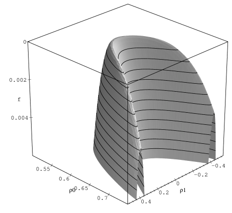
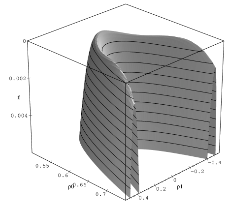
FIG. 14.: Moment free energy $f_{\rm m}(\rho_{0},\rho_{1})$ near the tricritical point, for the same parent as in Fig. 13. For ease of visualization, the free energy surface is shown upside down, with $f_{\rm m}$ increasing in the downward direction. (a) At the tricritical point $\chi^{\prime}=2.5$, the parent is stable (note that linear terms have been added to the free energy to make the tangent plane at the parent horizontal). (b) As $\chi^{\prime}$ is increased into the three-phase region (here $\chi^{\prime}=2.65$), the parent splits continuously into three phases.

We conclude this section with another illustration of the geometrical intuition which the moment free energy can provide. In Fig. 14, we plot the moment free energy $f_{\rm m}(\rho_{0},\rho_{1})$, eq. (103), for the uniform parent $\rho^{(0)}(\sigma)$ studied above. Two values of $\chi^{\prime}$ are shown: the tricritical value ($\chi^{\prime}=2.5$), and a value just in the three-phase region ($\chi^{\prime}=2.65$); the developing three minima of the free energy can clearly be seen. Even though the underlying polydisperse system has an infinite number of degrees of freedom $\rho(\sigma)$, the moment method thus gives us a tool for understanding and visualizing the occurrence of the tricritical point in terms of a simple free energy surface with two independent variables.

VI Conclusion

Polydisperse systems contain particles with an attribute $\sigma$ which takes values in a continuous range (such as particle size in colloids or chain length in polymers). They therefore have an infinite number of conserved densities, corresponding to a density distribution $\rho(\sigma)$. The fact that the free energy can depend on all details of $\rho(\sigma)$ makes the analysis of the phase behavior of such systems highly non-trivial. However, in many (especially mean-field) models the excess free energy only depends on a finite number of moment densities, i.e., (generalized) moments of $\rho(\sigma)$; the only dependence on other details of $\rho(\sigma)$ is through the ideal part of the free energy. For such models, which we call truncatable, we showed how a moment free energy can be constructed, which only depends on the moment densities appearing in the excess free energy. Two possible approaches for the construction of the moment free energy were described in Sec. II. The first, which we call the projection method (Sec. II A), is primarily geometrical; the second is mainly combinatorial (Sec. II B) and starts from first principles to derive an expression for the ideal part of the free energy in terms of moment densities. In Sec. II C, we showed that these two approaches give essentially equivalent results.

In Sec. III, we explored the properties of the moment free energy in detail. The moment free energy depends only on a finite number of moment densities, and can be used to predict phase behavior using the conventional methods known from the thermodynamics of finite mixtures. We showed that, for any truncatable model, this procedure yields the same spinodals, critical and multi-critical points as the original free energy, even though the latter depends on all details of the density distribution $\rho(\sigma)$. It also correctly predicts the onset of phase coexistence, i.e., the cloud points and corresponding shadows. Beyond the onset of phase coexistence (i.e., when one or more coexisting phases occupy comparable volumes), the results from the moment free energy are approximate, but can be made arbitrarily accurate by retaining additional moment densities in the moment free energy. We also explained how to check the local and global stability of a phase coexistence calculated from the moment free energy, and how the moment free energy reflects overall phase behavior in the space of density distributions $\rho(\sigma)$.

We discussed aspects of the numerical implementation of the moment free energy method in Sec. IV, highlighting its many advantages in terms of robustness, efficiency and stability. The method allows violations of the lever rule, but then ensures that these be kept small by adding $n-K$ extra moments (where $K$ is the number of moment densities actually present in the excess free energy of the underlying truncatable model). The solution of the phase equilibrium conditions thus proceeds in an $n$-dimensional space; but global (tangent plane) stability can always be verified by minimimization (of the tangent plane distance) in a space of dimension $K$. For $K>1$ exact minimization is not practicable, but standard search methods can instead be employed; we chose a Monte-Carlo type algorithm for this.

We then surveyed several sample applications in Sec. V. For length-polydisperse homopolymers (treated within Flory-Huggins theory), we showed explicitly how the moment free energy with only a single moment density (the volume fraction of polymer) gives the correct spinodals and critical points. By retaining the chain number density as an additional moment density, we could rationalize the behavior of cloud point and shadow curves as cuts through conventional two-species phase diagrams. As a second example, the case of copolymers with chemical polydispersity was considered, both without and with solvent. This gave us the opportunity to test the performance of the moment free energy method for multi-phase coexistence, and in particular to study how the accuracy of the predictions in the coexistence region increases as more and more moment densities are retained. In the presence of solvent, the same theory predicts a tricritical point under appropriate conditions, which was detected without problems, along with the associated three phase region, by our numerical algorithm. A plot of the two-moment free energy gave a simple geometrical picture of the origin of this tricritical point.

The results for the copolymer model showed that the log-error (97) can be used to decide when enough moment densities have been included to locate the correct number of phases and their compositions. For general purposes we suggest a log-error tolerance of order $10^{-4}$; this corresponds to limiting the rms lever-rule violations at the predicted phase coexistence (found by global minimization of the moment free energy) to 1% or so of the parent distribution. Given that in practice the parent is itself not known to such high precision, these violations lie well within an acceptable range of error. Indeed, every state of coexistence actually predicted by our algorithm represents the exact phase equilibrium of some or other parent, indistinguishable from the real one to within experimental accuracy. Here, as elsewhere in this paper, “exact” means exactly as predicted by a truncatable model free energy; such models are, of course, themselves approximate, which is another reason not to expend resources reducing the log-error below the level suggested above.

In summary, with exact results for cloud point and shadow curves, critical points and spinodals, as well as refinably accurate coexistence curves and multi-phase regions, the moment free energy method allows rapid and accurate computation of the phase behavior of many polydisperse systems. Moreover, by establishing the link to a projected free energy $f_{\rm m}(\rho_{i})$ which is a function of a finite set of conserved moment densities $\rho_{i}$, it restores to the problem much of the geometrical interpretation and insight (as well as the computational methodology) associated with the phase behavior of finite mixtures. This contrasts with many procedures previously in use for truncatable polydisperse systems [2, 3, 4, 5, 9, 10]. Some previous approximations to the problem have used (generalized) moments as thermodynamic coordinates; see e.g. [11, 14, 15, 17]. The moment free energy method provides a rational basis for these methods and, so long as the generalized moments are correctly chosen, guarantees that many properties of interest are found exactly. Note also that the commonplace method of “binning” the $\sigma$-distribution into discrete “pseudo-components” can be seen as a special case of the moment method in which each weight function is zero outside the corresponding bin; but since these moments do not, in general, coincide with those contained in the excess free energy the advantages described above are then lost.

We finish with some remarks about extensions to the moment method, within and outside the sphere of phase diagram prediction. First, methods of this type may extend to nontruncatable models, for which the excess free energy cannot be written directly in terms of a finite number of moments as in (6). For example, many mean-field theories correspond to a variational minimization of the free energy: $F\leq\langle E\rangle_{0}-TS_{0}$, where the subscript $0$ refers to a trial Hamiltonian [59]. In such a case, one might choose to first make a physically motivated decision about which (and how many) moment densities $\rho_{i}$ to keep, and then include among the variational parameters the “transverse” degrees of freedom of the density distribution $\rho(\sigma)$. We have not pursued this approach, though it may form a promising basis for future developments. Secondly, we note that physical insight based on moment free energies may increasingly play a part in understanding kinetic problems. For example, one of us [60] has argued that in many systems the zeroth moment (mean particle density) can relax more rapidly (by collective diffusion) than can the higher moments (by interdiffusion of different species), and that this may lead to novel kinetics in certain areas of the phase diagram. And finally, we point to recent work [61] in which the moment method has been extended, via density functional theory, to allow study of inhomogeneous states; this opens the way to studying the effect of polydispersity on interfacial tensions and other interfacial thermodynamic properties.

Acknowledgements: We thank P. Bladon, N. Clarke, R. M. L. Evans, T. McLeish, P. Olmsted, I. Pagonabarraga, W. C. K. Poon and R. Sear for helpful discussions. PS is grateful to the Royal Society for financial support. This work was also funded in part under EPSRC GR/M29696 and GR/L81185.

A Moment (Gibbs) free energy for fixed pressure

In this appendix, we explain how the construction of the moment free energy is extended to scenarios where the pressure (rather than the overall system volume) is held constant. One then describes the system by the particle number distribution $N(\sigma)=V\rho(\sigma)$; this is normalized so that its integral gives the total number of particles, $N=\int\!d\sigma\,N(\sigma)$. The relevant thermodynamic potential is the Gibbs free energy $G=\min_{V}F+\Pi V$, which we now construct. For a truncatable system, whose free energy density obeys eqs. (3,4) by definition, the Helmholtz free energy can be written as

$\displaystyle F=T\int\!d\sigma\,N(\sigma)\left[\ln\frac{N(\sigma)}{V}-1\right]+\tilde{F}$

where the excess free energy $\tilde{F}(N_{i},V)=V\tilde{f}(\rho_{i})$ depends on volume $V$ and on the moments $N_{i}=V\rho_{i}=\int\!d\sigma\,N(\sigma)w_{i}(\sigma)$ of the particle number distribution. If $\tilde{F}=0$, a Legendre transform gives the Gibbs free energy of an ideal mixture:

$\displaystyle G_{\rm id}=\min_{V}F_{\rm id}+\Pi V=T\int\!d\sigma\,N(\sigma)\ln\frac{\Pi N(\sigma)}{NT}=NT\int\!d\sigma\,n(\sigma)\ln n(\sigma)+NT\ln\frac{\Pi}{T}$

Here $n(\sigma)=N(\sigma)/N=\rho(\sigma)/\rho$ is the normalized particle distribution. In the general case, we split off the ideal part

$\displaystyle G=G_{\rm id}+\tilde{G}=\min_{V}F+\Pi V$

and obtain for the excess Gibbs free energy

$\displaystyle\tilde{G}=\min_{V}NT\ln\frac{NT}{\Pi V}+\tilde{F}(N_{i},V)+\Pi V$

This is a function of $N$ and the $N_{i}$ (as well as the fixed control parameters $\Pi,T$, which we suppress in our notation). We can therefore write the excess Gibbs free energy per particle, $\tilde{G}(N_{i},N)/N=\tilde{g}(m_{i})$, as a function of the moments $m_{i}=N_{i}/N$ ($i=1\ldots K$) of the normalized particle distribution $n(\sigma)$. Altogether, the Gibbs free energy per particle of a truncatable system becomes

$$g[n(\sigma)]=G/N=T\int\!d\sigma\,n(\sigma)\ln n(\sigma)+T\ln\frac{\Pi}{T}+\tilde{g}(m_{i})$$ (A1)

This has again a truncatable structure; the excess part $\tilde{g}$ “inherits” its moment structure from $\tilde{f}$. Note that because of the normalization of the $m_{i}$, $\tilde{g}$ does not depend on the density $\rho\equiv\rho_{0}$. It is therefore normally a function of one less variable than $\tilde{f}$, unless $\tilde{f}$ is already independent of $\rho$ (as is the case in Flory-Huggins theory, eq. (71), for example). The chemical potentials $\mu(\sigma)$ follow from (A1) as

$$\mu(\sigma) = \frac{\delta}{\delta N(\sigma)}Ng[N(\sigma)/N]$$ (A2)

$$= \frac{\delta g}{\delta n(\sigma)}+g-\int\!d\sigma^{\prime}\,n(\sigma^{\prime})\frac{\delta g}{\delta n(\sigma^{\prime})}$$ (A3)

$$= T\ln n(\sigma)+\sum_{i}w_{i}(\sigma)\frac{\partial\tilde{g}}{\partial m_{i}}+\left[T\ln\frac{\Pi}{T}+\tilde{g}-\sum_{i}m_{i}\frac{\partial\tilde{g}}{\partial m_{i}}\right]$$ (A4)

Multiplying by $n(\sigma)$ and integrating over $\sigma$, one has $g=\int\!d\sigma\,\mu(\sigma)n(\sigma)$ as it should be (compare eq. (A1)). Comparing (A4) with (48), one deduces that

$\displaystyle\frac{\partial\tilde{g}}{\partial m_{i}}=\tilde{\mu}_{i}$

and that the density $\rho$ of a phase with moments $m_{i}$ is given by

$\displaystyle T\ln\left(\frac{T\rho}{\Pi}\right)=\tilde{g}-\sum_{i}m_{i}\tilde{\mu}_{i}.$

To construct the moment Gibbs free energy, one can now proceed as in the constant volume case: in the ideal contribution, we replace $\ln n(\sigma)\to\ln[n(\sigma)/n^{(0)}(\sigma)]$, with a normalized parent distribution $n^{(0)}(\sigma)$, and then minimize $g$ at fixed values of the $m_{i}$. The minimum occurs for distributions $n(\sigma)$ from the family

$$n(\sigma)=n^{(0)}(\sigma)\exp\left(\lambda_{0}+\sum_{i}\lambda_{i}w_{i}(\sigma)\right)$$ (A5)

The extra Lagrange multiplier $\lambda_{0}$ comes from the normalization condition $m_{0}=\int\!d\sigma\,n(\sigma)=1$. Inserting into (A1), one obtains the moment Gibbs free energy

$$g_{\rm m}(m_{i})=T\left(\lambda_{0}+\sum_{i}\lambda_{i}m_{i}\right)+T\ln\frac{\Pi}{T}+\tilde{g}(m_{i})$$ (A6)

where the $m_{i}$ are given by

$\displaystyle m_{i}=\int\!d\sigma\,w_{i}(\sigma)n^{(0)}(\sigma)\exp\left(\lambda_{0}+\sum_{i}\lambda_{i}w_{i}(\sigma)\right)=\frac{\int\!d\sigma\,w_{i}(\sigma)n^{(0)}(\sigma)\exp\left(\sum_{i}\lambda_{i}w_{i}(\sigma)\right)}{\int\!d\sigma\,n^{(0)}(\sigma)\exp\left(\sum_{i}\lambda_{i}w_{i}(\sigma)\right)}$

The derivatives of $g_{\rm m}$ can again be identified as moment chemical potentials and obey

$$\mu_{i}\equiv\frac{\partial g_{\rm m}}{\partial m_{i}}=T\lambda_{i}+\frac{\partial\tilde{g}}{\partial m_{i}}=T\lambda_{i}+\tilde{\mu}_{i}.$$ (A7)

The constraint $m_{0}=1$ does not affect this result because the partial derivative is taken with the values of all moments other than $m_{i}$ fixed anyway. For the same reason, the second derivatives of the ideal part of $g_{\rm m}$ are (up to a factor $T$) given by the inverse of the matrix of second-order normalized moments $m_{ij}$, by analogy with (46). (Note that the first row and column of the second-order moment matrix, corresponding to $i=0$ or $j=0$, need to be retained; they can only be discarded after the inverse has been taken.)

From (A4), one deduces immediately that if one of a number of coexisting phases is in the family (A5), then so are all others. Equality of the exact chemical potentials $\mu(\sigma)$ in all phases is then equivalent to equality of the quantities

$$\tilde{\mu}_{i}+T\lambda_{i}=\mu_{i}\quad(i=1\ldots K),\qquad T\lambda_{0}+\tilde{g}-\sum_{i}m_{i}\tilde{\mu}_{i}.$$ (A8)

But from (A6,A7), these are simply the moment chemical potentials $\mu_{i}=\partial g_{\rm m}/\partial m_{i}$ and (up to an unimportant additive constant) the associated Legendre transform $g_{\rm m}-\sum_{i}m_{i}\mu_{i}$. Therefore, phase equilibria can be constructed by applying the usual tangent plane construction to the moment Gibbs free energy, in analogy with the constant volume case. Note, however, that this tangent plane construction now takes place in the space of the normalized moments $m_{i}$, rather than that of the unnormalized moment densities $\rho_{i}$. As pointed out above, this generically reduces the dimension by one. For the trivial case of a monodisperse system, $\tilde{f}$ is a function of $\rho$ only and $\tilde{g}$ does not depend on any density variables at all, so that the tangent plane condition becomes void as expected.

The exactness statements in Sec. III can also be directly translated to the constant pressure case. The arguments above imply directly that the onset of phase coexistence is found exactly from the moment Gibbs free energy: all phases are in the family (A5), because one of them (the parent) is, and the requirement of equal chemical potentials is satisfied. Spinodals and (multi-) critical points are also found exactly. Arguing as in Sec. III A, and using the vector notation of (56), the criterion for such points is found as

$$\Delta\mbox{\boldmath$\mu$}\equiv\mbox{\boldmath$\mu$}(\mbox{\boldmath$n$}(\epsilon))-\mbox{\boldmath$\mu$}(\mbox{\boldmath$n$}^{(0)})={\mathcal{O}}(\epsilon^{l})$$ (A9)

where $l=2$ for a spinodal and $l=2n-1$ for an $n$-critical point. Again, the curve $\mbox{\boldmath$n$}(\epsilon)$ only has to pass through phases with equal chemical potentials and can therefore be chosen to lie within the family (A5). As discussed above (eq. (A8)), the chemical potential difference on the left hand side of (A9) is then zero to the required order in $\epsilon$ if the same holds for the $\Delta\mu_{i}$ and $\Delta h$, where $h=g_{\rm m}-\sum_{i}m_{i}\mu_{i}$. It may look as if the constraint on $h$ gives one more condition here than in the constant volume case; but in fact $\Delta\mu_{i}={\mathcal{O}}(\epsilon^{l})$ for all $i$ already implies that $\Delta g_{\rm m}={\mathcal{O}}(\epsilon^{l+1})$ and hence $\Delta h={\mathcal{O}}(\epsilon^{l})$. The exact condition (A9) for spinodals and critical points is therefore again equivalent to the same condition obtained from the moment Gibbs free energy.

B Moment entropy of mixing and large deviation theory

In this appendix, we discuss some interesting properties of the Legendre transform result (31) for the moment entropy of mixing, in particular its relation to large deviation theory (LDT).

We first note that (31), which we derived by taking the limit $x\to 0$ of the result (28) for general $x$, can also be obtained by a more direct route. In the limit $x\to 0$, the sizes of particles in the smaller system become independent random variables drawn from $n^{(0)}(\sigma)$; the second phase can be viewed as a reservoir to which the small phase is connected. One writes the moment generating function for ${\cal P}(m)$ in the small phase as a product of $xN$ independent moment generating functions of $n^{(0)}(\sigma)$, and evaluates the integral over ${\cal P}(m)$ by a saddle point method [36].

One can also view (31) as a generalisation of Cramér’s large deviation theory (LDT) [62]. Recall that this theory treats the “wings” of a distribution like ${\cal P}(m)$ correctly, to which the central limit theorem (CLT) does not apply [63]. However, the CLT approximation in this problem has quite a beautiful interpretation, and is worth describing separately. It can be derived by assuming that $n^{(0)}(\sigma)$ is itself a Gaussian in eq. (31), or just written down directly:

$\displaystyle{\cal P}(m)\sim\exp\left[-N\frac{(m-m^{(0)})^{2}}{2\,v^{(0)}}\right]$

where $v^{(0)}$ is the variance of the parent distribution. We see that this gives a term in the free energy of the form

$\displaystyle\Delta f=-T\rho s=\rho T\frac{(m-m^{(0)})^{2}}{2\,v^{(0)}}.$

This result states that there is an entropic spring term in the free energy that penalizes deviations of the mean size $m$ from the mean size in the parent distribution. The spring constant is inversely proportional to the variance in the parent distribution, thus if the parent is narrower, it is harder to move away from the parental mean size [64]. However, as indicated above, the CLT is not sufficiently accurate for our purposes. For instance it gives a finite weight to $m<0$ even if $w(\sigma)$ is strictly positive. That said, the CLT may be attractive for narrow size distributions, and one might make a connection with the recent results of Evans et al [65] (even though the latter do not seem to rely on a specific shape of the distribution). We have not fully explored this avenue.

C Spinodal criterion from exact free energy

In this appendix, we apply the spinodal criterion (53) to the exact free energy (41) and show that it can be expressed in a form identical to (58). This result has been given by a number of authors [11, 12, 44], but we include it here for the sake of completeness.

Choosing for $\rho$ the vector $\rho(\sigma)$ (whose “components” are the values of $\rho(\sigma)$ for all $\sigma$), the spinodal criterion (53) applied to (41) becomes

$$\int\!d\sigma^{\prime}\,\frac{\delta^{2}f}{\delta\rho(\sigma)\delta\rho(\sigma^{\prime})}\,\delta\rho(\sigma^{\prime})=\sum_{i,j}\frac{\partial^{2}\tilde{f}}{\partial\rho_{i}\partial\rho_{j}}\,w_{i}(\sigma)\,\delta\rho_{j}+T\,\frac{\delta\rho(\sigma)}{\rho(\sigma)}=0$$ (C1)

The change of $\ln\rho(\sigma)$ along the instability direction (which is $\delta\rho(\sigma)/\rho(\sigma)$) is therefore a linear combination of the weight functions $w_{i}(\sigma)$. This means that the instability direction is within the family (42), consistent with our general discussion in Sec. III A. One can now rewrite (C1) in the form

$$\delta\rho(\sigma)=-\beta\sum_{i,j}w_{i}(\sigma)\,\rho(\sigma)\,\frac{\partial^{2}\tilde{f}}{\partial\rho_{i}\partial\rho_{j}}\,\delta\rho_{j}$$ (C2)

and take the moment with the $k$-th weight function $w_{k}(\sigma)$ to get

$\displaystyle\delta\rho_{k}+\beta\sum_{i,j}\rho_{ki}\frac{\partial^{2}\tilde{f}}{\partial\rho_{i}\partial\rho_{j}}\,\delta\rho_{j}=0.$

As promised, this is identical to the spinodal condition (58) derived from the moment free energy, with the matrix multiplications written out explicitly.

D Determinant form of critical point criterion

In this appendix, we give the form of the critical point criterion (60) that uses the spinodal determinant $Y$ from (58) [34]. At a critical point, the instability direction connects two neighboring points on the spinodal. The first order variation of the spinodal determinant $Y$ along this direction must therefore vanish. This gives

$$\delta Y=\sum_{i}\frac{\partial Y}{\partial\rho_{i}}\,\delta\rho_{i}+\sum_{i\leq j}\frac{\partial Y}{\partial\rho_{ij}}\,\delta\rho_{ij}=0.$$ (D1)

Here the $\delta\rho_{ij}$ are the changes in the second order moment densities along the instability direction. We can express these as a function of the $\delta\rho_{i}$ via the change in the Lagrange multipliers $\lambda_{i}$: From the definition (43), a change in the $\lambda_{i}$ changes the first and second order moment densities according to

$$\frac{\partial\rho_{i}}{\partial\lambda_{j}}=\rho_{ij}=\mbox{\boldmath$M$}_{ij},\quad\frac{\partial\rho_{ij}}{\partial\lambda_{k}}=\rho_{ijk}.$$ (D2)

Hence changes in second and first order moment densities are related by

$\displaystyle\delta\rho_{kl}=\sum_{i}\rho_{kli}\,\delta\lambda_{i}=\sum_{ij}\rho_{kli}\,(\mbox{\boldmath$M$}^{-1})_{ij}\,\delta\rho_{j}$

Inserting this into (D1) gives the determinant form of the critical point condition

$$\sum_{i}\frac{\partial Y}{\partial\rho_{i}}\,\delta\rho_{i}+\sum_{ij}\sum_{k\leq l}\frac{\partial Y}{\partial\rho_{kl}}\,\rho_{kli}\,(\mbox{\boldmath$M$}^{-1})_{ij}\,\delta\rho_{j}=0.$$ (D3)

Of course, if in an application of the moment free energy method one succeeds in calculating $Y$ explicitly as a function of the $\rho_{i}$ alone (rather than as a function of the $\rho_{i}$ and the $\rho_{ij}$), then one can determine critical points simply from the condition

$\displaystyle\delta Y=\sum_{i}\frac{dY}{d\rho_{i}}\,\delta\rho_{i}=0.$

We have written a total derivative sign here to indicate that the dependence of $Y$ on the $\rho_{ij}$ is accounted for implicitly.

REFERENCES

- [1] R. T. DeHoff, Thermodynamics in Material Science (McGraw-Hill, New York, 1992).
- [2] B. J. Bauer, Polymer Eng. Sci. 25, 1081 (1985).
- [3] M. T. Rätzsch and C. Wohlfarth, Adv. Polymer Sci. 98, 49 (1991).
- [4] A. Nesarikar, M. Olvera de la Cruz, and B. Crist, J. Chem. Phys. 98, 7385 (1993).
- [5] K. Solc, Makromol. Chem.-Macromol. Symp. 70-1, 93 (1993).
- [6] Some components of can also be discrete. For example, in a blend of two homopolymers A and B, both of which are length-polydisperse, one would choose , where is the chain length and labels polymer A and B, respectively. All integrations are then to be read as the combined sum and integral .
- [7] P. A. Irvine and J. W. Kennedy, Macromol. 15, 473 (1982).
- [8] J. J. Salacuse and G. Stell, J. Chem. Phys. 77, 3714 (1982).
- [9] K. Solc and R. Koningsveld, Coll. Czech. Chem. Comm. 60, 1689 (1995).
- [10] J. A. Gualtieri, J. M. Kincaid, and G. Morrison, J. Chem. Phys. 77, 521 (1982).
- [11] P. Irvine and M. Gordon, Proc. R. Soc. London A 375, 397 (1981).
- [12] S. Beerbaum, J. Bergmann, H. Kehlen, and M. T. Rätzsch, Proc. R. Soc. London A 406, 63 (1986).
- [13] E. M. Hendriks, Ind. Eng. Chem. Res. 27, 1728 (1988), Results in this paper formalize and summarize many earlier studies (and were rediscovered in several later ones).
- [14] E. M. Hendriks and A. R. D. Vanbergen, Fluid Phase Eq. 74, 17 (1992).
- [15] R. L. Cotterman and J. M. Prausnitz, Ind. Eng. Chem. Proc. Des. Dev. 24, 434 (1985).
- [16] S. K. Shibata, S. I. Sandler, and R. A. Behrens, Chem. Eng. Sci. 42, 1977 (1987).
- [17] P. Bartlett, J. Chem. Phys. 107, 188 (1997).
- [18] J. M. Kincaid, K. B. Shon, and G. Fescos, J. Stat. Phys. 57, 937 (1989).
- [19] M. L. Michelsen, Fluid Phase Eq. 33, 13 (1987).
- [20] M. L. Michelsen, Fluid Phase Eq. 9, 1 (1982).
- [21] R. L. Cotterman, R. Bender, and J. M. Prausnitz, Ind. Eng. Chem. Proc. Des. Dev. 24, 194 (1985).
- [22] M. L. Michelsen, Ind. Eng. Chem. Proc. Des. Dev. 25, 184 (1986).
- [23] M. L. Michelsen, Fluid Phase Eq. 30, 15 (1986).
- [24] M. L. Michelsen, Computers & Chemical Engineering 18, 545 (1994).
- [25] M. L. Michelsen, Fluid Phase Eq. 98, 1 (1994).
- [26] N. Clarke, T. C. B. McLeish, and S. D. Jenkins, Macromol. 28, 4650 (1995).
- [27] The parts of the CPC where the incipient phase has higher or lower density than the original phase are sometimes referred to as dew and bubble curve, respectively.
- [28] In systems containing solvent whose degrees of freedom have been eliminated (integrated out) from the free energy, this pressure is the osmotic pressure.
- [29] T. Boublik, J. Chem. Phys. 53, 471 (1970).
- [30] G. A. Mansoori, N. F. Carnahan, K. E. Starling, and T. W. Leland, Jr., J. Chem. Phys. 54, 1523 (1971).
- [31] P. Sollich and M. E. Cates, Phys. Rev. Lett. 80, 1365 (1998).
- [32] P. B. Warren, Phys. Rev. Lett. 80, 1369 (1998).
- [33] Formally, one can partition the space of all density distributions into equivalence classes, defined by having the same values for the moment densities . The moment subspace is then the space of these equivalence classes; the transverse subspace corresponds to variations of within a given equivalence class.
- [34] J. W. Gibbs, The Collected Works of J. Willard Gibbs; The Scientific Papers of J. Willard Gibbs, reprinted (Dover, New York, 1960).
- [35] In the standard notation of probability theory, the quantity should really be written as – the distribution of , given the fixed value of . Eq. (19) is then recognized as Bayes’ theorem.
- [36] An alternative development may be to express the desired quantities in terms of contour integrals in the complex plane, using Cauchy’s theory of residues, as described in E. Schrödinger, Statistical Thermodynamics, reprinted (Dover, New York, 1989). We have not explored this, mainly formal, development.
- [37] J. J. Salacuse, J. Chem. Phys. 81, 2468 (1984).
- [38] As expected, this is of the form required for an exact solution of the phase coexistence problem; compare (62).
- [39] The derivation of the moment entropy using the combinatorial method already suggests this property. The only difference is that we now treat the moment densities as conjugate to the Lagrange multipliers , whereas in the combinatorial derivation – which works with the normalized particle distribution – this role is played by the normalized moments . Compare eq. (31).
- [40] Note that if an analytic expression for in terms of the can be obtained, then derivatives such as can of course be evaluated directly in terms of the . The second order moments then never appear explicitly in the calculation.
- [41] M. E. Fisher and S. Zinn, J. Phys. A 31, L629 (1998).
- [42] To simplify matters, we make the common assumption that there is only a single instability direction. This implies that the coexisting phases have to meet along a line (curve). For the more general case, where two or more instability directions appear simultaneously, see [43].
- [43] G. R. Brannock, J. Chem. Phys. 95, 612 (1991).
- [44] J. A. Cuesta, Europhys. Lett. 46, 197 (1999).
- [45] P. B. Warren, Europhys. Lett. 46, 295 (1999).
- [46] S. Beerbaum, J. Bergmann, H. Kehlen, and M. T. Rätzsch, Proc. R. Soc. London A 414, 103 (1987).
- [47] Of course, this effective ‘prior’ is not known in advance (so the name is a slight misnomer); it can only be determined by an exact solution of the phase coexistence problem. As a consequence, it also changes as control parameters such as temperature are varied.
- [48] If we had a solution of the exact phase coexistence problem, this means that we can investigate its stability by checking only the TPD of a -dimensional family of density distributions (where is the number of moment densities in the excess free energy). It might then seem that the TPD does in fact play the role of a ‘low-dimensional’ (depending only on variables) free energy surface, in apparent contradiction to our statement that the exact phase coexistence solution does not permit such a low-dimensional interpretation. This paradox is resolved by noting that the TPD only ‘comes into existence’ once the full phase coexistence problem has been solved; unlike the moment free energy, it is not a given free energy surface from which the phase coexistence is derived by a tangent plane construction.
- [49] More explicitly, the exact free energy and TPD are convex w.r.t. the transverse degrees of freedom of ; local stability therefore only needs to be checked for the moment degrees of freedom, where again the moment free energy is sufficient.
- [50] W. H. Press, S. A. Teukolsky, W. T. Vetterling, and B. P. Flannery, Numerical Recipes in C (2nd ed.) (Cambridge University Press, Cambridge, 1992).
- [51] B. Hesselbo and R. B. Stinchcombe, Phys. Rev. Lett. 74, 2151 (1995).
- [52] P. J. Flory, Principles of Polymer Chemistry (Cornell, Ithaca, 1953).
- [53] This result can also be obtained by considering a system with solvent at fixed osmotic pressure (see App. A), and then taking the limit . Note that the normalized moment and the (unnormalized) moment density are identical for this model (and in our chosen units), because the dense limit corresponds to .
- [54] One might also have chosen the cross-entropy as an error measure; this corresponds to leaving out the square in (97), thus allowing cancellations between positive and negative values of the logarithm. In our numerical experiments, this tended to give misleadingly small values of .
- [55] One may expect intuitively that, starting from at the cloud point, should increase as one moves deeper into the coexistence region by increasing . We find that this is so, but only as an overall trend: when new phases are detected as is increased, may temporarily decrease before increasing again. This explains the crossing of the curves for and in Fig. 11.
- [56] One exception might be the case where the polydispersity variable can assume values from an infinite range (as in the length polydisperse polymer problem treated in Sec. V A, where there is no upper limit on ). The form of the formally exact solution (62) can then give information about the asymptotic behavior of the extra weight functions. We leave this issue for future work.
- [57] L. Leibler, Makromol. Chem.-Rapid Comm. 2, 393 (1981).
- [58] Note that our algorithm does not make use of the symmetry which could in principle be used to reduce the complexity of the three-phase coexistence problem to that of ordinary two-phase coexistence. The scenario therefore provides a genuine test of the multi-phase capabilities of the algorithm.
- [59] R. P. Feynman, Statistical Mechanics (Benjamin, Reading, MA, 1972).
- [60] P. B. Warren, Phys. Chem. Chem. Phys 1, 2197 (1999).
- [61] I. Pagonabarraga, M. E. Cates, and G. J. Ackland, , preprint cond-mat/9909339.
- [62] H. Cramér, Act. Sci. Indust. 736, 5 (1938); see also R. S. Ellis, Entropy, Large Deviations and Statistical Mechanics, (Springer, New York, 1985); for an accessible summary see U. Frisch and D. Sornette, J. Physique 7 (1997) 1755.
- [63] The CLT only claims that converges to a Gaussian if one simultaneously rescales by , and is thus strictly limited to the region . LDT, on the other hand, addresses the asymptotic behaviour of the Cramér ‘rate function’ for all .
- [64] In polymer theory, the LDT result corresponds to the theory of large chain extensions: P. J. Flory, Statistical Mechanics of Chain Molecules, (Interscience, New York, 1969). Another mapping exists onto Debye’s theory for dielectric properties of molecules with permanent dipoles: P. Debye, Polar Molecules, reprinted (Dover, New York, 1958).
- [65] R. M. L. Evans, D. J. Fairhurst, W. C. K. Poon, Phys. Rev. Lett. 81 (1998) 1326.