A modified dual-slope method for heat capacity measurements of condensable gases

Abstract

A high resolution non-adiabatic method for measuring the heat capacity ($C_{v}$) of bulk samples of condensable gases in the range 7.5-70 K is described. In this method $C_{v}$ is evaluated by directly comparing the heating and cooling rates of the sample temperature for two algebraically independent heat pulse sequences without explicit use of the thermal conductance between sample and thermal bath. A fully automated calorimeter for rapid measurement of $C_{v}$ of molecular solids utilizing this technique is presented.

]

I INTRODUCTION

The adiabatic heat-pulse calorimetry has been widely used to investigate the thermodynamic properties of materials for more than a century. The applied principle, $C=\triangle Q/\triangle T$, which describes the heat capacity $C$ of the sample, is determined by the pulse heat $\triangle Q$ supplied to the sample under adiabatic conditions and the temperature rise $\triangle T$, is well known.[1, 2] Due to the inherent simplicity as well as the general applicability independent of the sample thermal conductivity, this method is the most favored choice for heat capacity measurements of condensable gases which have poor thermal conductivity in their low temperature solid phase.[3, 4, 5] Although the traditional adiabatic calorimetry has high precision and can be used to determine the latent heat at strong first-order transitions, it is very difficult to achieve the resolution needed to characterize the temperature dependence of $C_{v}(T)$ (or $C_{p}(T)$) close to the critical temperature $T_{c}$ for a second-order transition. Also, because of the inherent limitations on achieving the ideal adiabatic conditions at low temperatures and the long time required to cover a few tens of kelvin temperature range with reasonable number of data points, new user friendly non-adiabatic techniques [6, 7, 8, 9, 10, 11, 12, 13] with excellent sensitivity are needed to study the heat capacity of condensable gases. Among these new techniques, the most sensitive method is the ac method devised by Sullivan and Seidel.[6] While the ac method allows one to obtain accurate values of $C_{v}$, it suffers from the fact that it normally must be used for small samples at low ac frequencies and over limited temperature ranges (typically $T<20$ K). In order to keep the sample in equilibrium with the heater and thermometer during one cycle, the time constant for thermal relaxation ($\tau_{1}$) of the sample plus sample holder (or calorimeter) to the thermal reservoir must be short compared to the period of the driving flux. In addition, the samples’s internal equilibrium time constant ($\tau_{2}$) with the sample holder (or calorimeter) must be short compared to $\tau_{1}$. It is this latter constraint which restricts the applicability of this method to small samples with sufficiently large thermal conductivity such as pure metals below 20 K.

A slightly less sensitive method involving a fixed heat input followed by a temperature decay measurement is the relaxation method. [7, 14, 15] In this method the sample is raised to an equilibrium temperature above the thermal reservoir and then allowed to relax to the reservoir temperature without heat input. A recent improvement of this technique utilizing advanced numerical methods was provided by Hwang $et$ $al.$[12] The relaxation method requires extensive calibration of the heat losses of the sample as a function of temperature difference between the reservoir and the final sample temperature and relies on accurate, smooth temperature calibration of thermometers. The technique depends heavily on the numerical techniques used to determine many equilibrium heat losses during the heating portion of the relaxation cycle to obtain good temperature resolution of the heat capacity changes. Though Hwang $et$ $al.$[12] addressed the problems arising from large $\tau_{2}$, this method still fails to provide accurate $C_{v}$ values above $\sim$20 K for large samples with poor thermal conductivity.

A variation of the relaxation method called dual-slope method, was first discussed by Riegel and Weber.[8] In this method an extremely weak thermal link to the reservoir is used and the temperature of the sample is recorded over a 10 h. cycle while heating at constant power for one half of the cycle, and then allowing the sample relax with zero heat input. The heat loss to the reservoir and surroundings can be eliminated from the calculation of $C_{v}(T)$ using this technique provided the sample, sample holder, and the thermometer are always in equilibrium with each other (the reason for long 10 h. cycle to cover 3 K range), and the reservoir temperature is held constant over the 10 h. cycle. A further modification of this technique is a hybrid between the ac method and the dual-slope method,[9] which reduces the duration of the cycle to about two hours. Although the dual-slope method is very elegant and easy to implement, the technique has only been implemented for small samples (typically less than 0.5 g) with good thermal conductivity and at temperatures less than $\sim$20 K. The success of this method depends heavily on achieving very good thermal equilibrium between the sample, sample holder, and the thermometer, and for large samples with poor thermal conductivity (i.e., large $\tau_{2}$) this method may also fail when we consider only the first order approximation of the heat balance equations of Riegel and Weber.[8, 9, 12]

In the case of condensable gases, the sample size must be at least a few grams to reduce the spurious effect of sample condensed in the fill line and the heat leak through this tube. Due to the low thermal conductivity of these samples, in particular for powdered samples which may not wet the calorimeter walls, the $\tau_{2}$ can be very large leading to the failure of most of the above techniques. The present article describes a modified dual-slope method in which $C_{v}$ is evaluated by directly comparing the heating and cooling rates of the sample temperature for two algebraically independent heat pulse sequences without explicit use of the thermal conductance between sample and thermal bath. For the specific geometry of the calorimeter that we used, which is most suitable for the heat capacity measurements of condensable gases in the presence of external electric or magnetic fields, higher order heat balance equations are calculated, which can easily be adapted for other sample configurations as well. Because of the explicit consideration of the higher order equations, the problem of large $\tau_{2}$ is naturally addressed and during the heating and cooling cycles one does not require the sample to be in equilibrium with the thermometer, or in other words, the thermometer need not necessarily record the actual sample temperature. Due to this freedom we can obtain $C_{v}$ of samples with poor thermal conductivity very rapidly.

II Theory

To model the thermal response of a heat-pulse calorimeter (Fig. 2) for heat capacity measurements, with the schematic diagram shown in Fig. 1, where the calorimeter is heated with the application of heater power $P(t)$ to some desired temperature $T_{max}$ and then allowed to cool-down, we start with the following set of heat balance equations:

$$P(t)=C^{\prime}\dot{T_{h}^{\prime}}+\lambda_{s}(T_{h}^{\prime}-T_{h})+\lambda_{r}(T_{h}^{\prime}-T_{0})$$ (1)

and

$$0=C\dot{T_{h}}+\lambda_{s}(T_{h}-T_{h}^{\prime})-P_{0}(T_{h})$$ (2)

for heating, and

$$0=C^{\prime}\dot{T_{c}^{\prime}}+\lambda_{s}(T_{c}^{\prime}-T_{c})+\lambda_{r}(T_{c}^{\prime}-T_{0})$$ (3)

and

$$0=C\dot{T_{c}}+\lambda_{s}(T_{c}-T_{c}^{\prime})-P_{0}(T_{c})$$ (4)

for cooling, where $C$ and $T$ are the heat capacity and the temperature of the thermometer well plus the inner conductor respectively, $C^{\prime}$ and $T^{\prime}$ are those of the outer conductor plus the heater coil. From these equations we need to obtain the quantity $(C+C^{\prime})$ which is the net heat capacity of the calorimeter. Once the sample is condensed in the calorimeter, both $C$ and $C^{\prime}$ will be modified but the above equations are still valid. $P_{0}(T)$ is the parasitic stray heat due to the conduction of heat through the fill line, the stainless steel suspension rod, and the thermometer leads as well as radiation from the pumping line. From the geometry of the calorimeter (Fig. 2) it is reasonable to assume that this stray heat affects only the inner conductor heat balance equations (Eqs. 2 & 4).

Since the thermometer is firmly coupled to the inner conductor through the thermometer well, the temperature $T$ is what the thermometer practically records. Hence we need to eliminate $T^{\prime}$ to obtain $(C+C^{\prime})$. For $T_{h}=T_{c}$ Eqs. 1 & 3 reduce to

$$P(t)=C^{\prime}(\dot{T_{h}^{\prime}}-\dot{T_{c}^{\prime}})+(\lambda_{s}+\lambda_{r})(T_{h}^{\prime}-T_{c}^{\prime}).$$ (5)

From Eqs. 2 & 4 and their first derivatives we obtain

$$(T_{h}^{\prime}-T_{c}^{\prime})=\frac{C}{\lambda_{s}}(\dot{T_{h}}-\dot{T_{c}}),$$ (6)

$$(\dot{T_{h}^{\prime}}-\dot{T_{c}^{\prime}})=(\dot{T_{h}}-\dot{T_{c}})+\frac{C}{\lambda_{s}}(\ddot{T_{h}}-\ddot{T_{c}}).$$ (7)

After eliminating $T_{h}^{\prime}$, $T_{c}^{\prime}$ and their time derivatives from Eqs. 5, 6, and 7 we obtain

$$P(t)=(C+C^{\prime})(\dot{T_{h}}-\dot{T_{c}})+\frac{CC^{\prime}}{\lambda_{s}}(\ddot{T_{h}}-\ddot{T_{c}})+\frac{C\lambda_{r}}{\lambda_{s}}(\dot{T_{h}}-\dot{T_{c}}).$$ (8)

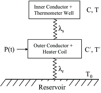
FIG. 1.: Simplified diagram of the thermal system of sample, sample holder, and thermal bath. The thermal link between the outer conductor plus heater of heat capacity $C^{\prime}$ at temperature $T^{\prime}$ and temperature-controlled reservoir bath at $T_{0}$ is represented by the thermal conductance $\lambda_{r}$. $\lambda_{r}$ may be controlled by changing the He exchange gas pressure. The heater input power $P(t)$ is obtained from a waveform generator and a suitable power amplifier. The thermal link (through the sample) between the inner conductor plus thermometer well of heat capacity $C$ at temperature $T$ and the outer conductor is represented by the thermal conductance $\lambda_{s}$.

Clearly, Eq. (8) reduces to the first order derivations of Riegel and Weber[8] for $\lambda_{s}\gg 1$. However, for condensed gases, in particular for powdered samples, this condition is never met. In the present geometry, for a sufficiently weak thermal link $\lambda_{r}$ where $\lambda_{s}\gg\lambda_{r}$, one can ignore the last term in Eq. (8). To solve the remaining equation exactly for $C+C^{\prime}$, we need to obtain Eq. (8) for two algebraically independent pulse sequences of $P(t)$.

III Experiment

Figure 2 shows the design of the calorimeter optimized for the above technique. The thermal reservoir is made up of a brass vacuum can (18 cm long, 4 cm diameter) with a manganin wire wound uniformly on the entire length of the outer surface. A dilute solution of GE-varnish is used to soak the cloth insulation of the manganin heater wire to provide good thermal contact with the vacuum can. A grooved copper tube (4 cm long) is soldered to the top flange, which can be used for heat sinking the heater and thermometer wires before connecting them to the calorimeter. A 122 cm long stainless steel tube (0.96 cm diameter) is soldered to the top flange to pump the vacuum space as well as support the vacuum can. copper radiation baffles are placed inside this tube at regular intervals to reduce the thermal radiation. In addition the top flange supports up to ten individual vacuum feed-throughs (not shown), which are thermally anchored to the flange through STYCAST 2850FT vacuum seal which has good thermal conductivity at low temperatures. The calorimeter consists of two concentric, thin walled, gold plated, OFHC copper cylinders 10.2 cm in length providing a 1 mm cylindrical shell space for condensing the samples. This shell space is vacuum sealed at both ends with homemade 1 mm thick STYCAST 2850FT O-rings.[16] The outer conductor (2.7 cm inner diameter and 0.2 mm wall thickness) with a brass heater wire uniformly wound on the entire length of its outer surface serves as a radial heating element. Uniform winding of the heater wire is very crucial in eliminating longitudinal heat flow thereby reducing the temperature gradient along the length of the calorimeter. For good thermal contact with the outer cylinder, a dilute solution of GE-varnish was applied to the heater wire. In the middle of the inner conductor (2.5 cm diameter, 0.4 mm wall thickness) a thin copper ring as well as a copper thermometer well are soldered (see Fig. 2). The larger wall thickness (0.4 mm instead of 0.2 mm) for the inner cylinder is necessary to withstand the pressures generated when the solid samples melt at high temperatures. The copper ring sandwiched between two threaded nylon wings supports the calorimeter when suspended from the top flange with the help of a threaded stainless steel rod. This arrangement not only reduces the unwanted heat leaks to the calorimeter but also provides excellent mechanical stability when the free end of the stainless steel rod is slipped into the post at the bottom of the vacuum can (see Fig. 2).

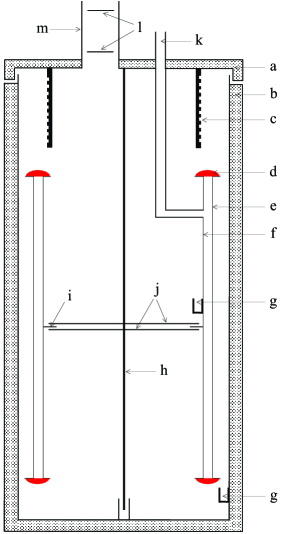
FIG. 2.: Cross section of the thermal reservoir and calorimeter. (a) Top flange with vacuum feed-throughs, (b) brass vacuum can with highly uniform heater wire wound on the outer surface, (c) 1.6 cm diameter copper tube with grooves on the outer surface, (d) STYCAST 2850FT seal,[16] (e) outer conductor with highly uniform heater wire wound on the outer surface, (f)inner conductor, (g) copper thermometer wells soldered to the walls, (h) threaded stainless steel rod, (i) 0.5 mm thick copper ring soldered to the inner conductor, (j) threaded nylon wings, (k) sample fill line, (l) copper radiation baffles, (m) stainless steel tube for support as well as pumping.

The 1.6 mm diameter cupronickel alloy tube serving as the sample fill line is coiled into a three turn spring (not shown) before soldering it to the inner cylinder. To be able to apply electric field across the sample cell when necessary, it is important to ground the outer conductor (to reduce electrical interference from the heater current) and apply the high voltage to the inner conductor. Hence the coiled section of the fill line is isolated electrically as well as thermally from the remaining length with the help of a vacuum joint made up of a wider cupronickel tube, cigarette paper, and STYCAST seal. To assist sample condensation, the manganin heater wire is wrapped on the fill line tube outside of the vacuum can. Two factory calibrated germanium resistance thermometers[17] placed inside the thermometer wells are used for recording the temperatures of the calorimeter and the thermal reservoir. The entire assembly is placed in a second vacuum can (125 cm long, 5 cm diameter) which can be lowered into a commercial liquid He dewar. With this arrangement including a few suitably placed copper radiation baffles at the neck of the outer vacuum can, a standard 100 liter dewar lasted for almost a month while heat capacity experiments were carried out in the $4.2-75$ K range.

IV RESULTS AND DISCUSSION

Our observations indicate that due to the high degree of cylindrical symmetry, even though the calorimeter is rather unusually long ($\sim$10 cm), thermometers record the expected temperature values to very high accuracy. Figure 3 shows typical temperature excursions when the calorimeter is filled with pure N₂ as a sample. For simplicity we chose square and triangular voltage pulses for two algebraically independent $P(t)$ sequences. Both pulses can be easily generated with the help of a standard signal generator or data acquisition card and a suitable operational amplifier. Before the heat pulse is applied, the calorimeter is left to equilibrate with the surroundings until its temperature trace is horizontal with the time axis. Typically, when the reservoir temperature is adjusted to a new value, the calorimeter attained equilibrium in 30 to 60 min. To ensure that the calorimeter always attained equilibrium from either a higher temperature or a lower temperature for all pulse sequences (i.e., $T\rightarrow T_{0}^{+}$ or $T\rightarrow T_{0}^{-}$), and that small hysteresis of the the thermometer does not affect the trace, when $T_{0}$ is set to a higher value, a small heat pulse is simultaneously applied to the calorimeter so that its temperature rises above the equilibrium temperature by at least 2 to 3 K. When such a precaution was not taken, we observed that the base line of the two traces in Fig. 3 differed by $\sim$100 mK resulting in spurious results when fit to Eq. (8).

Although we assumed that the last term in Eq. (8) will be negligible for $\lambda_{s}\gg\lambda_{r}$, it is clear that for the long exponential decay section of the traces (below the lower horizontal line in Fig. 3) where $(\dot{T_{h}}-\dot{T_{c}})$ can be very large, the above approximation may not be valid. We observed that for a typical 6.5 K pulse (similar to Fig. 3), the useful window of temperature where the above approximation is valid for obtaining faithful results is only 3.5$\sim$4 K (the section between the two dashed lines in Fig. 3). It is crucial that during the entire pulse sequence, the reservoir temperature $T_{0}$ should be constant. With the help of a program written in LabVIEW,[18] which controls the voltage across the reservoir heater through a multifunction AD/DA card[18] and with the thermometer output in the negative feedback loop, we were able to maintain $T_{0}$ to within 30 mK during the entire pulse sequence (see Fig. 3). Because the feedback is controlled through software, excellent stability in $T_{0}$ was achieved by changing the feedback parameters depending on the pulse height and temperature range.

Figure 4 shows the heat capacity curves of the calorimeter filled with pure N₂ for two $T_{0}$ values. Excellent overlap of the curves demonstrates that with this technique, we can obtain heat capacity of samples with poor thermal conductivity very rapidly ($\sim$3.5 K range in 3 h.), without further curve fitting generally required with other techniques.[9] By extending the LabVIEW program written for controlling the reservoir temperature $T_{0}$, we fully automated the data acquisition process to obtain pulse sequence data for various $T_{0}$ values with an interval of 2.5 K to ensure data overlap from adjacent pulse sequences. Once the data are obtained, standard third degree polynomial fits (only for the useful temperature interval similar to the one between dashed lines in Fig. 3) are employed for obtaining time derivatives in Eq. (8). Once the heat capacity is calculated for each pulse sequence, no further curve fitting is necessary and in general for $T<30$ K, the overlap between adjacent curves is better than the one shown in Fig. 4. Figure 5 shows the heat capacity of the empty calorimeter (with small amounts of He gas for better thermal contact) obtained through the above automated process in the $10-70$ K range. The kink at 60 K, the presence of which is accidental, shows the heat capacity near a continuous phase transition with excellent resolution. The data shown without further curve fitting clearly demonstrates the high sensitivity of the technique.

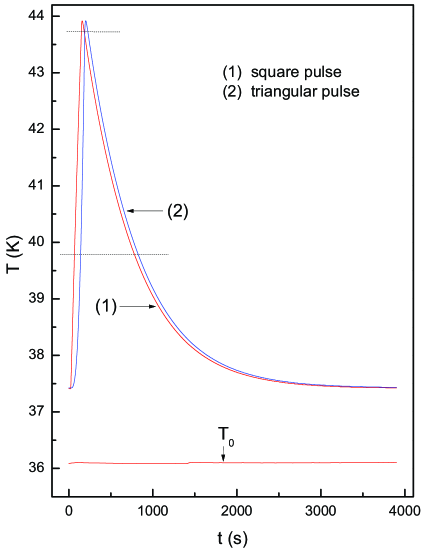
FIG. 3.: Traces of $T(t)$ and $T_{0}(t)$ for two heat pulses when the calorimeter is filled with pure N₂ sample. Useful interval for obtaining heat capacity is shown between two dashed lines. The difference between the trace of $T_{0}$ and the baseline of $T$ is due to $P_{0}$.

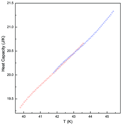
FIG. 4.: Heat capacity of the calorimeter filled with pure N₂ sample. Data are obtained for two pulse sequences with respective $T_{0}$ values separated by 2 K.

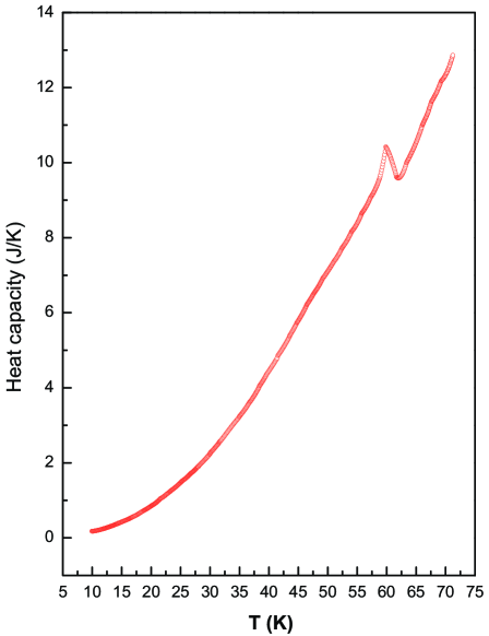
FIG. 5.: Heat capacity of the empty cell with small amounts of He exchange gas for better thermal contact. No curve fitting techniques are utilized as the adjacent heat pulse data overlap very well. The sharp kink at 60 K, whose origin is not known, clearly demonstrates the high resolution of the technique near continuous phase transitions.

In summary, we have demonstrated the use of a novel technique to study the heat capacity of moderately large samples with poor thermal conductivity in the 7.5-70 K range. A fully automated calorimeter for rapid measurement of the heat capacity of condensable gases utilizing the above technique has been presented. The technique along with the automated calorimeter with a provision to apply external electric and magnetic fields is particularly useful for the study of continuous phase transitions in molecular solids as well as field induced changes in the heat capacity.

- [1] A. Eucken, Z. Phys. 10, 586 (1909).
- [2] W. Nernst, Sitzb. Kgl. Preuss. Akad. Wiss. 12, 261 (1910).
- [3] M. T. Alkhafaji and A. D. Migone, Phys. Rev. B 53, 11 152 (1996).
- [4] M. I. Bagatskii, I. Y. Minchina, and V. G. Manzhelii, Sov. J. Low Temp. Phys. 10, 542 (1984).
- [5] L. G. Ward, A. M. Saleh, and D. G. Haase, Phys. Rev. B 27, 1832 (1983).
- [6] P. F. Sullivan and G. Seidel, Phys. Rev. 173, 679 (1968).
- [7] R. Bachmann, F. J. Disalvo, T. H. Geballe, R. L. Greeene, R. E. Howard, C. N. King, H. C. Kirsch, K. N. Lee, R. E. Schwall, H. U. Thomas, and R. B. Zubeck, Rev. Sci. Instrum. 43, 205 (1972).
- [8] S. Riegel and G. Weber, J. Phys. E: Sci. Instrum. 19, 790 (1986).
- [9] Jing-Chun Xu, C. H. Watson, and R. G. Goodrich, Rev. Sci. Instrum. 61, 814 (1990).
- [10] V. K. Pecharsky, J. O. Moorman, and K. A. Gschneidner, Rev. Sci. Instrum. 68, 4196 (1997).
- [11] H. Yao, K. Ema, and C. W. Garland, Rev. Sci. Instrum. 69, 172 (1998).
- [12] J. S. Hwang, K. J. Lin, and Cheng Tien, Rev. Sci. Instrum. 68, 94 (1997).
- [13] A. J. Jin, C. P. Mudd, N. L. Gershfeld, and K. Fukada, Rev. Sci. Instrum. 69, 2439 (1998).
- [14] E. M. Forgan and S. Nedjat, Rev. Sci. Instrum. 51, 411 (1980).
- [15] R. E. Schwall, R. E. Howard, and G. R. Stewart, Rev. Sci. Instrum. 46, 1054 (1975).
- [16] S. Pilla, J. A. Hamida, N. S. Sullivan, Rev. Sci. Instrum. 70, 4055 (1999).
- [17] Scientific Instruments Inc., 4400 W. Tiffany Drive, Mangonia Park, West Palm beach, FL 33407.
- [18] National Instruments Corporation, 11500 N. Mopac Expwy. Austin, TX 78759-3504.