Statistical mechanics approach to the phase unwrapping problem

Abstract

The use of Mean-Field theory to unwrap principal phase patterns has been recently proposed. In this paper we generalize the Mean-Field approach to process phase patterns with arbitrary degree of undersampling. The phase unwrapping problem is formulated as that of finding the ground state of a locally constrained, finite size, spin-L Ising model under a non-uniform magnetic field. The optimization problem is solved by the Mean-Field Annealing technique. Synthetic experiments show the effectiveness of the proposed algorithm.

PACS: 95.75.Kk , 95.75.-z , 45.10.Db

1 Introduction

The determination of the absolute phase from a fringe pattern is an important problem that finds applications in many areas: homomorphic signal processing [1], solid state physics [2], holographic interferometry [3], adaptive or compensated optics [4], magnetic resonance imaging [5] and synthetic aperture radar interferometry [6].

In all these applications one obtains a two-dimensional fringe pattern whose spatially-varying phase is related to the physical quantity to be measured. The computation of phase by any inverse trigonometric function (e.g. arctangent) provides only principal phase values, which lie between $\pm\pi$ radians. The process of phase unwrapping (PU), i.e. the addition of a proper integer multiple of $2\pi$ to all the pixels, must be carried out before the physical quantity can be reconstructed from the phase distributions. Since many possible absolute phase fields are compatible with a given fringe pattern, phase unwrapping is ill-posed in a mathematical sense: Hadamard [7] defined a mathematical problem to be well-posed if a unique solution exists that depends continuously on the data; in this case, the uniqueness requirement is violated.

Ill-posed problems arise frequently in many areas of science and engineering; well-known examples are analytic continuation, the Cauchy problem for differential equations, computer tomography, and many problems in image processing and machine vision that involve the reconstruction of images from noisy data.

The fact that a problem is not well-posed does not mean that it cannot be solved: rather, in order to be solved it must be first regularized by introducing additional constraints (prior knowledge) about the behaviour of the solution. Variational regularization corresponds to modeling the physical constraints of the problem by a suitable functional; the solution is then sought as the minimizer of this functional.

In the last years, an increasing interest has been devoted to adapt methods from Statistical Mechanics to nonconvex optimization problems arising from the variational regularization of ill-posed problems. Geman and Geman [8] suggested that the Ising model is applicable to image restoration through the Bayesian formalism. This problem corresponds to searching the ground state of a finite-size Ising model under a non-uniform external field. Geman and Geman applied this to the recovery of corrupted images by using simulated annealing of a spin-S Ising model. After that, Gidas [9] proposed a new method based on a combination of the renormalization group technique and the simulated annealing procedure; then, Zhang [10] introduced Mean-Field Annealing to treat the image reconstruction problem, while Tanaka and Morita [11, 12] applied the cluster variation method. Methods of statistical mechanics have also been used to study combinatorial optimization problems (see, e.g., [13] and references therein).

In a couple of recent papers, the phase unwrapping problem was handled by methods of Statistical Mechanics. Simulated annealing was applied in [14]. In [15] the problem is solved by the Mean-Field Annealing (MFA) technique; PU is formulated as a constrained optimization problem for the field of integer corrections to be added to the wrapped phase gradient in order to recover the true phase gradient, with the cost function consisting of second order differences, and measuring the smoothness of the reconstructed phase field. This is equivalent [15] to finding the ground state of a locally-constrained ferromagnetic spin-1 Ising model under a non-uniform external field. The optimization problem is then solved by MFA and consistent solutions are found in difficult situations resulting from noise and undersampling.

Mean Field Annealing is closely related to Simulated Annealing [8]. Both approaches formulate the optimization problem in terms of minimizing a cost function and defining a corresponding Gibbs distribution. Simulated Annealing then proceeds by sampling the Gibbs probability distribution as the temperature is reduced to zero, whereas MFA attempts to track an approximation of the mean of the same distribution.

The algorithm described in [15] was constructed under the assumption that the possible values for the correction field were restricted to belong to the set $\{-1,0,1\}$. In this paper we generalize the MFA algorithm to the case of a set $\{-L,\ldots,L\}$, with $L$ an arbitrary integer. The corresponding statistical system is a locally-constrained spin-L Ising model.

The present generalization allows the processing of input phase patterns with arbitrary degree of undersampling; our experiments on synthetic phase fields show the effectiveness of the proposed algorithm.

The paper is organized as follows. In sect. 2 the phase unwrapping problem is introduced and its ill-posedness is highlighted. In sect. 3 the deterministic MFA algorithm is described in detail. Then, in sect. 4 some experimental results on simulated phase fields are presented. Some conclusions are then drawn in sect. 5.

2 Phase Unwrapping Problem

We briefly recall here the phase unwrapping terminology, and refer the reader to [16] for a complete discussion.

Given an absolute phase pattern $f(x,y)$ on a two-dimensional square grid, what is actually measured is the wrapped phase field $g(x,y)$ which can be expressed in terms of the $f$ field through a wrapping operator, Wr, defined so that $g(x,y)$ always lies in the interval $[-\pi,+\pi)$:

$$g(x,y)=\mathrm{Wr}[f(x,y)]=\arg\left\{\exp[\mathrm{i}f(x,y)]\right\}.$$ (1)

Phase unwrapping means recovering the absolute phase field $f$, which is usually related to the physical quantity to be measured, from the knowledge of the $g$ field. This can be done in practice by estimating the absolute phase gradient from the wrapped phase field and integrating it throughout the 2-D grid. This simple method is effective only in absence of phase aliasing, i.e. if the phase field is correctly sampled.

In fact, if the Nyquist condition:

$$\left|\mathbf{\nabla}f(x,y)\right|<\pi,$$ (2)

where $\nabla$ is the discrete gradient, is verified everywhere on the grid, the absolute phase gradient is obtained by wrapping the gradient of the wrapped phase field, according to the formula:

$$\mathbf{A}(x,y)=\mathrm{Wr}[\mathbf{\nabla}g(x,y)].$$ (3)

As mentioned, if condition (2) is satisfied, one has:

$$\mathbf{\nabla}f(x,y)=\mathbf{A}(x,y),$$ (4)

and the $f$-pattern is obtained by integrating $\mathbf{A}$ along any path connecting all sites on the grid.

The Nyquist condition is often violated because of undersampling of the signal from which the principal phase is extracted. This can result either from system noise, or from critical values of the slopes of the physical surface which is analyzed through interferometry. For example, in the case of SAR interferometry, the surface is the portion of Earth imaged from the sensor (usually air- or satellite-borne), while noise can arise from sensor thermal electronic motion, or from other sources of electronic signal disturbances.

If the Nyquist condition is not satisfied everywhere on the grid, then the wrapped gradient $\mathbf{A}$ of the wrapped phase field is not assured to equal the absolute phase gradient. In this case, a more general relation must be written, rather than (4), i.e.:

$$\mathbf{\nabla}f(x,y)=\mathbf{A}(x,y)+2\pi\mathbf{k}(x,y),$$ (5)

where $\mathbf{k}(x,y)$ is a vector field of integers. In this case, solving PU amounts to finding the correct field $\mathbf{k}$.

Phase aliasing conditions imply that the integration of field $\mathbf{A}$ depends on the path. The sources of this nonconservative behaviour are detectable by calculating the integral of the field $\mathbf{A}$ over every minimum closed path, i.e. the 2$\times$2 square having the site $(x,y)$ as a corner:

$$I(x,y)=\frac{1}{2\pi}\bigl{[}A_{x}(x,y)+A(y(x+1,y)-A_{x}(x,y+1)-A_{y}(x,y)\bigr{]}.$$ (6)

One can show that the integral $I(x,y)$ will always have a value in the set $\{-1,0,1\}$. Locations with $I\neq 0$ are called “residues”. In presence of residues, the field $\mathbf{A}$ is no more irrotational; this causes the path-dependence of the integration step previously described.

To restore the consistency of the phase gradient, then, the $\mathbf{k}$ field must satisfy the following consistency condition:

$$\mathbf{\nabla}\times\left[\mathbf{A}(x,y)+2\pi\mathbf{k}(x,y)\right]=0,$$ (7)

where $\nabla\times\cdot$ is the discrete curl operator. Since there are many possible $\mathbf{k}$ fields satisfying eq. (7), PU is an ill-posed problem according to Hadamard’s definition.

One of the most classical and widely-used algorithms for phase unwrapping is the Least Mean Squares (LMS) approach [17], which consists in finding the scalar field $f$ whose gradient is closer to $\mathbf{A}$ in the Least Squares sense, i.e. the minimizer of:

$$\sum(\mathbf{\nabla}f-\mathbf{A})^{2}.$$ (8)

As mentioned before, in [15] a variational approach has been used, and the field $\mathbf{k}$ was “chosen” as the minimizer of the following functional:

$$R = {1\over 4\pi^{2}}\sum\left[\nabla_{x}f(x+1,y)-\nabla_{x}f(x,y)\right]^{2}$$ (9)

$$+{1\over 4\pi^{2}}\sum\left[\nabla_{y}f(x,y+1)-\nabla_{y}f(x,y)\right]^{2}$$

$$+{1\over 4\pi^{2}}\sum\left[\nabla_{x}f(x,y+1)-\nabla_{x}f(x,y)\right]^{2}$$

$$+{1\over 4\pi^{2}}\sum\left[\nabla_{y}f(x+1,y)-\nabla_{y}f(x,y)\right]^{2},$$

subject to constraint (7). Due to (5), $R$ is a functional of $\mathbf{k}$, i.e. $R=R[\mathbf{k}]$, and it measures the smoothness of the reconstructed phase surface. The optimization problem was then solved by a MFA algorithm under the assumption that the $\mathbf{k}$ field be restricted to take values in $\{-1,0,1\}$. In the next section we generalize the MFA algorithm to the case of $\mathbf{k}$ fields belonging to $\{-L,\ldots,L\}$, with $L$ an arbitrary integer.

3 The algorithm

As explained in sect. 2, we assume the solution of PU to be the minimizer of the functional (9), subject to constraint (7). Let us assume that the possible values of the $\mathbf{k}$ field are restricted to belong to $\{-L,\ldots,L\}$. The field $\mathbf{k}$ may then be regarded as a system of spin-L units. We assume the Gibbs distribution:

$$P[\mathbf{k}]=\frac{\exp\left[\frac{-R[\mathbf{k}]}{T}\right]}{\sum_{\mathbf{k}^{\prime}}\exp\left[\frac{-R[\mathbf{k}^{\prime}]}{T}\right]},$$ (10)

where the sum is over the $\mathbf{k}^{\prime}$ fields satisfying (7), and $T$ is the statistical temperature. Inconsistent fields $\mathbf{k}^{\prime}$ are assumed to have zero probability.

Following Mean-Field theory [18], we consider a probability distribution for the correction field $\mathbf{k}$ which treats all the variables as independent, i.e. it is the product of the marginal distributions of each variable.

Let $\rho_{x}(x,y,\alpha)$ be the probability that $k_{x}(x,y)=\alpha$, with $\alpha=-L,\ldots,L$, and $\rho_{y}(x,y,\alpha)$ be the corresponding probability for $k_{y}(x,y)$. Normalization of these marginal probabilities implies a penalty functional:

$$\Theta[\rho]=\sum_{(x,y)}\biggl{[}V_{x}(x,y)\left(1-\sum_{\alpha}\rho_{x}(x,y,\alpha)\right)+V_{y}(x,y)\left(1-\sum_{\alpha}\rho_{y}(x,y,\alpha)\right)\biggr{]},$$ (11)

where $\{V\}$ are Lagrange multipliers.

The entropy of the system, in the mean field approximation, is:

$$S[\rho]=-\sum_{(x,y)}\sum_{\alpha=-L}^{L}\bigl{[}\rho_{x}(x,y,\alpha)\log\rho_{x}(x,y,\alpha)+\rho_{y}(x,y,\alpha)\log\rho_{y}(x,y,\alpha)\bigr{]}.$$ (12)

It is useful to introduce the average fields $\mathbf{m}=\left\langle\mathbf{k}\right\rangle_{\mathbf{\rho}}$ and $\mathbf{Q}=\left\langle\mathbf{k}^{2}\right\rangle_{\mathbf{\rho}}$, defined by:

$$m_{x}(x,y)=\sum_{\alpha=-L}^{L}\alpha\rho_{x}(x,y,\alpha),\qquad m_{y}(x,y)=\sum_{\alpha=-L}^{L}\alpha\rho_{y}(x,y,\alpha);$$ (13)

$$Q_{x}(x,y)=\sum_{\alpha=-L}^{L}\alpha^{2}\rho_{x}(x,y,\alpha),\qquad Q_{y}(x,y)=\sum_{\alpha=-L}^{L}\alpha^{2}\rho_{y}(x,y,\alpha).$$ (14)

The average $U$ of the cost functional $R$ is called internal energy. It is easy to show that the internal energy depends only on $\mathbf{m}$ and $\mathbf{Q}$:

$$U[\mathbf{m},\mathbf{Q}]=\left\langle R[\mathbf{A}+2\pi\mathbf{k}]\right\rangle_{\mathbf{\rho}}.$$ (15)

A penalty functional is introduced to enforce constraints (7):

$$\Gamma[\mathbf{m}] =\sum_{(x,y)}\lambda(x,y)\bigl{[}m_{x}(x,y)+m_{y}(x+1,y)$$ (16)

$$\qquad-m_{x}(x,y+1)-m_{y}(x,y)+I(x,y)\bigr{]},$$

where $\{\lambda\}$ is another set of Lagrange multipliers.

Let us now introduce an effective cost functional, the free energy, which depends on $T$:

$$F[\rho]=U[\mathbf{m},\mathbf{Q}]-TS[\mathbf{\rho}]+\Gamma[\mathbf{m}]+\Theta[\mathbf{\rho}]$$ (17)

The free energy is the weighted sum of the internal energy (the original cost function) and the entropy functional; $\Gamma$ and $\Theta$ are penalty functionals to enforce the constraints of the problem. According to the variational principle of Statistical Mechanics, the best approximation to the Gibbs distribution is the minimizer of the free energy [18]. Since $-TS$ is a convex functional, the free energy is convex at high temperature and the global minimum can be easily attained. The solution can then be continuated as temperature is lowered, so as to reach a minimum of $U$. This procedure has shown to be less sensitive to local minima than conventional descent methods, and gives results close to the ones from Simulated Annealing, while requiring less computational time [19].

The equations for the minimum of the free energy are usually called “mean-field equations”:

$$\frac{\partial F}{\partial\rho_{x}(x,y,\alpha)}=0;\quad\frac{\partial F}{\partial\rho_{y}(x,y,\alpha)}=0$$ (18)

After simple calculations, the solution of eqs. (18) is found to have the following form:

$$\rho_{x}(x,y,\alpha) =\frac{\exp\left\{-\beta\left[\frac{\partial U}{\partial\rho_{x}(x,y,\alpha)}+\frac{\partial\Gamma}{\partial\rho_{x}(x,y,\alpha)}\right]\right\}}{\sum_{\alpha^{\prime}=-L}^{L}\exp\left\{-\beta\left[\frac{\partial U}{\partial\rho_{x}(x,y,\alpha^{\prime})}+\frac{\partial\Gamma}{\partial\rho_{x}(x,y,\alpha^{\prime})}\right]\right\}},$$ (19)

$$\rho_{y}(x,y,\alpha) =\frac{\exp\left\{-\beta\left[\frac{\partial U}{\partial\rho_{y}(x,y,\alpha)}+\frac{\partial\Gamma}{\partial\rho_{y}(x,y,\alpha)}\right]\right\}}{\sum_{\alpha^{\prime}=-L}^{L}\exp\left\{-\beta\left[\frac{\partial U}{\partial\rho_{y}(x,y,\alpha^{\prime})}+\frac{\partial\Gamma}{\partial\rho_{y}(x,y,\alpha^{\prime})}\right]\right\}},$$ (20)

where the $\{V\}$ multipliers have been fixed to normalize the distributions, and $\beta=1/T$ is the inverse temperature. Now we observe that, for each site $(x,y)$ on the grid:

$$\frac{\partial U}{\partial\rho_{x}(\alpha)}=\frac{\partial U}{\partial m_{x}}\frac{\partial m_{x}}{\partial\rho_{x}(\alpha)}+\frac{\partial U}{\partial Q_{x}}\frac{\partial Q_{x}}{\partial\rho_{x}(\alpha)}=\alpha\frac{\partial U}{\partial m_{x}(x,y)}+\alpha^{2}\frac{\partial U}{\partial Q_{x}(x,y)}.$$ (21)

Analogously, one can easily find:

$$\frac{\partial U}{\partial\rho_{y}(\alpha)} = \alpha\frac{\partial U}{\partial m_{y}(x,y)}+\alpha^{2}\frac{\partial U}{\partial Q_{y}(x,y)},$$ (22)

$$\frac{\partial\Gamma}{\partial\rho_{x}(\alpha)} = \alpha\left[\lambda(x,y)-\lambda(x,y-1)\right],$$ (23)

$$\frac{\partial\Gamma}{\partial\rho_{y}(\alpha)} = \alpha\left[-\lambda(x,y)+\lambda(x-1,y)\right].$$ (24)

The derivatives of $U$ with respect to the $\{m\}$ and $\{Q\}$ variables are reported in Appendix A. From these expressions it is clear that the present formulation of PU is equivalent to finding the ground state of a finite-size, spin-L Ising model with local constraints, and under a non-uniform magnetic field.

The consistency constraints are written as equations for the $\{\lambda\}$ field:

$$\lambda(x,y) =\lambda(x,y)-b\bigl{[}m_{x}(x,y)+m_{y}(x+1,y)$$ (25)

$$\qquad-m_{x}(x,y+1)-m_{y}(x,y)+I(x,y)\bigr{]},$$

where $b$ is a small constant.

Equations (19–20) and (25) are the mean-field equations for PU for arbitrary $L$. As already explained, the MFA technique consists in solving iteratively the mean-field equations at high temperature (low $\beta$), and then track the solution as the temperature is lowered ($\beta$ grows).

The algorithm can be summarized as follows. The initial distributions give the same probability to each value of the correction field, i.e. $\rho_{x}(x,y,\alpha)=\rho_{y}(x,y,\alpha)=\frac{1}{2L+1}$; the inverse temperature is set to $\beta_{\mathrm{MIN}}$ ($\beta_{\mathrm{MAX}}$ is the lowest temperature). Then:

1. Evaluate $\{\mathbf{m}\}$ and $\{\mathbf{Q}\}$ fields by Eqs. (13–14);

2. Iterate Eqs. (19–20);

3. Iterate Eq. (25);

4. If Eqs. (19–20) or Eq. (25) are not satisfied, goto step 1;

5. If $\beta<\beta_{\mathrm{MAX}}$, increase $\beta$ and goto step 1.

The output of this algorithm is a field $\{\mathbf{m}_{\mathrm{OUT}}\}$ which approximates the average of $\{\mathbf{k}\}$ over the global minima of the cost functional $R$.

We remark that the output of the algorithm described in [15] satisfies $m\in[-1,1]$ for each component of $\{\mathbf{m}_{\mathrm{OUT}}\}$, whereas the present algorithm satisfies the weaker constraint $m\in[-L,L]$ and therefore can be used also in the case of high degree of undersampling. The estimate for the true phase gradient is $(\mathbf{\nabla}f)_{\mathrm{est}}=\mathbf{A}+2\pi\mathbf{m}_{\mathrm{OUT}}$; the phase pattern $f$ can then be reconstructed by $(\mathbf{\nabla}f)_{\mathrm{est}}$ as described in [15].

4 Experiments

In this section we describe some experiments we performed to test the effectiveness of the proposed algorithm.

In fig. 1-(a) a synthetic phase pattern is shown, while in fig. 1-(b) the wrapped phase pattern is depicted. This test phase pattern has been constructed by the following formula:

$$\Phi(x,y)=120\exp\left[-{\textstyle\frac{1}{2}}r^{2}(x,y)(\mu_{1}+\mu_{2}c(x,y))\right],\quad 1\leq x,y\leq 128$$ (26)

with:

$$r(x,y) = \sqrt{(x-35.5)^{2}+(y-65.5)^{2}},$$

$$c(x,y) = \frac{x-35.5}{r},$$

$$\mu_{1} = 0.01,$$

$$\mu_{2} = 0.0004,$$

where $\Phi$ is in radians.

By construction, $\Phi$ is undersampled: in fig. 2-(a) black pixels represent locations where the true correction field $\mathbf{k}$ is such that $\max\{k_{x},k_{y}\}=2$, while gray pixels represent locations where $\max\{k_{x},k_{y}\}=1$. The residue map is depicted in fig. 2-(b).

We applied the proposed algorithm to unwrap this test pattern. We used $L=2,b=0.05$ and the annealing schedule was established as consisting of 25 temperature values, equally spaced in the interval $[\beta_{\mathrm{MIN}}=0.05,\beta_{\mathrm{MAX}}=1.5]$. The output phase pattern is depicted in fig. 3. The computational time was comparable to that corresponding to [15]. The input phase surface was perfectly reconstructed. Let us now compare the performance of the MFA algorithm with that from LMS [17]. In fig. 4 we show the output of LMS applied to the surface of fig. 1-(a). Due to severe undersampling, the LMS performance is poor.

We also investigated the robustness of the MFA algorithm with respect to noise. In fig. 5-(a) the phase pattern obtained by adding unit-variance Gaussian noise to the surface of fig. 1-(a) is shown. The wrapped phase pattern is depicted in fig. 5-(b), while in fig. 5-(c) the inconsistencies are shown. The output of the MFA algorithm is shown in fig. 6-(a), while in fig. 6-(b) we show the phase pattern obtained by re-wrapping the MFA output. The smoothing capability of the proposed algorithm appears clearly by comparing figs. 5-(b) and 6-(b).

5 Conclusions

In this paper we have generalized a previously presented MFA algorithm to unwrap phase patterns. This problem is formulated as that of finding the ground state of a locally-constrained, spin-L Ising model under a non-uniform external field. The present generalization allows processing of noisy and highly undersampled input phase fields. The effectiveness of this statistical approach to PU has been demonstrated on simulated phase surfaces. Further work will be devoted to the estimation of the optimal value of $L$ from the observed wrapped phase data.

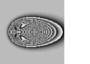
(a)                                                      (b)

Figure 1: (a) Synthetic phase surface generated via eq. (26); (b) wrapped phase pattern: principal phase values span the interval from $-\pi$ (black pixels) to $+\pi$ (white pixels).

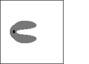
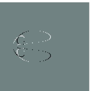
(a)                                                      (b)

Figure 2: (a) Degree of undersampling of the phase field depicted in fig. 1: gray pixels represent locations where the absolute phase gradient differs from its estimate (wrapping of the principal phase gradient) by one $2\pi$-cycle, black pixels represent locations where the difference is 2 cycles; (b) residue map: white pixels are positive residues ($I=1$), black pixels are negative residues ($I=-1$), gray pixels correspond to irrotational locations ($I=0$).

Figure 3: Unwrapped phase reconstructed by the proposed algorithm from the wrapped phase field shown in fig. 1-(b).

Figure 4: Unwrapped phase reconstructed by the LMS algorithm from the wrapped phase field shown in fig. 1-(b).

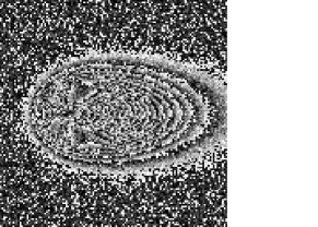
(a)                                                      (b)

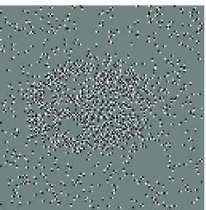
(c)

Figure 5: (a) Same synthetic surface as in fig. 1, with added Gaussian noise with unit variance; (b) principal phase pattern; (c) residue map.

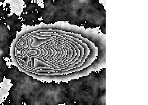
(a)                                                      (b)

Figure 6: (a) Unwrapped surface reconstructed by the proposed algorithm from the wrapped phase field shown in fig. 5-(b); (b) principal phase pattern obtained by re-wrapping the solution depicted in (a).

Appendix A Appendix: Derivatives of the internal energy

We report here the expressions of the derivatives of the internal energy in the Mean-field approximation.

One easily finds that:

$${\partial U\over\partial Q_{x}(x,y)}=4$$

$${\partial U\over\partial Q_{y}(x,y)}=4,$$ (27)

$${\partial U\over\partial m_{x}(x,y)} = -2m_{x}(x-1,y)+{1\over\pi}\left[A_{x}(x,y)-A_{x}(x-1,y)\right]+$$ (28)

$$-2m_{x}(x+1,y)+{1\over\pi}\left[A_{x}(x,y)-A_{x}(x+1,y)\right]+$$

$$-2m_{x}(x,y-1)+{1\over\pi}\left[A_{x}(x,y)-A_{x}(x,y-1)\right]+$$

$$-2m_{x}(x,y+1)+{1\over\pi}\left[A_{x}(x,y)-A_{x}(x,y+1)\right].$$

$${\partial U\over\partial m_{y}(x,y)} = -2m_{y}(x,y-1)+{1\over\pi}\left[A_{y}(x,y)-A_{y}(x,y-1)\right]+$$ (29)

$$-2m_{y}(x,y+1)+{1\over\pi}\left[A_{y}(x,y)-A_{y}(x,y+1)\right]+$$

$$-2m_{y}(x+1,y)+{1\over\pi}\left[A_{y}(x,y)-A_{y}(x+1,y)\right]+$$

$$-2m_{y}(x-1,y)+{1\over\pi}\left[A_{y}(x,y)-A_{y}(x-1,y)\right].$$

References

- [1] A. V. Oppenheim, R. W. Schafer, Digital Signal processing, Prentice-Hall, Englewood Cliffs, N.J., 1975.
- [2] H. P. Hjalmarson, L. A. Romero, D. C. Ghiglia, E. D. Jones, C. B. Norris, Phys. Rev. B 32, 4300 (1985).
- [3] S. Nakadate, H. Saito, Applied Optics 24, 2172 (1985).
- [4] D. L. Fried, J. Opt. Soc. Am. 67, 370 (1977).
- [5] N. H. Ching, D Rosenfeld, M. Braun, IEEE Trans. Im. Proc. 1, 355 (1992).
- [6] H. A. Zebker, R. M. Goldstein, J. Geophis. Res. 91, (B5), 4993 (1986).
- [7] J. Hadamard, “Sur les problémes aux dérivées partielles et leur signification physique”, Princeton University Bulletin 13 (1902).
- [8] S. Geman, D. Geman, IEEE Trans. Pattern Anal. Mach. Intell. 6, 721 (1984).
- [9] B. Gidas, IEEE Trans. Pattern Anal. Mach. Intell. 11, 164 (1989).
- [10] J. Zhang, IEEE Trans. Signal Process. 40, 2570 (1992).
- [11] K. Tanaka, T. Morita, Phys. Lett. A 203, 122 (1995).
- [12] T. Morita, K. Tanaka, Physica A 223, 244 (1996).
- [13] J. Ray, R. W. Harris, Phys. Rev. E 55, 5270 (1997).
- [14] L. Guerriero, G. Nico, G. Pasquariello, S. Stramaglia, Applied Optics 37, 3053 (1998).
- [15] S. Stramaglia, L. Guerriero, G. Pasquariello, N. Veneziani, Applied Optics 38, 1377 (1999).
- [16] D. C. Ghiglia, M. D. Pritt, Two-Dimensional Phase Unwrapping. Theory, Algorithms, and Software, John Wiley & Sons, New York, (1998).
- [17] D. C. Ghiglia, J. A. Romero, J. Opt. Soc. Am. A 11, 107–117, 1994.
- [18] G. Parisi, Statistical Field Theory, Addison-Wesley, Reading MA, (1988).
- [19] For a review on Mean-Field Annealing methods, see e.g. A. L. Yuille, J. J. Kosowsky, Neural Computation 6, 341 (1994).