On the Interplay of Disorder and Correlations

Abstract

I address here the question of the mutual interplay of strong correlations and disorder in the system. I consider random version of the Hubbard model. Diagonal randomness is introduced via random on-site energies and treated by the coherent potential approximation. Strong, short ranged, electron - electron interactions are described by the slave boson technique and found to induce additional disorder in the system. As an example I calculate the density of states of the random interacting binary alloy and compare it with that for non-interacting system. PACS numbers: 71.10.Fd, 71.23.-k, 71.55.Ak.

1 INTRODUCTION

The list of materials in which carriers are strongly interacting with each other and scatter by random impurities is quite long. It comprises inter alia high temperature superconducting oxides $\sevenrm^{\hbox{\immediate{\bf?}}}$ and various heavy fermion alloys .$\sevenrm^{\hbox{\immediate{\bf?}}}$ Two models are usually used to study such system. It is either Hubbard or Anderson model suitably extended to allow for the description of real materials. Here the single band Hubbard model has been used, as it is the simplest model of correlated system. The disorder is introduced into the model by allowing for fluctuations of the local on-site energies $\varepsilon_{i}$. The main purpose of this work is to study the interplay of disorder and correlations in the Hubbard model. I shall present analytical and numerical calculations indicating that correlations induce additional disorder in the system. Mutatis mutandis disorder in the system affects the parameters of the Mott-Hubbard metal-insulator transition. In the recent studies of weakly interacting disordered systems it has been found that due to disorder the interactions scale to strong coupling limit .$\sevenrm^{\hbox{\immediate{\bf?}}}$ Here to treat many particle aspect of the problem we use the slave boson technique, which is known to be qualitatively valid for all strength of interaction. In particular this method reproduces the results of the Gutzwiller approximation at the saddle-point level .$\sevenrm^{\hbox{\immediate{\bf?}}}$

2 THE MODEL AND APPROACH

We start here with random version of the Hubbard model

$$H=\sum_{ij\sigma}t_{ij}c_{i\sigma}^{+}c_{j\sigma}+\sum_{i\sigma}(\varepsilon_{i}-\mu)c_{i\sigma}^{+}c_{i\sigma}+U\sum_{i}n_{i\uparrow}n_{i\downarrow}\,.$$ (1)

The meaning of symbols is standard. The first term describes the hopping of carriers through the crystal specified by lattice sites $i$, $j$. $\varepsilon_{i}$ denotes the fluctuating site energy - it introduces disorder into the model. $U$ is the repulsion between two opposite spin electrons occupying the same site. In the slave boson technique$\sevenrm^{\hbox{\immediate{\bf?}}}$ one introduces 4 auxiliary boson fields: $\hat{e}_{i}$, $\hat{s}_{i\sigma}$, $\hat{d}_{i}$ such that $\hat{e}^{+}_{i}\hat{e}_{i}$, $\hat{s}^{+}_{i\sigma}\hat{s}_{i\sigma}$, $\hat{d}^{+}_{i}\hat{d}_{i}$ project onto the empty, singly occupied by $\sigma$ and doubly occupied site $i$. The Hamiltonian (1) is in this enlarged Hilbert space written as

$$H=\sum_{ij\sigma}t_{ij}\hat{z}^{+}_{i\sigma}\hat{z}_{j\sigma}c^{+}_{i\sigma}c_{j\sigma}+U\sum_{i}\hat{d}^{+}_{i}\hat{d}_{i}+\sum_{i\sigma}(\varepsilon_{i}-\mu)c^{+}_{i\sigma}c_{i\sigma}\,,$$ (2)

where $\hat{z}_{i\sigma}=(\hat{1}-\hat{d}^{+}_{i}\hat{d}_{i}-\hat{s}^{+}_{i\sigma}\hat{s}_{i\sigma})^{-1/2}(\hat{e}^{+}_{i}\hat{s}_{i\sigma}+\hat{s}^{+}_{i-\sigma}\hat{d}_{i})\cdot(\hat{1}-\hat{e}^{+}_{i}\hat{e}_{i}-\hat{s}^{+}_{i-\sigma}\hat{s}_{i-\sigma})^{-1/2}$. Equation (2) is strictly equivalent to (1), when the constraints

$$\hat{e}^{+}_{i}\hat{e}_{i}+\sum_{\sigma}\hat{s}^{+}_{i\sigma}\hat{s}_{i\sigma}+\hat{d}^{+}_{i}\hat{d}_{i}=1$$

$$c^{+}_{i\sigma}c_{i\sigma}=\hat{p}^{+}_{i\sigma}\hat{p}_{i\sigma}+\hat{d}^{+}_{i}\hat{d}_{i};~{}~{}~{}~{}~{}~{}\sigma=\uparrow,\downarrow$$ (3)

are fulfilled. In disordered system and at $T$ = 0 K, the mean field approach to slave bosons can be formulated by suitably generalizing the clean limit. One introduces the constraints into Hamiltonian with help of Langrange multipliers $\lambda_{i}^{(1)}$ and $\lambda_{i\sigma}^{(2)}$ and replaces boson operators $\hat{e}_{i}$, $\hat{s}_{i\sigma}$, $\hat{d}_{i}$ by classical, site dependent, amplitudes $e_{i}$, $s_{i\sigma}$, $d_{i}$. These amplitudes are calculated from the, configuration dependent, ground state energy $E_{GS}=\langle H\rangle$ by minimizing $E_{GS}$ with respect to all seven parameters $e_{i}$, $s_{i\sigma}$, $d_{i}$, $\lambda_{i}^{(1)}$, $\lambda_{i\sigma}^{(2)}$. As a result one gets three constraints: $e_{i}^{2}+\sum_{\sigma}s_{i\sigma}^{2}+d_{i}^{2}=1$, $\langle c_{i\sigma}^{+}c_{i\sigma}\rangle=s_{i\sigma}^{2}+d_{i}^{2}$ and four additional equations which read

$$\lambda_{i}^{(1)}e_{i}=-{\frac{1}{\xi_{i}}}{\frac{\partial\xi_{i}}{\partial e_{i}}}\,{\rm Re}\left(\sum_{j\sigma}t_{ij}\xi_{i}\langle c_{i\sigma}^{+}c_{j\sigma}\rangle\xi_{i}\right)$$

$$(\lambda_{i}^{(1)}-\lambda_{i\sigma}^{(2)})s_{i\sigma}=-{\frac{1}{\xi_{i}}}{\frac{\partial\xi_{i}}{\partial s_{i\sigma}}}\,{\rm Re}\left(\sum_{j}t_{ij}\xi_{i}\langle c_{i\sigma}^{+}c_{j\sigma}\rangle\xi_{i}\right)$$

$$\left(U+\lambda_{i}^{(1)}-\sum_{\sigma}\lambda_{i\sigma}^{(2)}\right)d_{i}=-{\frac{1}{\xi_{i}}}{\frac{\partial\xi_{i}}{\partial d_{i}}}\left({\rm Re}\sum_{j\sigma}t_{ij}\xi_{i}\langle c_{i\sigma}^{+}c_{j\sigma}\rangle\xi_{j}\right)$$ (4)

where $\xi_{i}=(1-d_{i}^{2}-s_{i\sigma}^{2})^{-1/2}(e_{i}s_{i\sigma}+s_{i-\sigma}d_{i})(1-e_{i}^{2}-s_{i-\sigma}^{2})^{-1/2}$.

The important next step is connected with calculation of $\langle c_{i\sigma}^{+}c_{i\sigma}\rangle$ and $E_{i\sigma}=\sum_{j}t_{ij}\xi_{i}\langle c_{i\sigma}^{+}c_{j\sigma}\rangle\xi_{i}$ in the presence of disorder. In principle these quantities do depend on the particular distribution of all impurities (i.e. distribution of site energies $\varepsilon_{i}$). We shall calculate them from the corresponding Green’s function. We use a version$\sevenrm^{\hbox{\immediate{\bf?}}}$ of the coherent potential approximation (CPA) to calculate (averaged and conditionally averaged) Green’s functions. To this end we rewrite the mean field Hamiltonian in the form

$$\tilde{H}=\sum_{ij\sigma}t_{ij}\xi_{i}\xi_{j}c_{i\sigma}^{+}c_{j\sigma}+\sum_{i\sigma}(\varepsilon_{i}-\mu+\lambda_{i\sigma}^{(2)})c_{i\sigma}^{+}c_{i\sigma}+{\rm const}\,.$$ (5)

Note, that Hamiltonian (5) contains not only the site dependent parameters $\varepsilon_{i}$ but due to correlations there appear also $\lambda_{i\sigma}^{(2)}$ which are the additional source of, diagonal and spin dependent, disorder. Besides that, the parameters $\xi_{i}$, $\xi_{j}$ which vary from site to site make effective hopings $\tilde{t}_{ij}=t_{ij}\xi_{i}\xi_{j}$ random quantities. This off-diagonal (in Wannier space) disorder is particularly important. Fortunately multiplicative dependence of effective hopping on the kind of atoms at sites $i$ and $j$ is easy to handle within CPA.

The procedure is standard$\sevenrm^{\hbox{\immediate{\bf?}}}$ and one gets the following equation for the density of states in paramagnetic phase

$$D(\varepsilon)=-{\frac{1}{\pi}}\,{\rm Im}\langle{\frac{\xi_{i}^{2}F[\Sigma(\varepsilon^{+})]}{1-\left[\Sigma(\varepsilon^{+})-(\varepsilon-\varepsilon_{i}+\mu-\lambda_{i}^{(2)})/\xi_{i}^{2}\right]\,F[\Sigma(\varepsilon)]}}\rangle_{{\rm imp}}$$ (6)

and the coherent potential $\Sigma(\varepsilon)$ is determined as a solution of equations

$$\langle{\frac{\Sigma(z)-(z-\varepsilon_{i}+\mu-\lambda_{i}^{(2)})/\xi_{i}^{2}}{1-\left[\Sigma(z)-(z-\varepsilon_{i}+\mu-\lambda_{i}^{(2)})/\xi_{i}^{2}\right]\,F[\Sigma(z)]}}\rangle_{{\rm imp}}=0$$

$$F[\Sigma(z)]={\frac{1}{N}}\sum_{\vec{k}}{\frac{1}{\Sigma(z)-\varepsilon(\vec{k})}}={\frac{1}{N}}\sum_{\vec{k}}\,\bar{G}_{\vec{k}}(z)$$ (7)

Here $\langle\cdots\rangle_{{\rm imp}}$ means averaging over disorder and $\varepsilon(\vec{k})={\frac{1}{N}}\sum_{ij}t_{ij}\,e^{-i\vec{k}(\vec{R}_{i}-\vec{R}_{j})}$ is electron spectrum in host (clean) material.

To solve equations (4) one still has to calculate the quantities $E_{i\sigma}=\sum_{j}t_{ij}\xi_{i}\langle c_{i\sigma}^{+}c_{j\sigma}\rangle\xi_{j}$ , which in general depend on the configuration of all impurities in the system. They can be calculated from the knowledge of the CPA Green’s functions in the following way. We assume that site $i$ is described by actual parameters i.e. $\varepsilon_{i}$, $\lambda_{i\sigma}^{(2)}$, $\xi_{i}$, while all other sites in the system are replaced by effective ones described by the coherent potential $\Sigma(z)$ and the Green’s functions $\bar{G}(z)$. Then it is easy to find that e.g.

$$E_{i\sigma}=\int d\omega{\frac{1}{e^{\beta\omega}+1}}\sum_{j}t_{ij}\left(-{\frac{1}{\pi}}\right)\,{\rm Im}\tilde{G}_{ij\sigma}(\omega+i0)$$ (8)

and $\sevenrm^{\hbox{\immediate{\bf?}}}$

$$\tilde{G}_{ij\sigma}(z)=\bar{G}_{ij\sigma}(z){\frac{1}{1-\tilde{\varepsilon}_{i\sigma}(z)\bar{G}_{ii\sigma}(z)}}$$ (9)

Here $\tilde{\varepsilon}_{i\sigma}(z)=(z-\varepsilon_{i}+\mu-\lambda_{i\sigma}^{(2)})/\xi_{i}^{2}$, and by definition $\bar{G}_{ii\sigma}(z)\equiv F[\Sigma(z)]$ and $\bar{G}_{ij\sigma}(z)=\frac{1}{N}\sum_{\vec{k}}\bar{G}_{\vec{k}}(z)e^{i\vec{k}(\vec{R}_{i}-\vec{R}_{j})}$  This closes the system of equations to be solved in a self-consistent manner. In the next section we show numerical calculations of the effect of correlations on the density of states in disordered alloy.

3 NUMERICAL RESULTS AND DISCUSSION

For the purpose of numerical illustration of the general approach sketched in previous section we calculate here the density of states (DOS) of perfect interacting, random noninteracting and random interacting systems. For the purpose of numerical analysis we shall assume $U=\infty$ limit and bcc crystal structure, which leads to the following canonical tight-binding spectrum of noninteracting carriers in clean material

$$\varepsilon_{\vec{k}}=-8t\cos(k_{x}a)\cos(k_{y}a)\cos(k_{z}a).$$ (10)

Using t=0.0625$eV$ leads to the noninteracting system bandwidth $W=1eV$. In the following all energies and frequencies are expressed in $eV$. The density of states corresponding to this spectrum is well known. It possesses Van Hove singularity in the middle of the band, which extends from $-8t$ to $+8t$. The spectrum $\varepsilon_{\vec{k}}$ of a clean but interacting system in the $U=\infty$ limit is replaced by $\xi^{2}\varepsilon_{\vec{k}}-\lambda^{(2)}$. The corresponding density of states is thus of the same form but placed in the energy window $[-8t(1-n)-\lambda^{(2)},+8t(1-n)-\lambda^{(2)}]$ and scaled by the factor $(1-n)^{-1}$. Note that in this $U=\infty$ limit the upper Hubbard band is pushed to infinity and not visible.

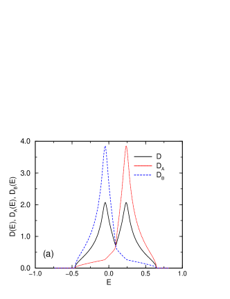
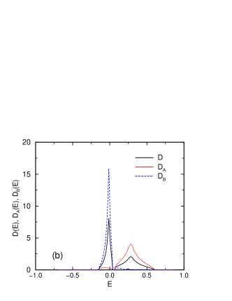
Fig. 1: Comparison of the DOS of (a) disordered noninteracting $A_{1-x}B_{x}$ alloy with $x=0.5$, $\varepsilon_{A}=0$, $\varepsilon_{B}=-0.3eV$ with that calculated for the same alloy but with interacting carriers (b). Carrier density $n=0.4$.

The changes of the spectrum due to correlations in disordered $A_{1-x}B_{x}$ alloy are illustrated in figure (1) where we show the averaged $D(E)$ and conditionally averaged densities of states $D_{A}(E)$ and $D_{B}(E)$  ($x=0.5$, $\varepsilon_{A}=0,\varepsilon_{B}=-0.3eV$) without (Fig. 2a) and with (Fig. 2b) electron correlations. The carrier concentration $n=0.4$. Noninteracting alloy DOS is symmetric. We observe strong asymmetry, the opening of the real gap in the spectrum of interacting carriers and the appreciable increase of the density of states at the fermi level (taken as E=0 in the figure).

In conclusion, we have shown that interplay of disorder and correlations leads to strong renormalisation of the electron spectrum. Let us stress that all other properties of such systems will also be strongly affected by interaction induced disorder. The calculations of dc and ac transport properties are in progress.

References

• [1] K. Ishida et al., J.Phys.Soc. Jpn. 62, 2803 (1993); Gang Xiao et al., Phys. Rev. B42, 8752 (1990); B.Beschoten et al., Phys. Rev. Lett. 77, 1837 (1996).
• [2] B. Andraka and G. R. Stewart, Phys. Rev. B47, 3208 (1993); O. O. Bernal et al., Phys. Rev. Lett. 75, 2023 (1995); B. Maple et al., J. Low Temp. Phys. 99, 223 (1995).
• [3] D. Belitz and T. R. Kirkpatrick, Rev. Mod. Physics 66, 261 (1994).
• [4] W. F. Brinkman and T. M. Rice, Phys. Rev. B 2, 4302 (1970).
• [5] G. Kotliar and A. E. Ruckenstein, Phys. Rev. Lett. 57 , 1362 (1986).
• [6] K. I. Wysokiński, J. Phys. C11, 291 (1978).
• [7] E. N. Economou, Green’s Function in Quantum Physics , Springer Verlag, Berlin 1983, ch. 6.