EFFECTIVE POTENTIAL APPROACH TO QUANTUM DISSIPATION IN CONDENSED MATTER SYSTEMS

Abstract

The effects of dissipation on the thermodynamic properties of nonlinear quantum systems are approached by the path-integral method in order to construct approximate classical-like formulas for evaluating thermal averages of thermodynamic quantities. Explicit calculations are presented for one-particle and many-body systems. The effects of the dissipation mechanism on the phase diagram of two-dimensional Josephson arrays is discussed.

1 Introduction

The usefulness of the improved [1] effective potential approach, [2] has been proven by several applications to condensed matter systems. However, open systems were not immediately treated and previous studies were confined to obtain a classical-like expression for the free energy. [3, 4]

In fact, the effective-potential method, also called pure-quantum self-consistent harmonic approximation (PQSCHA) after its generalization to phase-space Hamiltonians, [5, 6] is able [7] to give the density matrix of a nonlinear system interacting with a dissipation bath through the Caldeira-Leggett (CL) model. [8] For a better understanding of the method let us first consider one single degree of freedom. In the general case the CL model starts from the Hamiltonian

$$\hat{H}={\hat{p}^{2}\over 2m}+V(\hat{q})+{1\over 2}\sum_{i}\bigg{\{}{\hat{p}_{i}^{2}\over m_{i}}+m_{i}\omega_{i}^{2}\Big{[}\hat{q}_{i}-F_{i}(\hat{q})\Big{]}^{2}\bigg{\}}~{},$$ (1)

where $(\hat{p},\hat{q})$ and $(\hat{p}_{i},\hat{q}_{i})$ are the momenta and coordinates of the system and of an environment (or bath) of harmonic oscillators. When $F_{i}(\hat{q})=\hat{q}$ the dissipation is said to be linear and we will restrict ourselves to this case in the following. The bath coordinates can be integrated out exactly from the corresponding path integral and the CL Euclidean action is obtained in the form:

$$S[q(u)]=\!\int_{0}^{\beta}\!\!\!du\left[{m\over 2}\dot{q}^{2}(u){+}V\big{(}q(u)\big{)}\right]+\!\int_{0}^{\beta}\!{du\over 2}\!\int_{0}^{\beta}\!\!\!\!du^{\prime}\,k(u{-}u^{\prime})\,q(u)\,q(u^{\prime})\,.$$ (2)

To make contact with the classical concept of dissipation, one may take the classical counterpart of Eq. (1) and get the Langevin equation of motion:

$$m\ddot{q}+m\int_{0}^{\infty}\!\!dt^{\prime}\,\gamma(t^{\prime})\,\dot{q}(t{-}t^{\prime})+V^{\prime}(q)=0~{};$$

then the Laplace transform $\gamma(z)$ of the damping function $\gamma(t)$, as expressed in terms of the spectral density of the environmental coupling, [3] can be related to the Matsubara components of the damping kernel $k(u)$ ($\nu_{n}=2\pi{n}/\beta$) :

$$k(u)\equiv m\beta^{-1}~{}{\textstyle{\sum}_{n}}~{}e^{i\nu_{n}u}\,k_{n}~{},~{}~{}~{}~{}~{}~{}~{}~{}~{}~{}~{}k_{n}=|\nu_{n}|\,\gamma\big{(}z{=}|\nu_{n}|\big{)}~{},$$ (3)

We will consider two cases:

$${\rm Ohmic:~{}~{}~{}~{}~{}~{}} \gamma(t)=\gamma\,\delta(t-0)~{},~{}~{}~{}~{}~{}~{}~{}\,\gamma(z)=\gamma~{},$$

$${\rm Drude:~{}~{}~{}~{}~{}~{}} \gamma(t)=\gamma\,\omega_{\rm{D}}\,e^{-\omega_{\rm{D}}t}~{},~{}~{}~{}~{}~{}~{}\gamma(z)={\gamma\,\omega_{\rm{D}}/(\omega_{\rm{D}}+z)}~{},$$

where the dissipation strength $\gamma$ and the bath bandwidth $\omega_{\rm{D}}$ characterize the environmental coupling; $\omega_{\rm{D}}\to\infty$ gives the Ohmic (or Markovian) case. In order to interpolate between different regimes and to take into account memory effects we can also assume:

$$\gamma(z)\propto z^{s}~{},$$ (4)

with $-1<s<1$ and $s>0$ ($s<0$) is said the super- (sub-) Ohmic case.

2 Effective potential in presence of dissipation

The PQSCHA approximation consists in taking as trial action $S_{0}$, the most general quadratic functional with the same linear dissipation of $S$, namely,

$$S_{0}[q(u)] = \int_{0}^{\beta}du\left[{m\over 2}\dot{q}^{2}(u)+w+m\omega^{2}\,\big{(}q(u){-}\bar{q}\big{)}^{2}\right]$$ (5)

$$\hskip 56.9055pt+\!\int_{0}^{\beta}\!{du\over 2}\!\int_{0}^{\beta}\!\!\!\!du^{\prime}\,k(u{-}u^{\prime})\,q(u)\,q(u^{\prime})\,.$$

The quantity $\bar{q}=\beta^{-1}\int{q(u)}\,du$ is the average point of paths and

$$w=w(\bar{q})~{},~{}~{}~{}~{}~{}~{}~{}\omega^{2}=\omega^{2}(\bar{q})~{},$$ (6)

are parameters to be determined by minimizing the right-hand side of the Feynman inequality,

$$F\leq{F_{0}}+\beta^{-1}\langle S-S_{0}\rangle_{S_{0}}~{}.$$ (7)

For any observable $\hat{\cal O}(\hat{p},\hat{q})$ the $S_{0}$-average can be expressed [6, 7] in terms of its Weyl symbol [9] ${\cal O}(p,q)$. As final result we obtain the classical-like form

$$\langle\hat{{\cal O}}\rangle=\frac{1}{{\cal Z}_{0}}\sqrt{m\over{2\pi\hbar^{2}\beta}}\int\,d\bar{q}~{}\big{\langle}\!\big{\langle}{\cal O}(p,\bar{q}+\xi)\big{\rangle}\!\big{\rangle}~{}e^{-\beta\,V_{\rm eff}(\bar{q})}~{},$$ (8)

where $\langle\!\langle{\cdots}\rangle\!\rangle$ is a Gaussian average operating over $p$ and $\xi$ with moments

$$\langle\!\langle{\xi^{2}}\rangle\!\rangle\equiv\alpha(\bar{q}) = {2\over\beta m}~{}\sum\limits_{n=1}^{\infty}{1\over\nu_{n}^{2}{+}\omega^{2}(\bar{q}){+}k_{n}}~{}~{}\xrightarrow[k\to{0}]{~{}}~{}{1\over 2m\omega}\Big{(}\coth f{-}{1\over f}\Big{)}~{},$$ (9)

$$\langle\!\langle{p^{2}}\rangle\!\rangle\equiv\lambda(\bar{q}) = {m\over\beta}\,\sum\limits_{n=-\infty}^{\infty}{\omega^{2}(\bar{q})+k_{n}\over\nu_{n}^{2}{+}\omega^{2}(\bar{q}){+}k_{n}}~{}~{}\xrightarrow[k\to{0}]{~{}}~{}{m\omega\over 2}\coth f~{},$$ (10)

where $f\equiv\beta\omega/2$. The effective potential is defined as $V_{\rm eff}(\bar{q})\equiv w(\bar{q})+\sigma(\bar{q})$ , with

$$\sigma(\bar{q})={1\over\beta}\sum_{n=1}^{\infty}\ln\,{\nu_{n}^{2}{+}\omega^{2}(\bar{q}){+}k_{n}\over\nu_{n}^{2}}~{}~{}\xrightarrow[k\to{0}]{~{}}~{}{1\over\beta}\,\ln{\sinh f\over f}~{}.$$ (11)

The r.h.s. of Eqs. (9-11) show that the well known non-dissipative limits are recovered for ${k\to{0}}$. The variational parameters can be self-consistently calculated and the explicit expressions are the following

$$w(\bar{q})=\big{\langle}\!\big{\langle}V(\bar{q}+\xi)\big{\rangle}\!\big{\rangle}-{\textstyle\frac{1}{2}}m\omega^{2}\alpha~{},\hskip 28.45274ptm\,\omega^{2}(\bar{q})=\big{\langle}\!\big{\langle}V^{\prime\prime}(\bar{q}+\xi)\big{\rangle}\!\big{\rangle}~{}.$$ (12)

3 Applications

In order to understand how this approximation scheme works, let us take first a very simple system: one particle in a double-well potential with Ohmic dissipation. A typical result for this system is shown in Fig. 1: the dissipation quenches the quantum fluctuations of the coordinate. However, it must be noted from Eq.(10) that those of the momentum are infinite.

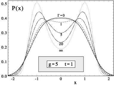
Figure 1: Configuration density $P(x)=\langle\delta(\hat{x}-x)\rangle$ of the double-well quartic potential for the fixed coupling $g=5$, the reduced temperature $t=1$, and different values of the Ohmic damping parameter $\Gamma=\gamma/\omega_{0}$, being $\omega_{0}$ the characteristic frequency of the system. The filled circles are the exact result for $\Gamma=0$; the dotted curve at $\Gamma=\infty$ corresponds to the classical limit.

Let us now turn to the many-body case. The first application is a quantum $\varphi^{4}$-chain of particles with Drude-like dissipation: [10] the undamped system is described by the following action

$$S_{\varphi^{4}}={3\over{2Q}}\int_{0}^{\beta}du\,a\,\sum_{i}\left[{\dot{q}_{i}^{2}\over 2}+{(q_{i}-q_{i-1})^{2}\over 2a^{2}}+{\Omega^{2}\over 8}\big{(}1-q_{i}^{2}\big{)}^{2}\right]~{},$$ (13)

where $a$ is the chain spacing, $\Omega$ is the gap of the bare dispersion relation, and $Q$ is the quantum coupling. The classical continuum model supports kink excitations of characteristic width $\Omega^{-1}$ and static energy $\varepsilon_{\rm{K}}=\Omega/Q$. This energy is used as the energy scale in defining the reduced temperature $t\equiv(\beta\varepsilon_{\rm{K}})^{-1}$. We also use the kink length in lattice units $R\equiv(a\Omega)^{-1}$ ($R\to\infty$ in the continuum limit). We assume uncorrelated identical CL baths for each degree of freedom, and use the low-coupling approximation [6] (LCA) in order to deal with the effective potential. The partition function turns out to be written as

$${\cal{Z}} = ({3t\over 4\pi RQ^{2}})^{N\over 2}\!\!\!\int\!d^{N}\!q\;e^{-\beta V_{\rm eff}}~{},$$ (14)

$$\beta V_{\rm eff} = \frac{3}{2Rt}{\sum}_{i}\left[{R^{2}\over 2}(q_{i}-q_{i-1})^{2}+v_{\rm eff}(q_{i})\right]~{},$$ (15)

$$v_{\rm eff}(q) = {1\over 8}\big{(}1-3D-q^{2}\big{)}^{2}+{3\over 4}D^{2}+{Rt\over N}{\sum}_{k}\sigma_{k}~{}.$$ (16)

The renormalization parameter $D=D(t;Q,R;\gamma,\omega_{\rm{D}})$ generalizes Eq. (9) and is the solution of the self-consistent equations:

$$D = {4Rt\over 3N}{\sum}_{k}{\sum}_{n}{\Omega^{2}\over\nu_{n}^{2}+\omega_{k}^{2}+k_{n}},$$ (17)

$$\omega_{k}^{2}(t) = \Omega^{2}\big{[}(1-3D)+4R^{2}\sin^{2}(ka/2)\big{]}~{},$$ (18)

where $k_{n}=\gamma\omega_{\rm{D}}\,\nu_{n}/(\omega_{\rm{D}}+\nu_{n})$ and here $\nu_{n}/\Omega=2\pi{n}t/Q$.

Again, we observe that the fluctuations of coordinate-dependent observables are quenched by increasing the dissipation strength $\gamma$, while those of momentum-dependent ones are enhanced due to the momentum exchanges with the environment. The result of these opposite behaviors is a non-trivial dependence on dissipation of “mixed” quantities like the specific heat as is shown in Fig. 2 .

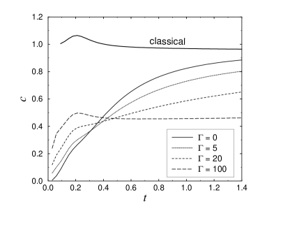
Figure 2: Total specific heat $c(t)$ and the kinetic and interaction parts of the specific heat, namely $c_{{}_{\rm{K}}}(t)=\partial_{t}\langle\hat{K}\rangle$ and $c_{{}_{\rm{V}}}(t)=\partial_{t}\langle\hat{V}\rangle$ vs. reduced temperature $t$, for different values of the damping strength $\Gamma=\gamma/\Omega$. Note that for $\Gamma\to\infty$, $c(t)$ tends to $c_{\rm{cl}}-1/2$: this behavior can be explained by observing that, in the strong damping limit, $c_{{}_{\rm{K}}}(t)\to{0}$.

The last system we consider is the dissipative quantum XY model. Much interest in such system is due to its close relation with 2D granular superconductors and Josephson junction arrays (JJA). In the last 15 years much attention has been devoted to the theoretical and experimental study [11] of the phase ordering in JJA and of how it is influenced by the environmental coupling. The undamped system is described by the action

$$S_{\rm JJA}=\int_{0}^{\beta}du\bigg{\{}\frac{1}{2}\sum_{ij}{\dot{\phi}_{i}(u)\frac{C_{ij}}{4e^{2}}\dot{\phi}_{j}(u)}-J\sum_{<ij>}\cos[\phi_{i}(u)-\phi_{j}(u)]\bigg{\}}~{},$$ (19)

where $\phi_{i}$ is the superconducting phase of the $i$-th island, ${<}ij{>}$ restricts the sum over nearest-neighbor bonds, $J$ is the Josephson coupling, $C_{ij}=(C_{0}+4C_{1})\delta_{ij}-C_{1}\delta_{ij}^{({\rm{nn}})}$, $C_{0}$ and $C_{1}$ are the self and mutual capacitance between superconducting islands and $\delta_{ij}^{({\rm{nn}})}=1$ for nearest neighbors, zero otherwise.

From Eq. (19) two contributions to the energy in this system can be observed: the kinetic one, due to the charging energy between islands ($E_{\rm{c}}=q^{2}/2C$, $q=2e$), and the potential energy, due to the Josephson coupling in the superconducting junctions. When $E_{\rm{c}}{\ll}J$, the charges on each island fluctuate independently from the phases $\phi_{i}$ : the latter have then a classical XY behavior and the associated Berezinskii-Kosterlitz-Thouless (BKT) phase transition takes place at temperature $T^{\rm(cl)}_{{}_{\rm{BKT}}}\sim{0.892}\,J$. In the opposite limit, the energy cost to transfer charges between neighboring islands is too high, so the charges tend to be localized and the phase ordering tends to be suppressed.

In this scenario dissipation is supposed to have an important role. The environmental interaction tends to suppress the quantum fluctuations [12] of $\phi_{i}$ and to restore an almost classical BKT phase transition. Nevertheless, it is not clear which is the physical mechanism of the dissipation. For the single Josephson junction with Ohmic dissipation the classical “resistively and capacitively shunted junction” (RCSJ) model is recovered [12], but in the case of many degrees of freedom the environmental interaction is much more complicated, e.g. non-exponential memory effects and then non-Ohmic damping can appear. The dissipation model we assume consists in independent environmental baths, one for each junction (or bond). The dissipative part of the action is

$$S_{\rm D}={\textstyle\frac{1}{2}}\,{\sum}_{n}\,{{}^{t}\boldsymbol{\phi}_{n}}\boldsymbol{K}_{n}\boldsymbol{\phi}_{n}\,,$$ (20)

where the Fourier transform of the CL kernel matrix is given by

$$K_{n,ij}=\frac{\gamma}{2\pi}\,\bigg{(}\frac{|\nu_{n}|}{\omega_{0}}\bigg{)}^{1+s}(4~{}\delta_{ij}-\delta_{ij}^{\rm(nn)})~{},$$ (21)

and $\omega_{0}$ is a characteristic frequency, that we choose as the Debye frequency

$$\omega_{0}\equiv\omega_{\pi,\pi}=4\bigg{(}\frac{q^{2}}{2C_{0}}\frac{J}{1+8\eta}\bigg{)}^{1/2}~{},~{}~{}~{}~{}~{}\eta\equiv\frac{C_{1}}{C_{0}}.$$ (22)

Now it is possible to define the quantum coupling parameter, that measures the “quanticity” of the system as the ratio between the characteristic quantum and classical energy scales $g=\hbar\omega_{0}/J$. The effective potential is calculated using the extension to the many-body case [10] of the scheme of Sec. 2 and, apart from uniform terms, is given by

$$V_{\rm eff}=-J_{\rm{eff}}(T)\sum_{<ij>}\cos(\phi_{i}-\phi_{j})~{},$$ (23)

where $J_{\rm{eff}}(T)=J\,e^{-D_{1}(T)/2}$ and $D_{1}(T)$ is the renormalization parameter that measures the pure-quantum contribution to the fluctuations of the nn relative superconducting phases. The phase diagram of the system is calculated starting from the classical effective potential (23), i.e. by solving $T_{{}_{\rm{BKT}}}=J_{\rm{eff}}(T_{{}_{\rm{BKT}}})\,T^{\rm(cl)}_{{}_{\rm{BKT}}}$ , and is shown in Fig. 3, for different values of the parameters that characterize the dissipation.

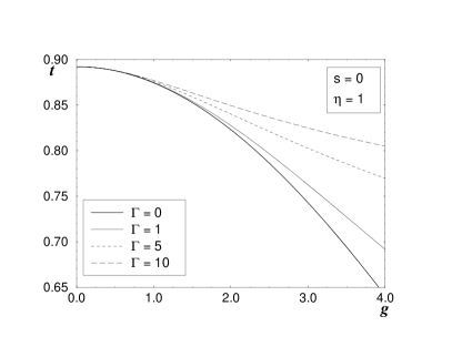
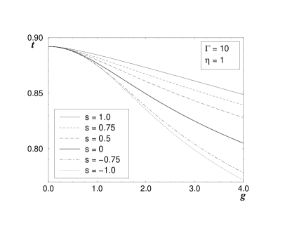
Figure 3: Phase diagram in the $(g,t)$ plane, $t\equiv{T/J}$, for different values of the damping parameters, $\Gamma=\gamma/\omega_{0}$ and $s$. On the left, the case of Ohmic dissipation: the critical temperature $T_{{}_{\rm{BKT}}}$ tends to $T^{\rm(cl)}_{{}_{\rm{BKT}}}$ for increasing damping strength. On the right, for different values of $s$: the cases $s=1$ and $s=-1$ are nondissipative, since they correspond to a variation of the capacitance- and of the frequency spectrum, respectively.

References

• [1] R. Giachetti and V. Tognetti, Phys. Rev. Lett. 55, 912 (1985); Phys. Rev. B 33, 7647 (1986). R. P. Feynman and H. Kleinert, Phys. Rev. A 34, 5080 (1986).
• [2] R.P. Feynman and A.R. Hibbs, Quantum Mechanics and Path Integrals (Mc Graw Hill, New York, 1965).
• [3] U. Weiss, Quantum Dissipative Systems (World Scientific, Singapore, 2nd edition, 1999).
• [4] J.D. Bao, Y.Z. Zhuo, and X. Z. Wu, Phys. Rev. E 52, 5656 (1995).
• [5] A. Cuccoli, V. Tognetti, P. Verrucchi, and R. Vaia, Phys. Rev. A 45, 8418 (1992).
• [6] A. Cuccoli, R. Giachetti, V. Tognetti, R. Vaia and P. Verrucchi, J. Phys.: Condens. Matter 7, 7891 (1995).
• [7] A. Cuccoli, A. Rossi, V. Tognetti, and R. Vaia, Phys. Rev. E 55, 4849 (1997).
• [8] A.O. Caldeira and A.J. Leggett, Ann. of Phys. 149, 374 (1983).
• [9] F.A. Berezin, Sov. Phys. Usp. 23, 763 (1980).
• [10] A. Cuccoli, A. Fubini, V. Tognetti, and R.  Vaia, Phys. Rev. E 60, 231 (1999).
• [11] Proceedings of the ICTP Workshop on Josephson Junction Arrays, edited by H.A. Cerdeira and S.R. Shenoy, Physica B 222(4), 253-406 (1996) and references therein.
• [12] G. Schön and A.D. Zaikin, Phys. Rep. 198, 237 (1990); M. Tinkham, Introdution to superconductivity (McGraw-Hill, New York, 1996).