Generalization properties of finite size polynomial Support Vector Machines

Abstract

The learning properties of finite size polynomial Support Vector Machines are analyzed in the case of realizable classification tasks. The normalization of the high order features acts as a squeezing factor, introducing a strong anisotropy in the patterns distribution in feature space. As a function of the training set size, the corresponding generalization error presents a crossover, more or less abrupt depending on the distribution’s anisotropy and on the task to be learned, between a fast-decreasing and a slowly decreasing regime. This behaviour corresponds to the stepwise decrease found by Dietrich et al. [1] in the thermodynamic limit. The theoretical results are in excellent agreement with the numerical simulations.

I Introduction

In the last decade, the typical properties of neural networks that learn classification tasks from a set of examples have been analyzed using the approach of Statistical Mechanics. In the general setting, the value of a binary output neuron represents whether the input vector, describing a particular pattern, belongs or not to the class to be recognized. Manuscript character recognition and medical diagnosis are examples of such classification problems. The process of inferring the rule underlying the input-output mapping given a set of examples is called learning. The aim is to predict correctly the class of novel data, i.e. to generalize.

In the simplest neural network, the perceptron, the inputs are directly connected to a single output neuron. The output state is given by the sign of the weighted sum of the inputs. Then, learning amounts to determine the weights of the connexions in order to obtain the correct outputs to the training examples. Considering the weights as the components of a vector, the network classifies the input vectors according to whether their projections onto the weight vector are positive or negative. Thus, patterns of different classes are separated by the hyperplane orthogonal to the weight vector. Beyond these linear separations, two different learning schemes have been suggested. Either the input vectors are mapped by linear hidden units to so called internal representations that must be linearly separable by the output neuron, or a more powerful output unit is defined, able to perform more complicated functions than just the weighted sum of its inputs.

The first solution is implemented using feedforward layered neural networks. The classification of the internal representations, performed by the output neuron, corresponds in general to a complicated separation surface in input space. However, the relation between the number of hidden units of a network and the class of rules it can infer is still an open problem. In practice, the number of hidden neurons is either guessed or determined through constructive heuristics.

A solution that uses a more complex output unit, the Support Vector Machine (SVM) [1], has been recently proposed. The input patterns are transformed into high dimensional feature vectors whose components may include the original input together with specific functions of its coordinates selected a priori, with the aim that the learning set be linearly separable in feature space. In that case the learning problem is reduced to that of training a simple perceptron. For example, if the feature space includes all the pairwise products of the input vector, the SVM may implement any classification rule corresponding to a quadratic separating surface in input space. Higher order polynomial SVMs and other types of SVMs may be defined by introducing the corresponding features. A big advantage is that learning a linearly separable rule is a convex optimization problem. The difficulties of having many local minima, that hinder the process of training multilayered neural networks, are thus circumvented. Once the adequate feature space is defined, the SVM selects the particular hyperplane called Maximal Margin (or Maximal Stability) Hyperplane (MMH), which lies at the largest distance to its closest patterns in the training set. These patterns are called Support Vectors (SV). The MMH solution has interesting properties [2]. In particular, the fraction of learning patterns that belong to the SVs provides an upper bound [1] to the generalization error, that is, to the probability of incorrectly classifying a new input. It has been shown [3] that the perceptron weights are a linear combination of the SVs, an interesting property in high dimensional feature spaces, as their number is bounded.

A perceptron can learn with very high probability any set of examples, regardless of the underlying classification rule, provided that their number does not exceed twice its input space dimension [4]. However, this simple rote learning does not capture the rule underlying the classification. As it may arise that the feature space dimension of the SVM is comparable to, or even larger than, the number of available training patterns, we would expect that SVMs have a poor generalization performance. Surprisingly, this seems not to be the case in the applications [5].

Two theoretical papers [6, 7] have recently addressed this interesting question. They determined the typical properties of a family of polynomial SVMs in the limit of large dimensional spaces, reaching completely different results in spite of the seemingly innocuous differences between the models. Both papers consider polynomial SVMs in which the input vectors ${\bf x}\in\mbox{IR}^{N}$ are mapped onto quadratic features $\textstyle\Phi$. More precisely, the normalized mapping ${\mathchoice{{\hbox{\boldmath$\displaystyle\Phi$}}}{{\hbox{\boldmath$\textstyle\Phi$}}}{{\hbox{\boldmath$\scriptstyle\Phi$}}}{{\hbox{\boldmath$\scriptscriptstyle\Phi$}}}}_{n}({\bf x})=({\bf x},x_{1}{\bf x}/\sqrt{N},x_{2}{\bf x}/\sqrt{N},\cdots,x_{N}{\bf x}/\sqrt{N})$ has been considered in [6]. The non-normalized mapping ${\mathchoice{{\hbox{\boldmath$\displaystyle\Phi$}}}{{\hbox{\boldmath$\textstyle\Phi$}}}{{\hbox{\boldmath$\scriptstyle\Phi$}}}{{\hbox{\boldmath$\scriptscriptstyle\Phi$}}}}_{nn}({\bf x})=({\bf x},x_{1}{\bf x},x_{2}{\bf x},\cdots,x_{k}{\bf x})$ has been studied in [7] as a function of $k$, the number of quadratic features. For $k=N$ the dimension of both feature spaces is the same, corresponding to a linear subspace of dimension $N$, and a quadratic subspace of dimension $N^{2}$. The mappings only differ in the distributions of the quadratic components in feature space. Due to the normalization, those of ${\mathchoice{{\hbox{\boldmath$\displaystyle\Phi$}}}{{\hbox{\boldmath$\textstyle\Phi$}}}{{\hbox{\boldmath$\scriptstyle\Phi$}}}{{\hbox{\boldmath$\scriptscriptstyle\Phi$}}}}_{n}$ are squeezed by a normalizing factor $a=1/\sqrt{N}$ with respect to those of ${\mathchoice{{\hbox{\boldmath$\displaystyle\Phi$}}}{{\hbox{\boldmath$\textstyle\Phi$}}}{{\hbox{\boldmath$\scriptstyle\Phi$}}}{{\hbox{\boldmath$\scriptscriptstyle\Phi$}}}}_{nn}$. In the case of learning a linearly separable rule with the non-normalized mapping ${\mathchoice{{\hbox{\boldmath$\displaystyle\Phi$}}}{{\hbox{\boldmath$\textstyle\Phi$}}}{{\hbox{\boldmath$\scriptstyle\Phi$}}}{{\hbox{\boldmath$\scriptscriptstyle\Phi$}}}}_{nn}$, the generalization error at any given learning set size increases dramatically with the number $k$ of quadratic features included [7]. On the contrary, in the case of mapping ${\mathchoice{{\hbox{\boldmath$\displaystyle\Phi$}}}{{\hbox{\boldmath$\textstyle\Phi$}}}{{\hbox{\boldmath$\scriptstyle\Phi$}}}{{\hbox{\boldmath$\scriptscriptstyle\Phi$}}}}_{n}$, the generalization error exhibits an interesting stepwise decrease, also found within the Gibbs learning paradigm in a quadratic feature space [8]. If the number of training patterns scales with $N$, the dimension of the linear subspace, it decreases up to an asymptotic lower bound. If the number of examples scales proportionally to $N^{2}$, it vanishes asymptotically. In particular, if the rule to be inferred is linearly separable in the input space, learning in the feature space with the mapping ${\mathchoice{{\hbox{\boldmath$\displaystyle\Phi$}}}{{\hbox{\boldmath$\textstyle\Phi$}}}{{\hbox{\boldmath$\scriptstyle\Phi$}}}{{\hbox{\boldmath$\scriptscriptstyle\Phi$}}}}_{n}$ is harmless, as the decrease of the generalization error with the number of training patterns presents a slight slow-down with respect to that of a simple perceptron learning in input space.

As this stepwise learning is exclusively related to the fact that the normalizing factor of the quadratic features vanishes in the thermodynamic limit $N\rightarrow\infty$, in the present paper we determine the influence of the normalizing factor on the typical generalization performance of finite size SVMs. To this end, we introduce two parameters, $\sigma$ and $\Delta$, caracterizing the mapping of the $N$-dimensional input patterns onto the feature space. The variance $\sigma$ reflects the width of the high-order features distribution and is related to the normalizing factor $a$. The inflation factor $\Delta$ accounts for the proportion of quadratic features with respect to the input space dimension $N$. Actual quadratic SVMs are caracterized by different values of $\Delta$ and $\sigma$, depending on $N$ and $a$. Keeping $\sigma$ and $\Delta$ fixed in the thermodynamic limit allows us to determine the typical properties of actual SVMs, which have finite compressing factors and inflation ratios.

In fact, the behaviour of the SVMs is the same as that of a simple perceptron learning a training set with patterns drawn from a highly anisotropic probability distribution, such that a macroscopic fraction of components have a different variance from the others. Not surprisingly, we find that the asymptotic behaviour corresponding to both the small and large training set size limits, is the same as the one of the perceptron’s MMH. Only the prefactors depend on the mapping used by the SVM.

As expected, the stepwise learning obtained with the normalized mapping in the thermodynamic limit becomes a crossover. Upon increasing the number of training patterns, the generalization error first present an abrupt decrease, that corresponds to learning the weight components in the linear subspace, followed by a slower decrease corresponding to the learning of the quadratic components. The steepness of the crossover not only depends on $\Delta$ and $\sigma$, but also on the task to be learned. The agreement between our analytic results and numerical simulations is excellent.

The paper is organized as follows: in section II we introduce the model and the main steps of the Statistical Mechanics calculation. Numerical simulation results are compared to the corresponding theoretical predictions in section III. The two regimes of the generalization error and the asymptotic behaviours are discussed in section IV. The conclusion is left to section V.

II The model

We consider the problem of learning a binary classification task from examples with a SVM in polynomial feature spaces. The learning set contains $M$ patterns $({\bf x}^{\mu},\tau^{\mu})$ ($\mu=1,\cdots,M$) where ${\bf x}^{\mu}$ is an input vector in the $N$-dimensional input space, and $\tau^{\mu}\in\{-1,1\}$ is its class. We assume that the components $x_{i}^{\mu}$ ($i=1,\cdots,N$) are independent identically distributed (i.i.d.) random variables drawn from gaussian distributions having zero-mean and unit variance:

$$P({\bf x})=\prod_{i=1}^{N}\frac{1}{\sqrt{2\pi}}\exp\left(-\frac{x_{i}^{2}}{2}\right).$$ (1)

In the following we concentrate on quadratic feature spaces, although our conclusions are more general, and may be applied to higher order polynomial SVMs, as discussed in section IV. The mappings ${\mathchoice{{\hbox{\boldmath$\displaystyle\Phi$}}}{{\hbox{\boldmath$\textstyle\Phi$}}}{{\hbox{\boldmath$\scriptstyle\Phi$}}}{{\hbox{\boldmath$\scriptscriptstyle\Phi$}}}}_{nn}({\bf x})=({\bf x},x_{1}{\bf x},x_{2}{\bf x},\cdots,x_{N}{\bf x})$ and ${\mathchoice{{\hbox{\boldmath$\displaystyle\Phi$}}}{{\hbox{\boldmath$\textstyle\Phi$}}}{{\hbox{\boldmath$\scriptstyle\Phi$}}}{{\hbox{\boldmath$\scriptscriptstyle\Phi$}}}}_{n}({\bf x})=({\bf x},x_{1}{\bf x}/\sqrt{N},x_{2}{\bf x}/\sqrt{N},\cdots,x_{N}{\bf x}/\sqrt{N})$ are particular instances of mappings of the form ${\mathchoice{{\hbox{\boldmath$\displaystyle\Phi$}}}{{\hbox{\boldmath$\textstyle\Phi$}}}{{\hbox{\boldmath$\scriptstyle\Phi$}}}{{\hbox{\boldmath$\scriptscriptstyle\Phi$}}}}({\bf x})=(\phi_{1},\phi_{2},\cdots,\phi_{N},\phi_{11},\phi_{12},\cdots,\phi_{NN})$ where $\phi_{i}=x_{i}$, and $\phi_{ij}=a\,x_{i}x_{j}$, where $a$ is the normalizing factor of the quadratic components: $a=1$ for mapping ${\mathchoice{{\hbox{\boldmath$\displaystyle\Phi$}}}{{\hbox{\boldmath$\textstyle\Phi$}}}{{\hbox{\boldmath$\scriptstyle\Phi$}}}{{\hbox{\boldmath$\scriptscriptstyle\Phi$}}}}_{nn}$ and $a=1/\sqrt{N}$ for ${\mathchoice{{\hbox{\boldmath$\displaystyle\Phi$}}}{{\hbox{\boldmath$\textstyle\Phi$}}}{{\hbox{\boldmath$\scriptstyle\Phi$}}}{{\hbox{\boldmath$\scriptscriptstyle\Phi$}}}}_{n}$. The patterns probability distribution in feature-space is:

$$P\left({\mbox{$\mathchoice{{\hbox{\boldmath$\displaystyle\Phi$}}}{{\hbox{\boldmath$\textstyle\Phi$}}}{{\hbox{\boldmath$\scriptstyle\Phi$}}}{{\hbox{\boldmath$\scriptscriptstyle\Phi$}}}$}}\right)=\int\,\prod_{i=1}^{N}\frac{dx_{i}}{\sqrt{2\pi}}\exp\left(-\frac{x_{i}^{2}}{2}\right)\delta(\phi_{i}-x_{i})\prod_{j=1}^{N}\delta\left(\phi_{ij}-a\,x_{i}x_{j}\right).$$ (2)

Clearly, the components of $\textstyle\Phi$ are not independent random variables. For example, a number $O(N^{3})$ of triplets of the form $\phi_{ij}\phi_{jk}\phi_{ki}$ have positive correlations. These contribute to the third order moments, which should vanish if the features were gaussian. Moreover, the fourth order connected correlations [9] do not vanish in the thermodynamic limit. Nevertheless, in the following we will neglect these and higher order connected moments. This approximation, used in [7] and implicit in [6], is equivalent to assuming that all the components in feature space are independent gaussian variables. Then, the only difference between the mappings $\mathchoice{{\hbox{\boldmath$\displaystyle\Phi$}}}{{\hbox{\boldmath$\textstyle\Phi$}}}{{\hbox{\boldmath$\scriptstyle\Phi$}}}{{\hbox{\boldmath$\scriptscriptstyle\Phi$}}}_{n}$ and $\mathchoice{{\hbox{\boldmath$\displaystyle\Phi$}}}{{\hbox{\boldmath$\textstyle\Phi$}}}{{\hbox{\boldmath$\scriptstyle\Phi$}}}{{\hbox{\boldmath$\scriptscriptstyle\Phi$}}}_{nn}$ lies in the variance of the quadratic components distribution. The results obtained using this simplification are in excellent agreement with the numerical tests described in the next section.

Since, due to the symmetry of the transformation, only $N(N+1)/2$ among the $N^{2}$ quadratic features are different, hereafter we restrict the feature space and only consider the non redundant components, that we denote ${\mathchoice{{\hbox{\boldmath$\displaystyle\xi$}}}{{\hbox{\boldmath$\textstyle\xi$}}}{{\hbox{\boldmath$\scriptstyle\xi$}}}{{\hbox{\boldmath$\scriptscriptstyle\xi$}}}}=({\mathchoice{{\hbox{\boldmath$\displaystyle\xi$}}}{{\hbox{\boldmath$\textstyle\xi$}}}{{\hbox{\boldmath$\scriptstyle\xi$}}}{{\hbox{\boldmath$\scriptscriptstyle\xi$}}}}_{u},{\mathchoice{{\hbox{\boldmath$\displaystyle\xi$}}}{{\hbox{\boldmath$\textstyle\xi$}}}{{\hbox{\boldmath$\scriptstyle\xi$}}}{{\hbox{\boldmath$\scriptscriptstyle\xi$}}}}_{\sigma})$. Its first $N$ components ${\mathchoice{{\hbox{\boldmath$\displaystyle\xi$}}}{{\hbox{\boldmath$\textstyle\xi$}}}{{\hbox{\boldmath$\scriptstyle\xi$}}}{{\hbox{\boldmath$\scriptscriptstyle\xi$}}}}_{u}=(\xi_{1},\cdots,\xi_{N})$ hereafter called u-components, represent the input pattern of unit variance, lying in the linear subspace. The remaining components ${\mathchoice{{\hbox{\boldmath$\displaystyle\xi$}}}{{\hbox{\boldmath$\textstyle\xi$}}}{{\hbox{\boldmath$\scriptstyle\xi$}}}{{\hbox{\boldmath$\scriptscriptstyle\xi$}}}}_{\sigma}=(\xi_{N+1},\cdots,\xi_{\tilde{N}})$ stand for the non redundant quadratic features, of variance $\sigma$, hereafter called $\sigma$-components. $\tilde{N}$ is the dimension $\tilde{N}=N(1+\Delta)$ of the restricted feature space, where the inflation ratio $\Delta$ is the relative number of non-redundant quadratic features per input space dimension. The quadratic mapping has $\Delta=(N+1)/2$.

According to the preceding discussion, we assume that learning $N$-dimensional patterns selected with the isotropic distribution (1) with a quadratic SVM is equivalent to learning the MMH with a simple perceptron in an $\tilde{N}$-dimensional space where the patterns are drawn using the following anisotropic distribution,

$$P\left(\mbox{$\mathchoice{{\hbox{\boldmath$\displaystyle\xi$}}}{{\hbox{\boldmath$\textstyle\xi$}}}{{\hbox{\boldmath$\scriptstyle\xi$}}}{{\hbox{\boldmath$\scriptscriptstyle\xi$}}}$}\right)=\prod_{i=1}^{N}\frac{1}{\sqrt{2\pi}}\exp\left(-\frac{\xi_{i}^{2}}{2}\right)\;\prod_{j=N+1}^{\tilde{N}}\frac{1}{\sqrt{2\pi\sigma^{2}}}\exp\left(-\frac{\xi_{j}^{2}}{2\sigma^{2}}\right).$$ (3)

The second moment of the u-features is $\langle{\mathchoice{{\hbox{\boldmath$\displaystyle\xi$}}}{{\hbox{\boldmath$\textstyle\xi$}}}{{\hbox{\boldmath$\scriptstyle\xi$}}}{{\hbox{\boldmath$\scriptscriptstyle\xi$}}}}_{u}^{2}\rangle=N$ and that of the $\sigma$-features is $\langle{\mathchoice{{\hbox{\boldmath$\displaystyle\xi$}}}{{\hbox{\boldmath$\textstyle\xi$}}}{{\hbox{\boldmath$\scriptstyle\xi$}}}{{\hbox{\boldmath$\scriptscriptstyle\xi$}}}}_{\sigma}^{2}\rangle=N\Delta\sigma^{2}$. If $\sigma^{2}\Delta=1$, we get $\langle{\mathchoice{{\hbox{\boldmath$\displaystyle\xi$}}}{{\hbox{\boldmath$\textstyle\xi$}}}{{\hbox{\boldmath$\scriptstyle\xi$}}}{{\hbox{\boldmath$\scriptscriptstyle\xi$}}}}_{\sigma}^{2}\rangle=\langle{\mathchoice{{\hbox{\boldmath$\displaystyle\xi$}}}{{\hbox{\boldmath$\textstyle\xi$}}}{{\hbox{\boldmath$\scriptstyle\xi$}}}{{\hbox{\boldmath$\scriptscriptstyle\xi$}}}}_{u}^{2}\rangle$, which is the relation satisfied by the normalized mapping considered in [6]. The non-normalized mapping corresponds to $\sigma^{2}\Delta=N$. In the following, instead of selecting either of these possibilities a priori, we consider $\Delta$ and $\sigma$ as independent parameters, that are kept constant when taking the thermodynamic limit.

Since the rules to be inferred are assumed to be linear separations in feature space, we represent them by the weights ${\bf w}^{*}=(w_{1}^{*},w_{2}^{*},\cdots,w_{\tilde{N}}^{*})$ of a teacher perceptron, so that the class of the patterns is $\tau={\rm sign}(\mbox{$\mathchoice{{\hbox{\boldmath$\displaystyle\xi$}}}{{\hbox{\boldmath$\textstyle\xi$}}}{{\hbox{\boldmath$\scriptstyle\xi$}}}{{\hbox{\boldmath$\scriptscriptstyle\xi$}}}$}\cdot{\bf w}^{*})$. Without any loss of generality we consider normalized teachers: ${\bf w}^{*}\cdot{\bf w}^{*}=\tilde{N}$. The training set in feature space is then ${\mathcal{L}}_{M}=\{({\mathchoice{{\hbox{\boldmath$\displaystyle\xi$}}}{{\hbox{\boldmath$\textstyle\xi$}}}{{\hbox{\boldmath$\scriptstyle\xi$}}}{{\hbox{\boldmath$\scriptscriptstyle\xi$}}}}^{\mu},\tau^{\mu})\}_{\mu=1,\cdots,M}$.

In the following we study the typical properties of polynomial SVMs learning realizable classification tasks, using the tools of Statistical Mechanics. If ${\bf w}=(w_{1},\cdots,w_{\tilde{N}})$ is the student perceptron weight vector, $\gamma^{\mu}=\tau^{\mu}{\mathchoice{{\hbox{\boldmath$\displaystyle\xi$}}}{{\hbox{\boldmath$\textstyle\xi$}}}{{\hbox{\boldmath$\scriptstyle\xi$}}}{{\hbox{\boldmath$\scriptscriptstyle\xi$}}}}^{\mu}\cdot\bf w/\sqrt{{\bf w}\cdot{\bf w}}$ is the stability of pattern $\mu$ in feature space. The pertinent cost function is :

$$E({\bf w},\kappa;{\mathcal{L}}_{M})=\sum_{\mu=1}^{M}\Theta(\kappa-\gamma^{\mu}).$$ (4)

$\kappa$, the smallest allowed distance between the hyperplane and the training patterns, is called the margin. The MMH corresponds to the weights with vanishing cost (4) that maximize $\kappa$.

The typical properties of cost (4) in the case of isotropic pattern distributions have been exhaustively studied [2, 12]. The case of a single anisotropy axis has also been investigated [10]. Here we study the case of the anisotropic distribution (3), where a macroscopic fraction of components have different variance from the others, which is pertinent for understanding the properties of the SVM.

Considering the cost (4) as an energy, the partition function at temperature $1/\beta$ writes

$$Z(\kappa,\beta;{\mathcal{L}}_{M})=\int\exp[-\beta E({\bf w},\kappa;{\mathcal{L}}_{M})]\;p({\bf w})\,d{\bf w}.$$ (5)

Without any loss of generality, we assume that the a priori distribution of the student weights is uniform over the hypersphere of radius $\tilde{N}^{1/2}$, i.e. $p({\bf w})=\delta({\bf w}\cdot{\bf w}-\tilde{N})$, meaning that the student weights are normalized in feature space. In the limit $\beta\rightarrow\infty$, the corresponding free energy $f(\kappa,\beta;{\mathcal{L}}_{M})=-(1/\beta N)\ln Z(\kappa,\beta;{\mathcal{L}}_{M})$ is dominated by the weights that minimize the cost (4).

The typical properties of the MMH are obtained by looking for the largest value of $\kappa$ for which the quenched average of the free energy over the patterns distribution, in the zero temperature limit $\beta\rightarrow\infty$, vanishes. This average is calculated by the replica method, using the identity

$$f(\kappa,\beta)=-\frac{1}{N\beta}\,\overline{\ln Z(\kappa,\beta;{\mathcal{L}}_{M})}=-\frac{1}{N\beta}\,\lim_{n\rightarrow 0}\frac{\ln\overline{Z^{n}(\kappa,\beta;{\mathcal{L}}_{M})}}{n},$$ (6)

where the overline represents the average over ${\mathcal{L}}_{M}$, composed of patterns selected according to (3).

We obtain the typical properties of the MMH corresponding to given values of $\Delta$ and $\sigma$ by taking the thermodynamic limit $N\rightarrow\infty$, $M\rightarrow\infty$, with $\alpha\equiv M/N$, $\Delta$ and $\sigma$ constant. Notice that the relation between the number of training examples and the feature space dimension, $\tilde{\alpha}\equiv M/\tilde{N}=\alpha/(1+\Delta)$, is finite. Thus, not only are we able to study the dependence of the learning properties as a function of the training set size as usual, but also of the inflation factor that characterizes the SVM, as well as of the variance of the quadratic components. As we only consider realizable rules, i.e. classification tasks that are linearly separable in feature space, the energy (4) is a convex function of the weights ${\bf w}$, and replica symmetry holds.

For any $\kappa<\kappa_{max}$, there are a macroscopic number of weights that minimize the cost function (4). In particular, in the case of $\kappa=0$, the cost is the number of training errors, and is minimized by any weight vector that classifies correctly the training set. The typical properties of such solution, called Gibbs learning, may be expressed in terms of several order parameters [11]. Among them, $q_{u}^{ab}=\sum_{i=1}^{N}\langle\overline{w_{i}^{a}w_{i}^{b}}\rangle/\tilde{N}$, $q_{\sigma}^{ab}=\sum_{i=N+1}^{\tilde{N}}\langle\overline{w_{i}^{a}w_{i}^{b}}\rangle/\tilde{N}$ and $Q^{a}=\sum_{i=N+1}^{\tilde{N}}\langle\overline{w_{i}^{a}w_{i}^{a}}\rangle/\tilde{N}$, where $a\neq b$ are replica indices and $\langle\cdots\rangle$ stands for the usual thermodynamic average (with Boltzmann factor corresponding to the partition function (5)). $q_{u}^{ab}$ and $q_{\sigma}^{ab}$ represent the overlaps between different solutions in the u- and the $\sigma$- subspaces respectively. $\tilde{N}\,Q^{a}$ is the typical norm of the $\sigma$-components of replica $a$. Because of replica symmetry we have $Q^{a}$=$Q^{b}=Q$, $q_{\sigma}^{ab}=q_{\sigma}$ and $q_{u}^{ab}=q_{u}$ for all $a$, $b$. Upon increasing $\kappa$, the volume of the error-free solutions in weight space shrinks, and vanishes when $\kappa$ is maximized. Correspondingly, $q_{u}\rightarrow 1-Q$ and $q_{\sigma}\rightarrow Q$, with $x\equiv lim_{\kappa\rightarrow\kappa_{max}}(1-q_{u}/(1-Q))/(1-q_{\sigma}/Q)$ finite. In the limit of $\kappa\rightarrow\kappa_{max}$, the properties of the MMH may be expressed in terms of $x$, $\kappa_{max}$ and the following order parameters,

$$Q = \frac{1}{\tilde{N}}\sum_{i=N+1}^{\tilde{N}}\overline{\langle w_{i}^{2}\rangle},$$ (7)

$$R_{u} = \frac{1}{\sqrt{(1-Q)(1-Q^{*})}}\frac{1}{\tilde{N}}\sum_{i=1}^{N}\overline{\langle w_{i}w^{*}_{i}\rangle},$$ (8)

$$R_{\sigma} = \frac{1}{\sqrt{Q\,Q^{*}}}\frac{1}{\tilde{N}}\sum_{i=N+1}^{\tilde{N}}\overline{\langle w_{i}w^{*}_{i}\rangle},$$ (9)

where $Q^{*}=\sum_{i=N+1}^{\tilde{N}}(w^{*}_{i})^{2}/\tilde{N}$ is the teacher’s squared weight vector in the $\sigma$-subspace. $Q$ is the corresponding typical value for the student. $R_{u}$ and $R_{\sigma}$ are proportional to the overlaps between the student and the teacher weights in the u- and the $\sigma$- subspaces respectively. The factors in the denominators arise because the weights are not normalized in each subspace.

The saddle point equations corresponding to the extremum of the free energy for the MMH are

$$2\frac{\alpha}{\Delta}\Delta_{\sigma}I_{1} = (1-R_{\sigma}^{2})\,\frac{(x+\Delta_{\sigma})^{2}}{1+\Delta_{\sigma}},$$ (10)

$$2\frac{\alpha}{\Delta}I_{2} = \sqrt{\frac{1+\Delta^{*}_{\sigma}}{\Delta^{*}_{\sigma}}}\,R_{\sigma}\,\frac{x+\Delta_{\sigma}}{\sqrt{\Delta_{\sigma}(1+\Delta_{\sigma})}},$$ (11)

$$2\frac{\alpha}{\Delta}Q(1-\sigma^{2})I_{3} = \left(1-x\frac{1-R_{\sigma}^{2}}{1-R_{u}^{2}}\right)\,\frac{x+\Delta_{\sigma}}{1+\Delta_{\sigma}},$$ (12)

$$\frac{R_{\sigma}^{2}}{1-R_{\sigma}^{2}} = \frac{\Delta^{*}_{\sigma}}{\Delta}\frac{R^{2}_{u}}{1-R^{2}_{u}},$$ (13)

$$\frac{R_{u}}{R_{\sigma}} = x\frac{\Delta}{\sqrt{\Delta_{\sigma}\Delta^{*}_{\sigma}}}.$$ (14)

where $\Delta_{\sigma}\equiv\sigma^{2}Q/(1-Q)$ and $\Delta^{*}_{\sigma}\equiv\sigma^{2}Q^{*}/(1-Q^{*})$. The integrals in the left hand side of equations (10-12) are

$$I_{1} = \int_{-\tilde{\kappa}}^{\infty}Dt\,(t+{\tilde{\kappa}})^{2}\,H\left(\frac{tR}{\sqrt{1-R^{2}}}\right),$$ (15)

$$I_{2} = \frac{1}{\sqrt{2\pi}}\left[\frac{\sqrt{1-R^{2}}\exp(-{\tilde{\kappa}^{2}}/(2(1-R^{2})))}{\sqrt{2\pi}}+{\tilde{\kappa}}H\left(\frac{-\tilde{\kappa}}{\sqrt{1-R^{2}}}\right)\right],$$ (16)

$$I_{3} = \int_{-\tilde{\kappa}}^{\infty}Dt\,\tilde{\kappa}\,(t+{\tilde{\kappa}})\,H\left(\frac{tR}{\sqrt{1-R^{2}}}\right),$$ (17)

with $Dt\equiv dt\,\exp{(-t^{2}/2)}/\sqrt{2\pi}$, $H(x)=\int_{x}^{\infty}Dt$, and

$$\tilde{\kappa} = \frac{\kappa_{max}}{\sqrt{(1-Q)(1+\Delta_{\sigma})}},$$ (18)

$$R = \frac{R_{u}+\sqrt{\Delta_{\sigma}\Delta^{*}_{\sigma}}R_{\sigma}}{\sqrt{(1+\Delta_{\sigma})(1+\Delta^{*}_{\sigma})}}.$$ (19)

The value of $R$ determines the generalization error through $\epsilon_{g}=(1/\pi)\arccos(R)$.

After solving the above equations for $Q$, $R_{u}$, $R_{\sigma}$, $x$ and $\tilde{\kappa}$, it is straightforward to determine $\rho_{SV}$, the fraction of training patterns that belong to the subset of SV [13, 12, 7]:

$$\rho_{SV}=2\int_{-\infty}^{\tilde{\kappa}}H\left(-tR/\sqrt{1-R^{2}}\right)Dt.$$ (20)

In summary of this section, instead of considering a particular scaling of the fraction of high order features components and their normalization with $N$, we analyzed the more general case where these quantities are kept as free parameters. We determined the saddle point equations that define the typical properties of the corresponding SVM. This approach allows us to consider several learning scenarios, and more interestingly, to study the crossover between the different generalization regimes.

III Results

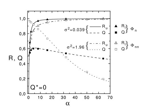
FIG. 1.: Order parameters of SVMs for purely linear teacher rules, $Q^{*}=0$. Symbols are experimental results for input space dimension $N=50$, corresponding to the two kinds of quadratic mappings, $\Phi_{n}$ with $a=1/\sqrt{N}$ (full symbols) and $\Phi_{nn}$ with normalizing factor $a=1$ (open symbols) respectively. Error bars are smaller than the symbols. The lines are solutions of equations (10-14), for $\Delta=(N+1)/2$ and $\sigma^{2}=Na^{2}/\Delta$ with $N=50$, and $a$ corresponding to each mapping.

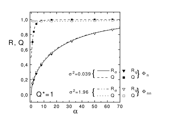
FIG. 2.: Order parameters of SVMs for purely quadratic teacher rules, $Q^{*}=1$. Definitions are the same as in figure 1.

FIG. 3.: Order parameters of SVMs for isotropic teacher rules, $Q^{*}_{iso}=\Delta/(1+\Delta)$. Definitions are the same as in figure 1.

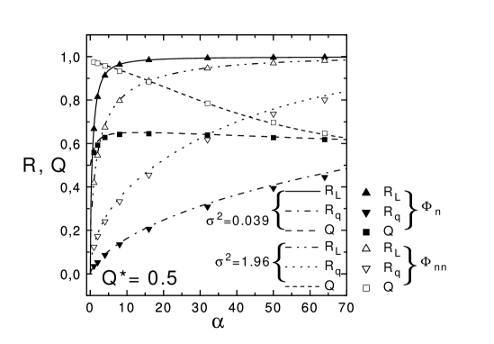
FIG. 4.: Order parameters of SVMs for a general teacher rule, $Q^{*}=0.5$. Definitions are the same as in figure 1.

We describe first the experimental data, obtained with quadratic SVMs, using both mappings, ${\mathchoice{{\hbox{\boldmath$\displaystyle\Phi$}}}{{\hbox{\boldmath$\textstyle\Phi$}}}{{\hbox{\boldmath$\scriptstyle\Phi$}}}{{\hbox{\boldmath$\scriptscriptstyle\Phi$}}}}_{nn}$ and ${\mathchoice{{\hbox{\boldmath$\displaystyle\Phi$}}}{{\hbox{\boldmath$\textstyle\Phi$}}}{{\hbox{\boldmath$\scriptstyle\Phi$}}}{{\hbox{\boldmath$\scriptscriptstyle\Phi$}}}}_{n}$, which have normalizing factors $a=1$ and $a=1/\sqrt{N}$ respectively, where $N$ is the input space dimension. The $M=\alpha N$ random input examples of each training set were selected with probability (1) and labelled by teachers of normalized weights ${\mathchoice{{\hbox{\boldmath$\displaystyle w$}}}{{\hbox{\boldmath$\textstyle w$}}}{{\hbox{\boldmath$\scriptstyle w$}}}{{\hbox{\boldmath$\scriptscriptstyle w$}}}}^{*}\equiv({\mathchoice{{\hbox{\boldmath$\displaystyle w$}}}{{\hbox{\boldmath$\textstyle w$}}}{{\hbox{\boldmath$\scriptstyle w$}}}{{\hbox{\boldmath$\scriptscriptstyle w$}}}}^{*}_{l},{\mathchoice{{\hbox{\boldmath$\displaystyle w$}}}{{\hbox{\boldmath$\textstyle w$}}}{{\hbox{\boldmath$\scriptstyle w$}}}{{\hbox{\boldmath$\scriptscriptstyle w$}}}}^{*}_{q})$ drawn at random. ${\mathchoice{{\hbox{\boldmath$\displaystyle w$}}}{{\hbox{\boldmath$\textstyle w$}}}{{\hbox{\boldmath$\scriptstyle w$}}}{{\hbox{\boldmath$\scriptscriptstyle w$}}}}^{*}_{l}$ are the $N$ components in the linear subspace and ${\mathchoice{{\hbox{\boldmath$\displaystyle w$}}}{{\hbox{\boldmath$\textstyle w$}}}{{\hbox{\boldmath$\scriptstyle w$}}}{{\hbox{\boldmath$\scriptscriptstyle w$}}}}^{*}_{q}$ are the $N^{2}$ components in the quadratic subspace. Notice that, because of the symmetry of the mappings, teachers having the same value of the symmetrized weights in the quadratic subspace, $(w^{*}_{q,ij}+w^{*}_{q,ji})/2$, are all equivalent. The teachers are characterized by the proportion of (squared) weight components in the quadratic subspace, $Q^{*}={\mathchoice{{\hbox{\boldmath$\displaystyle w$}}}{{\hbox{\boldmath$\textstyle w$}}}{{\hbox{\boldmath$\scriptstyle w$}}}{{\hbox{\boldmath$\scriptscriptstyle w$}}}}^{*}_{q}\cdot{\mathchoice{{\hbox{\boldmath$\displaystyle w$}}}{{\hbox{\boldmath$\textstyle w$}}}{{\hbox{\boldmath$\scriptstyle w$}}}{{\hbox{\boldmath$\scriptscriptstyle w$}}}}^{*}_{q}/{\mathchoice{{\hbox{\boldmath$\displaystyle w$}}}{{\hbox{\boldmath$\textstyle w$}}}{{\hbox{\boldmath$\scriptstyle w$}}}{{\hbox{\boldmath$\scriptscriptstyle w$}}}}^{*}\cdot{\mathchoice{{\hbox{\boldmath$\displaystyle w$}}}{{\hbox{\boldmath$\textstyle w$}}}{{\hbox{\boldmath$\scriptstyle w$}}}{{\hbox{\boldmath$\scriptscriptstyle w$}}}}^{*}$. In particular, $Q^{*}=0$ and $Q^{*}=1$ correspond to a purely linear and a purely quadratic teacher respectively.

The experimental student weights ${\mathchoice{{\hbox{\boldmath$\displaystyle w$}}}{{\hbox{\boldmath$\textstyle w$}}}{{\hbox{\boldmath$\scriptstyle w$}}}{{\hbox{\boldmath$\scriptscriptstyle w$}}}}\equiv({\mathchoice{{\hbox{\boldmath$\displaystyle w$}}}{{\hbox{\boldmath$\textstyle w$}}}{{\hbox{\boldmath$\scriptstyle w$}}}{{\hbox{\boldmath$\scriptscriptstyle w$}}}}_{l},{\mathchoice{{\hbox{\boldmath$\displaystyle w$}}}{{\hbox{\boldmath$\textstyle w$}}}{{\hbox{\boldmath$\scriptstyle w$}}}{{\hbox{\boldmath$\scriptscriptstyle w$}}}}_{q})$ were obtained by solving numerically the dual problem [5, 14], using the Quadratic Optimizer for Pattern Recognition program [15], that we adapted to the case without threshold treated in this paper. We determined $Q$, and the overlaps $R_{l}$ and $R_{q}$ in the linear and the quadratic subspaces, respectively. For each value of $M$, averages were performed over a large enough number of different teachers and training sets to get the precision shown in the figures.

Experiments were carried out for $N=50$. The corresponding feature space dimension is $N(N+1)=2550$. The restricted feature space considered in our model is composed of the $N$ (linear) input components, which define the u-subspace of the feature space, and the $N\Delta$ non redundant quadratic components of the $\sigma$-subspace. For the sake of comparison with the theoretical results determined in the thermodynamic limit, we caracterize the actual SVM by its (finite size) inflation factor $\Delta=(N+1)/2$, and the variance $\sigma^{2}$ of the components in the $\sigma$-subspace, related to the normalizing factor $a$ of the new features through $\sigma^{2}=Na^{2}/\Delta$. In our case, since $N=50$, $\Delta=25.5$ and $\sigma^{2}=1.960784a^{2}$, that is $\sigma^{2}=1.960784$ for the non-normalized mapping and $\sigma^{2}=0.039216$, for the normalized one.

The values of $Q$, the fraction of squared student weights in the $\sigma$-subspace, and the teacher-student overlaps $R_{u}$ and $R_{\sigma}$, normalized within the corresponding sub-space, are represented on figures 1 to 4 as a function of $\alpha\equiv M/N$, using full and open symbols for the mappings ${\mathchoice{{\hbox{\boldmath$\displaystyle\Phi$}}}{{\hbox{\boldmath$\textstyle\Phi$}}}{{\hbox{\boldmath$\scriptstyle\Phi$}}}{{\hbox{\boldmath$\scriptscriptstyle\Phi$}}}}_{n}$ and ${\mathchoice{{\hbox{\boldmath$\displaystyle\Phi$}}}{{\hbox{\boldmath$\textstyle\Phi$}}}{{\hbox{\boldmath$\scriptstyle\Phi$}}}{{\hbox{\boldmath$\scriptscriptstyle\Phi$}}}}_{nn}$ respectively. Notice that the abscissas correspond to the fraction of training patterns per input space dimension. Error bars are smaller than the symbols’ size. The lines are not fits, but the theoretical curves corresponding to the same classes of teachers as the experimental results. The excellent agreement with the experimental data is striking. Thus, the high order correlations of the features, neglected in the theoretical models, are indeed negligible.

Fig. 1 corresponds to a purely linear teacher ($Q^{*}=0$), i.e. to a quadratic SVM learning a rule linearly separable in input space. As in this case $R_{\sigma}=0$, only $R_{u}$ and $Q$ are represented. In the case of a purely quadratic rule, $Q^{*}=1$, represented on fig. 2, $R_{u}=0$. Notice that the corresponding overlaps, $R_{u}$ and $R_{\sigma}$, do not have a similar behaviour, as the latter increases much slower than the former, irrespective of the mapping. This happens because, as the number of quadratic components scales like $N\Delta$, a number of examples of the order of $N\Delta$ are needed to learn them. Indeed, $R_{u}$ reaches a value close to $1$ with $\alpha\sim O(1)$ while $R_{\sigma}$ needs $\alpha\sim O(\Delta)$ to reach similar values.

Fig. 3 shows the results corresponding to the isotropic teacher, having $Q^{*}=Q^{*}_{iso}\equiv\Delta/(1+\Delta)$. For $\Delta=25.5$ we have $Q^{*}_{iso}=0.962$ A particular case of such a teacher has all its weight components of equal absolute value, i.e. $(w_{i}^{*})^{2}=1/{\tilde{N}}$, and was studied in [8] and [6]. Finally, the results corresponding to a general rule, with $Q^{*}=0.5$, are shown in fig. 4. Notice that at fixed $\alpha$, $R_{u}$ decreases and $R_{\sigma}$ increases with $Q^{*}$ at a rate that depends on the mapping. These quantities determine the student’s generalization error through the combination (19). The fact that they increase as a function of $\alpha$ with different speed is a signature of hierarchical learning.

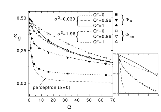
FIG. 5.: Learning curves of SVMs for different teacher rules $Q^{*}$. Definitions are the same as in figure 1. The inset is an enlargement of the smalll $\alpha$ region.

The generalization error $\epsilon_{g}$ corresponding to the different rules is plotted against $\alpha$ on fig. 5, for both mappings. At any fixed $\alpha$, the performance obtained with the normalized mapping is better the smaller the value of $Q^{*}$. The non-normalized mapping shows the opposite trend: its performance for a purely linear teacher is extremely bad, but it improves for increasing values of $Q^{*}$ and slightly overrides that of the normalized mapping in the case of a purely quadratic teacher. These results reflect the competition on learning the anisotropically distributed features. In the case of the normalized mapping, the $\sigma$-components are compressed ($\sigma^{2}=0.039$) with respect to the u-components, which have unit variance. This is advantageous whenever the linear components carry the most significant information, which is the case for $Q^{*}\ll 1$. When $Q^{*}=1$, the linear components only introduce noise that hinders the learning process. As the number of linear components is much smaller than the number of quadratic ones, their pernicious effect should be more conspicuous the smaller the value of $\Delta$. Conversely, the non-normalized mapping has $\sigma^{2}=1.96$, meaning that the compressed components are those of the u-subspace. Therefore, this mapping is better when most of the information is contained in the $\sigma$-subspace, which is the case for teachers with large $Q^{*}$ and, in particular, with $Q^{*}=1$.

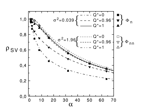
FIG. 6.: Fraction of learning patterns that belong to the subset of Support Vectors.

Finally, for the sake of completeness, the fraction of support vectors $\rho_{SV}\equiv M_{SV}/M$, where $M_{SV}$ is the number of training patterns with maximal stability, is represented on figure 6. This fraction is an upper bound to the generalization error. Notice that these curves present qualitatively the same trends as $\epsilon_{g}$. Interestingly, $\rho_{SV}$ is smaller for the normalized mapping than for the non-normalized one for most of the rules. Since the student’s weights can be expressed as a linear combination of SVs [1], this result is of practical interest.

IV Discussion

In order to understand the results obtained in the previous section, we first analyze the relative behaviour of $R_{u}$ and $R_{\sigma}$, which can be deduced from equation (13). If $\Delta^{*}_{\sigma}\ll\Delta$, which is the case for sufficiently small $Q^{*}$, we get that $R_{\sigma}\ll R_{u}$. This means that the quadratic components are more difficult to learn than the linear ones. On the other hand, if the teacher lies mainly in the quadratic subspace, $\Delta^{*}_{\sigma}\gg\Delta$, and then $R_{\sigma}>R_{u}$. The crossover between these different behaviours occurs at $\Delta^{*}_{\sigma}=\Delta$, for which equation (13) gives $R_{\sigma}=R_{u}$. For $N=50$, which is the case in our simulations, this arises for $Q^{*}_{n}=0.998$ or $Q^{*}_{nn}=0.929$, depending on whether we use the normalized or the non-normalized mapping. In the particular case of the isotropic teacher and the non-normalized mapping, $Q^{*}>Q^{*}_{nn}$, so that $R_{\sigma}>R_{u}$, as shown on figure 3. These considerations alone are not sufficient to understand the behaviour of the generalization error, which depends on the weighted sum of $R_{\sigma}$ and $R_{u}$ (see equation (19)).

The behaviour at small $\alpha$ is useful to understand the onset of hierarchical learning. A close inspection of equations (10-13) shows that in the limit $\alpha\rightarrow 0$, $x=\sigma^{2}$ and $Q\simeq\Delta\sigma^{2}/(\Delta\sigma^{2}+1)$ to leading order in $\alpha$. This results may be understood with the following simple argument: if there is only one training pattern, clearly it is a SV and the student’s weight vector is proportional to it. As a typical example has $N$ components of unit length in the u-subspace and $N\Delta$ components of length $\sigma$ in the $\sigma$-subspace, we have $Q=N\Delta\sigma^{2}/(N\Delta\sigma^{2}+N)$. With the normalized mapping, $\lim_{\alpha\rightarrow 0}Q=1/2$. In the case of the non normalized one $\lim_{\alpha\rightarrow 0}Q=(2\Delta-1)/2\Delta$, which depends on the inflation factor of the SVM. In this limit, we obtain:

$$\kappa_{max} \simeq \frac{1+\sigma^{2}\Delta}{\sqrt{1+\sigma^{4}\Delta}}\frac{1}{\sqrt{\alpha}},$$ (21)

$$R_{u} \simeq \sqrt{\frac{2}{\pi}}\frac{1}{\sqrt{1+\Delta^{*}_{\sigma}}}\sqrt{\alpha},$$ (22)

$$R_{\sigma} \simeq \sqrt{\frac{2}{\pi}}\,\sqrt{\frac{\Delta^{*}_{\sigma}}{1+\Delta^{*}_{\sigma}}}\,\sqrt{\frac{\alpha}{\Delta}}.$$ (23)

Therefore, $R\sim\sqrt{\alpha}$, like for the simple perceptron MMH [12], but with a prefactor that depends on the mapping and the teacher.

In our model, we expect that hierarchical learning correspond to a fast increase of $R$ at small $\alpha$, mainly dominated by the contribution of $R_{u}$. As in the limit $\alpha\rightarrow 0$,

$$R\simeq\frac{R_{u}+R_{\sigma}\sqrt{\sigma^{4}\Delta\Delta^{*}_{\sigma}}}{\sqrt{1+\sigma^{4}\Delta}\sqrt{1+\Delta^{*}_{\sigma}}},$$ (24)

we expect hierarchical learning if $\sigma^{4}\Delta\ll 1$ and $\Delta^{*}_{\sigma}\lesssim 1$. The first condition establishes a constraint on the mapping, which is only satisfied by the normalized one. The second condition, that ensures that $R_{\sigma}<R_{u}$ holds, gives the range of teachers for which this hierarchical generalization takes place. Under these conditions, $R$ grows fast and the contribution of $R_{\sigma}$ is negligible because it is weighted by $\sqrt{\sigma^{4}\Delta\Delta^{*}_{\sigma}}$. The effect of hierarchical learning is more important the smaller $\Delta^{*}_{\sigma}$. The most dramatic effect arises for $Q^{*}=0$, i.e. for a quadratic SVM learning a linearly separable rule.

On the other hand, if $\sigma^{4}\Delta\gg 1$, which is the case for the non normalized mapping, both $R_{u}$ and $R_{\sigma}$ contribute to $R$ with comparable weights. Notice that, if the normalized mapping is used, the condition $\Delta^{*}_{\sigma}\lesssim 1$ implies that $Q^{*}<Q^{*}_{iso}\equiv\Delta/(1+\Delta)$, where $Q^{*}_{iso}$ corresponds to the isotropic teacher. A straightforward calculation shows that a fraction of $47.5\%$ of teachers satisfies this constraint for $N=50$. In fact, the distribution of teachers as a function of $Q^{*}$ has its maximum at $Q^{*}_{iso}$. When $N\rightarrow\infty$, the distribution becomes $\delta(Q^{*}-Q^{*}_{iso})$, and $Q^{*}_{iso}$ tends to the median, meaning that in this limit, only about $50\%$ of the teachers give raise to hierarchical learning when using the normalized mapping.

In the limit $\alpha\rightarrow\infty$, all the generalization error curves converge to the same asymptotic value as the simple perceptron MMH learning in the feature space, namely $\epsilon_{g}=0.500489(1+\Delta)/\alpha$, independently of $\sigma$ and $Q^{*}$. Thus, $\epsilon_{g}$ vanishes slower the larger the inflation factor $\Delta$.

Finally, it is worth to point out that for $\sigma=1$, which would correspond to a normalizing factor $a=\sqrt{\Delta/N}$, the pattern distribution in feature space is isotropic. Irrespective of $Q^{*}$, the corresponding generalization error is exactly the same as that of a simple perceptron learning the MMH with isotropically distributed examples in feature space.

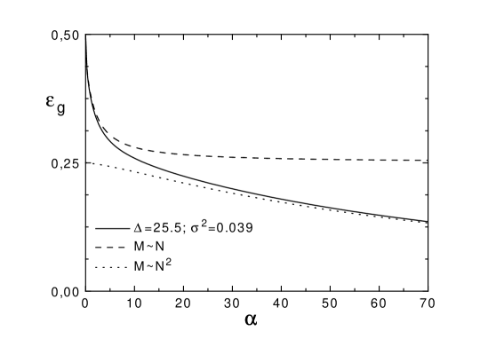
FIG. 7.: Generalization error of a SVM corresponding to different thermodynamic limits. See the text for the definition of $\alpha$ in each regime.

Since the inflation factor $\Delta$ of the SVM feature space in our approach is a free parameter, it does not diverge in the thermodynamic limit $N\rightarrow\infty$ . As a consequence, $\epsilon_{g}$ does not present any stepwise behaviour, but just a crossover between a fast decrease at small $\alpha$ followed by a slower decrease regime at large $\alpha$. The results of Dietrich et al. [6] for the normalized mapping, that corresponds to $\sigma^{2}\Delta=1$ in our model, can be deduced by taking appropriately the limits before solving our saddle point equations. The regime where the number of training patterns $M=\alpha N$ scales with $N$, is straightforward. It is obtained by taking the limit $\sigma\rightarrow 0$ and $\Delta\rightarrow\infty$ keeping $\sigma^{2}\Delta=1$ in our equations, with $\alpha$ finite. The regime where the number of training patterns $M=\alpha N$ scales with $N\Delta$, the number of quadratic features, obtained by keeping $\tilde{\alpha}\equiv\alpha/(1+\Delta)$ finite whilst taking, here again, the limit $\sigma\rightarrow 0$, $\Delta\rightarrow\infty$ with $\sigma^{2}\Delta=1$. The corresponding curves are represented on figure 7 for the case of an isotropic teacher. In order to make the comparisons with our results at finite $\Delta$, the regime where $\tilde{\alpha}$ is finite is represented as a function of $\alpha=(1+\Delta)\tilde{\alpha}$ using the value of $\Delta$ corresponding to our numerical simulations, namely, $\Delta=25.5$. In the same figure we represented the generalization error $\epsilon_{g}=(1/\pi)\arccos(R)$ where $R$, given by eq. (19), is obtained after solving the saddle point equations with parameter values $\sigma^{2}=0.039$ and $\Delta=25.5$.

These results, obtained for quadratic SVMs, are easily generalizable to higher order polynomial SVMs. The corresponding saddle point equations are cumbersome, and will not be given here. We expect a cascade of hierarchical generalization behaviour, in which successively more and more compressed features are learned. This may be understood by considering the set of saddle point equations that generalize equation (13). These equations relate the teacher-student overlaps in the successive subspaces. The sequence of different feature subspaces generalized by the SVM depends on the relative complexity of the teacher and the student. This is contained in the factors $\Delta^{*}_{\sigma_{m}}/\Delta_{m}$ corresponding to the $m^{th}$ subspace, that appear in the set of equations that generalize eq. (13).

V Conclusion

We introduced a model that clarifies some aspects of the generalization properties of polynomial Support Vector Machines (SVMs) in high dimensional feature spaces. To this end, we focused on quadratic SVMs. The quadratic features, which are the pairwise products of input components, may be scaled by a normalizing factor. Depending on its value, the generalization error presents very different behaviours in the thermodynamic limit [6, 7].

In fact, a finite size SVM may be caracterized by two parameters: $\Delta$ and $\sigma$. The inflation factor $\Delta$ is the ratio between the quadratic and the linear features dimensions. Thus, it is proportional to the input space dimension $N$. The variance $\sigma$ of the quadratic features is related to the corresponding normalizing factor. Usually, either $\sigma\sim 1/\sqrt{N}$ (normalized mapping) or $\sigma\sim 1$ (non normalized mapping). In previous studies, not only the input space dimension diverges in the thermodynamic limit $N\rightarrow\infty$, but also $\Delta$ and $\sigma$ are correspondingly scaled.

In our model, neither the proportion of quadratic features $\Delta$ nor their variance $\sigma$ are necessarily related to the input space dimension $N$. They are considered as parameters caracterizing the SVMs. Since we keep them constant when taking the thermodynamic limit, we can study the learning properties of actual SVMs with finite inflation ratios and normalizing factors, as a function of $\alpha\equiv M/N$, where $M$ is the number of training examples. Our theoretical results were obtained neglecting the correlations among the quadratic features. The agreement between our computer experiments with actual SVMs and the theoretical predictions is excellent. The effect of the correlations does not seem to be important, as there is almost no difference between the theoretical curves and the numerical results.

We find that the generalization error $\epsilon_{g}$ depends on the type of rule to be inferred through $Q^{*}$, the (normalized) sum of the teacher’s squared weight components in the quadratic subspace. If $Q^{*}$ is small enough, the quadratic components need more patterns to be learned than the linear ones. However, only if the quadratic features are normalized, $\epsilon_{g}$ is dominated by the high rate learning of the linear components at small $\alpha$. Then, on increasing $\alpha$, there is a crossover to a regime where the decrease of $\epsilon_{g}$ becomes much slower. The crossover between these two behaviours is smoother for larger values of $Q^{*}$, and this effect of hierarchical learning disappears for large enough $Q^{*}$. On the other hand, if the features are not normalized, the contributions of both the linear and the quadratic components to $\epsilon_{g}$ are of the same order, and there is no hierarchical learning at all.

In the case of the normalized mapping, if the limits $\Delta\sim N\rightarrow\infty$ and $\sigma^{2}\sim 1/N\rightarrow 0$ are taken together with the thermodynamic limit, the hierarchical learning effect gives raise to the two different regimes, corresponding to $M\sim N$ or $M\sim N^{2}$, described previously [8, 6].

It is worth to point out that if the rule to be learned allows for hierarchical learning, the generalization error of the normalized mapping is much smaller than that of the non normalized one. In fact, the teachers corresponding to such rules are those with $Q^{*}\lesssim Q^{*}_{iso}$, where $Q^{*}_{iso}$ corresponds to the isotropic teacher, the one having all its weights components equal. For the others, both the normalized mapping and the non normalized one present similar performances. If the weights of the teacher are selected at random on a hypersphere in feature space, the most probable teachers have precisely $Q^{*}=Q^{*}_{iso}$, and the fraction of teachers with $Q^{*}\leq Q^{*}_{iso}$ represent of the order of $50\%$ of the inferable rules. Thus, from a practical point of view, without having any prior knowledge about the rule underlying a set of examples, the normalized mapping should be preferred.

REFERENCES

- [1] V. Vapnik (1995) The nature of statistical learning theory. Springer Verlag, New York.
- [2] M. Opper, W. Kinzel, J. Kleinz and R. Nehl (1990) J. Phys. A: Math. Gen. 23, L-581.
- [3] M. Opper and W. Kinzel (1995) in Models of Neural Networks III, E. Domany, J.L. van Hemmen, K. Schulten (Eds.), pp. 151-209.
- [4] T. Cover (1965) IEEE Trans. Electron. Comput. 14, 326-334.
- [5] C. Cortes and V. Vapnik (1995) Machine Learning 20, 273-297.
- [6] R. Dietrich, M. Opper, and H. Sompolinsky (1999) Phys. Rev. Lett. 82, 2975-2978.
- [7] A. Buhot and M. B. Gordon (1999) ESANN’99-European Symposium on Artificial Neural Networks. Proceedings, Michel Verleysen ed., pp. 201-206; A. Buhot and M. B. Gordon (1998) cond-mat/9802179.
- [8] H. Yoon and J.-H. Oh (1998) J. Phys. A: Math. Gen. 31, 7771-7784.
- [9] R. Monasson (1993) J. Phys. A 25, 3701.
- [10] C. Marangi, M. Biehl and S. Solla (1995) Europhys. Lett. 30, 117-122.
- [11] S. Risau-Gusman and M. B. Gordon (2000) in Advances in Neural Information Processing Systems 12, edited by S. A. Solla, T. K. Leen, K-R. Muller (MIT Press), to be published.
- [12] M. B. Gordon and D. R. Grempel (1995) Europhys. Lett. 29, 257-262.
- [13] M. Opper (1988), Phys. Rev. A 38, 3824-3826.
- [14] R. J. Vanderbei (1998) Technical Report SOR-94-15, Princeton University.
- [15] Program available upon request to http://svm.first.gmd.de.