[

Toward a systematic $1/d$ expansion: Two particle properties

Abstract

We present a procedure to calculate $1/d$ corrections to the two-particle properties around the infinite dimensional dynamical mean field limit. Our method is based on a modified version of the scheme of Ref. [1]. To test our method we study the Hubbard model at half filling within the fluctuation exchange approximation (FLEX), a selfconsistent generalization of iterative perturbation theory. Apart from the inherent unstabilities of FLEX, our method is stable and results in causal solutions. We find that $1/d$ corrections to the local approximation are relatively small in the Hubbard model.

]

During the past few years dynamical mean field theory (DMFT) became one of the most popular methods to study strongly correlated systems [2]. DMFT developed from the path-breaking observation [3] that in the limit $d\to\infty$ of a $d$-dimensional lattice model with suitably rescaled hopping parameters, spatial fluctuations are completely suppressed and the self-energy becomes local. As a consequence, the self-energy can be written as a functional of the on-site Green’s function of the electrons and the lattice problem reduces to a quantum impurity problem, where the impurity is embedded in a selfconsistently determined environment. The main virtue of this method is that it captures all local time-dependent correlations and makes possible to study, e.g. the Mott-Hubbard transition or the phase diagram of different Kondo lattices in detail.

While in the case of the Mott-Hubbard transition the transition seems to be driven by the above-mentioned local fluctuations, in many cases correlated hopping [4] or inter-site interaction effects [5, 6] may play a crucial role as well, and while some of these effects can be qualitatively captured by a natural extension of the DMFT, others are beyond the scope of it and would only appear as $1/d$ corrections. Furthermore, in order to check the quality of the local approximation for a finite dimensional system of interest, it is very important to compare it with the size of the appearing $1/d$ corrections as well.

Several attempts have been made to partially restore some of the spatial correlations lost in the DMFT. One of the most successful ones is the cluster approximation proposed by Jarrell et al [7]. This method has the advantage of being causal, however, it requires considerable numerical prowess and it is not systematic in the small parameter $1/d$. Another method based on the systematic expansion of the generating functional has been suggested by Schiller and Ingersent [1]. However, despite of its technical and conceptual simplicity, this method has not been used very extensively because it seemed to be somewhat unstable and in some cases gave artificial non-causal solutions.

In the present work we first show, that the method of Schiller and Ingersent (SI) can be considerably stabilized by a minor, however crucial change in the algorithm, assuring that the contributions of some unwanted spurious diagrams exactly cancel. The price for this stability is a somewhat increased computation time, since in each cycle of the original algorithm an additional subcycle is needed to assure cancellation. With this change the SI method can then be safely extended to the calculation of two-particle properties. Here the main difficulties are connected to the inversion involved in the solution of the Bethe-Salpeter equation and the non-locality of the irreducible vertex functions. These difficulties are cicrcumvented by introducing bond variables for the two-particle propagators. Finally, we test the general formalism with the fluctuation exchange approximation (FLEX) [8].

Although the method presented applies to arbitrary lattice structures and various models with nearest neighbor interactions, for concreteness, let us consider the Hubbard model on a $d$-dimensional hypercubic lattice at half filling:

$$H={t\over\sqrt{d}}\sum_{<i,j>,\sigma}c^{\dagger}_{i\sigma}c_{j\sigma}+U\sum_{i}(n_{i\uparrow}-{1\over 2})(n_{i\downarrow}-{1\over 2})\;.$$ (1)

Here the dynamics of the conduction electrons $c_{i\sigma}$ is driven by the hopping $t$ between nearest neighbor sites, $n_{i\sigma}=c^{\dagger}_{i\sigma}c_{i\sigma}$ is the occupation number, and the electrons interact via the on-site Coulomb repulsion $U$.

In the SI formalism one considers the following single ($n=1$) and a two-impurity $(n=2)$ imaginary time effective functionals to generate $1/d$ corrections:

$$S^{(n)} = \sum_{\sigma}\sum_{\alpha,\beta=1}^{n}\int d\tau\int d\tau^{\prime}{\bar{c}}_{\alpha\sigma}(\tau)\bigl{[}{\cal G}^{(n)}\bigr{]}^{-1}_{\alpha,\beta}(\tau-\tau^{\prime})c_{\beta\sigma}(\tau^{\prime})$$ (2)

$$+ \sum_{\alpha=1}^{n}U\int d\tau n_{\alpha\uparrow}(\tau)n_{\alpha\downarrow}(\tau)\;.$$ (3)

Here, as usually, ${\bar{c}}_{\alpha\sigma}(\tau)$ and ${c}_{\alpha\sigma}(\tau)$ denote Grassman fields, and the indices $\alpha$ and $\beta$ label the sites for $n=2$ while they are redundant for $n=1$. The ’medium propagators’ ${\cal G}^{(1)}$ and ${\cal G}^{(2)}$ must be chosen in such a way that the dressed impurity propagators $G^{(1)}$ and $G^{(2)}$ coincide with the full on-site and nearest neighbor lattice propagators, $G^{\rm latt}_{00}$ and $G^{\rm latt}_{01}$:

$$G^{(1)}=G^{(2)}_{11}=G^{\rm latt}_{00}\;\phantom{n},\phantom{nnn}G^{(2)}_{12}=G^{\rm latt}_{01}\;.$$ (4)

In this case one can easily show that — restricting oneself to skeleton diagrams of the order of ${\cal O}(1/d)$ — the impurity self energies $\Sigma^{(1)}$ and $\Sigma^{(2)}_{\alpha\beta}$ and the diagonal and off-diagonal lattice self energies, $\Sigma^{\rm latt}_{0}$ and $\Sigma^{\rm latt}_{1}$ are related by [1]

$$\Sigma^{\rm latt}_{0} = \Sigma^{(1)}+2d(\Sigma^{(2)}_{11}-\Sigma^{(1)})\;,$$ (5)

$$\Sigma^{\rm latt}_{1} = \Sigma^{(2)}_{12}\;.$$ (6)

Knowing the lattice self energy the lattice Green function can then be expressed as

$$G_{lm}^{\rm latt}(i\omega)={1\over 1+\sqrt{d}\;\Sigma^{\rm latt}_{1}}G^{0}_{lm}\left({i\omega-\Sigma^{\rm latt}_{0}(i\omega)\over 1+\sqrt{d}\;\Sigma^{\rm latt}_{1}(i\omega)}\right)\;,$$ (7)

where $G^{0}_{lm}(z)$ and $G_{lm}^{\rm latt}(z)$ denote the unperturbed and dressed lattice propagators between sites $l$ and $m$, respectively.

Based on the relations above SI suggested the following simple iterative procedure to obtain a solution that includes ${\cal O}(1/d)$ corrections:

$${\cal G}^{(1,2)}\Rightarrow{\Sigma}^{(1,2)}\Rightarrow\Sigma^{\rm latt},G^{\rm latt}\Rightarrow{\cal G}^{(1,2)}\;.$$

A careful analysis shows, however, that the second step in this scheme is extremely unstable. To understand this it is enough to notice that the second term of Eq. (5) is constructed in such a way that at the fixed point all completely local skeleton diagrams in the expansion of $\Sigma^{(2)}_{11}$ are canceled by the subtracted $\Sigma^{(1)}$ term. However, this cancellation only happens under the condition that the dressed Green’s functions $G^{(2)}_{11}$ and $G^{(1)}$ are exactly the same. If $G^{(2)}_{11}$ and $G^{(1)}$ differ by a term of ${\cal O}(1/d)$ in a given iteration step, the cancellation above is not exact, and an error of the order of $2d\times{\cal O}(1/d)\sim 1$ is generated immediately. Moreover, the generated erroneous term is typically acausal because of the subtraction procedure involved in Eq. (5), and may drive the iteration towards some more stable but unphysical fixed point of the integral equations. We suggest to replace the critical steps ${\cal G}^{(1,2)}\Rightarrow{\Sigma}^{(1,2)}\Rightarrow\Sigma^{\rm latt}$ by the following procedure: (1) Calculate $G^{(2)}$ from ${\cal G}^{(2)}$, (2) Determine ${\cal G}^{(1)}$ selfonsistently in such a way that ${G}^{(1)}\equiv{G}^{(2)}_{11}$ be satisfied, (3) Determine $\Sigma^{(1,2)}$ and from them $\Sigma^{\rm latt}$. Step (2) above is crucial to guarantee that unwanted terms in Eq. (5) exactly cancel.

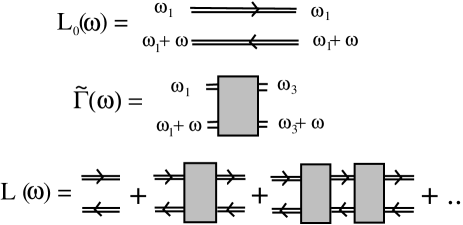
FIG. 1.: Graphical representation of the Bethe-Salpeter equation: Double lines indicate dressed Fermion propagators, while boxes denote particle-hole irreducible vertex diagrams.

The two-particle properties can be investigated in a way similar to Ref. [1]. To this end we introduce the lattice particle-hole irreducible vertex function ${\bf\tilde{\Gamma}}^{\rm latt}$, which is connected to the full lattice propagator ${\bf L}^{\rm latt}$ by the Bethe-Salpeter equation (see Fig. 1):

$${\bf L}^{\rm latt}(\omega)={\bf L}_{0}^{\rm latt}(\omega)({\bf 1}+{\bf\tilde{\Gamma}}^{\rm latt}(\omega){\bf L}_{0}^{\rm latt}(\omega))^{-1},$$ (8)

where $\omega$ denotes the transverse frequency and a tensor notation has been introduced in the spatial, spin and other frequency indices: $L(\omega)^{\sigma_{1},\sigma_{2};\sigma_{3},\sigma_{4}}_{i_{1},i_{2},\omega_{1};i_{3},i_{4},\omega_{3}}\to{\bf L}(\omega)$. The ’vertex-free’ propagator ${\bf L}_{0}^{\rm latt}(\omega)$ is defined as $L_{0}^{\rm latt}(\omega)^{\sigma_{1},\sigma_{2};\sigma_{3},\sigma_{4}}_{i_{1},i_{2},\omega_{1};i_{3},i_{4},\omega_{3}}=$ $\delta_{\sigma_{1}\sigma_{3}}\delta_{\sigma_{2}\sigma_{4}}\delta_{\omega_{1}\omega_{3}}$ $G_{i_{1},i_{3}}^{\rm latt}(i\omega_{1})$ $G_{i_{4},i_{2}}^{\rm latt}(i(\omega_{1}+\omega))$.

A detailed analysis shows that up to $1/d$ order the only non-zero matrix elements of ${\bf\tilde{\Gamma}}^{\rm latt}(\omega)$ are those where the indices $i_{1},i_{2},i_{3},i_{4}$ belong to the same or two nearest neighbor lattice sites, i.e. a bond. A thorough investigation of the corresponding skeleton diagrams shows that ${\bf\tilde{\Gamma}}^{\rm latt}(\omega)$ can be expressed similarly to Eqs. (5) and (6) as:

$${\bf\tilde{\Gamma}}^{\rm latt}=\left\{\mbox{ \begin{tabular}[]{ll }${\bf\tilde{\Gamma}}^{(1)}+2d({\bf\tilde{\Gamma}}^{(2)}-{\bf\tilde{\Gamma}}^{(1)})$&\phantom{n} $i_{1}=i_{2}=i_{3}=i_{4}$,\\ ${\bf\tilde{\Gamma}}^{(2)}$&\phantom{n} $i_{k}\in$ bond,\\ 0&\phantom{n}otherwise,\end{tabular} }\right.$$ (9)

where in the second line it is implicitely assumed that the $i_{k}$’s are not all equal. Here the particle-hole irreducible one- and two-impurity vertex functions, ${\bf\tilde{\Gamma}}^{(1)}$, and ${\bf\tilde{\Gamma}}^{(2)}$ are defined similarly to ${\bf\tilde{\Gamma}}^{\rm latt}$, and satisfy the impurity Bethe-Salpeter equation:

$${\bf L}^{(n)}(\omega)={\bf L}_{0}^{(n)}(\omega)({\bf 1}+{\bf\tilde{\Gamma}}^{(n)}(\omega){\bf L}_{0}^{(n)}(\omega))^{-1},$$ (10)

with $n=1,2$. Of course, in the impurity case the spatial indices of the propagators ${\bf L}_{0}^{(n)}(\omega)$ and ${\bf L}^{(n)}(\omega)$ are restricted to the impurity sites, but apart from this the ${\bf L}_{0}^{(n)}(\omega)$’s are equal to the lattice propagator ${\bf L}_{0}^{\rm latt}(\omega)$.

From the considerations above it immediately follows that the $1/d$ corrections to the two-particle properties can be calculated in the following way: (1) Find the solution of the single particle iteration scheme, (2) Determine the one- and two-impurity correlators, (3) Invert Eq. (10) to obtain ${\bf\tilde{\Gamma}}^{(1)}$ and ${\bf\tilde{\Gamma}}^{(2)}$, (4) Calculate ${\bf\tilde{\Gamma}}^{\rm latt}$ using Eq. (9), and (5) Solve the Bethe-Salpeter equation (8) for ${\bf L}^{\rm latt}$ and calculate two-particle response functions from it.

The major difficulties in the procedure above are associated with the inversion appearing in Eqs. (8), since the propagator ${\bf L}_{0}^{\rm latt}$ connects any four lattice sites and has an infinite number of frequency indices. The first difficulty can be resolved by observing that ${\bf\tilde{\Gamma}}^{\rm latt}$ connects only neighboring sites. Therefore with a introduction of bond variables a partial Fourier transformation can be carried out in these, and summations over all pairs of lattice sites reduce to a summation over $d$ ’bond direction indices’ and two additional indices specifying the position of the electron and the hole within a given bond. Furthermore, to avoid overcounting, the vertex function ${\bf\tilde{\Gamma}}^{\rm latt}$ must be replaced by a slightly modified ’bond vertex function’ [9]. A further reduction of the matrices involved can be achieved by diagonalizing the propagators in the spin labels. Finally, to carry out the summations and inversions over the infinite omega variables we introduced a frequency cutoff $\omega_{c}$ and extrapolated the $\omega_{c}=\infty$ result from a finite size scaling analysis in this cutoff [10], thereby reducing the numerical error of our calculations below one percent.

FIG. 2.: The generating functional for FLEX: Double lines denote single- and two-impurity dressed cavity propagators $G^{(1)}(\tau,\tau^{\prime})$ and $G^{(2)}(\tau,\tau^{\prime})$. Position and spin indices are not shown. The corresponding self-energy diagrams are obtained as $\Sigma(\tau-\tau^{\prime})=-\delta\phi[G(\tau,\tau^{\prime})]/\delta G(\tau^{\prime},\tau)$, and the particle-hole irreducible vertex is given by a similar second order functional derivative.

To test the procedure above one is tempted to try to generalize the iterative perturbation theory (IPT) applied remarkably successfully for the $d=\infty$ case [11], however, it is clear from the discussion above that within IPT it is impossible to satisfy the condition ${G}^{(1)}\equiv{G}^{(2)}_{11}$ (which explains why earlier attempts to generalize IPT to order $1/d$ failed [12]). We therefore applied the so-called fluctuation exchange approximation (FLEX) [8]. While this method is unable to capture the metal insulator transition, it is able to reproduce the Kondo resonance in the metallic phase[13], has been successfully used to calculate weak and intermediate coupling properties of the 2-dimensional Hubbard model [13], and it has the important property of being formulated in terms of the dressed single particle Green’s functions. In this approach the interactions between particles are mediated by fluctuations in the particle-particle and particle-hole channels, and the self-energies and the particle-hole (particle-particle) irreducible vertex functions are generated from the generating $\Phi$ functionals built in terms of the dressed Green’s functions, depicted in Fig. 2. A further advantage of FLEX is that due to the special structure of the diagrams involved a fast Fourier transform algorithm can be exploited to increase the speed and precision of the calculation substantially.

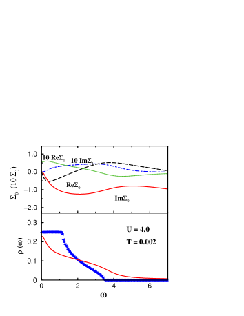
FIG. 3.: Top: Calculated diagonal and off-diagonal lattice self-energies for $U=4$ and $T=0.002$. All energies are measured in units of $t$. Bottom: Local spectral functions for $U=0$ and $U=4$ at $T=0.002$.

The calculated three-dimensional diagonal and off-diagonal lattice self-energies are shown in Fig. 3 together with the local spectral function. These have been obtained by means of a Pade approximation to carry out the analytic continuation from the imaginary to the real axis. Though in the spectral function a well-developed Kondo peak is observed, the FLEX is unable to reproduce the depletion of spectral weight in the neighborhood of it due to the ’over-regularization’ characteristic to most selfconsistent perturbative schemes. Remarkably, we experienced no convergence problems similar to those of Ref. [1], apart from the ones inherent in FLEX [8]. We checked that the spectral functions integrate to one within numerical precision and the solutions obtained are causal. The typical values of $\Sigma^{\rm latt}_{1}$ are nearly an order of magnitude smaller [14] than $\Sigma^{\rm latt}_{0}$, indicating that the local approximation gives surprisingly good results and $1/d$ corrections are indeed small as anticipated in Ref. [2] and also in agreement with the results of Ref. [1]. To get some further information about the quality of local approximation in Fig. 4 we plotted the momentum dependent spectral functions at different points of the Brillouin zone. The $1/d$ contributions give typically a 10-20 percent correction, but none of the generic properties is modified in the paramagnetic phase.

FIG. 4.: Momentum dependent spectral functions along the line $k=\alpha(\pi,\pi,\pi)$ within the local (dashed lines) and $1/d$ calculations (continuous lines). The alpha values used were $\alpha=0.497$, $\alpha=0.495$, and $\alpha=0.49$ from left to right. The energy of the quasiparticles has been renormalized approximately by a factor of four compared to the bare electron energies.

Once convergence is reached at the single particle level, one can turn to the two-particle properties. Within FLEX this is somewhat simpler, because — although many rather complicated diagrams are generated [8, 9] — ${\bf\tilde{\Gamma}}^{(n)}$ can be built up directly in terms of the full lattice Green’s functions. We find that similarly to the off-diagonal self-energy the off-diagonal elements of ${\bf\tilde{\Gamma}}^{\rm latt}$ are rather small. Having solved Eq. (8) one can calculate various correlation functions. As an example, in Fig. 5 we show the momentum dependent susceptibility of the half-filled Hubbard model in its paramagnetic phase for two different temperatures along the $(1,1,1)$ direction, obtained from the FLEX calculations. The susceptibility develops a peak at $(\pi,\pi,\pi)$ at low temperatures, as a sign of unstability toward antiferromagnetic phase transition.

We also determined the transition temperature at several values of $U$ and compared our results with existing Monte Carlo data[15]. We found a critical temperature $T_{c}$ typically by a factor of three lower than that of Ref. [15]. This difference is a result of the overregularization of the interaction vertex by FLEX. Indeed, replacing ${\bf\tilde{\Gamma}}^{\rm latt}(\omega)$ by the bare particle-hole vertex in Eq. (8) the order-parameter fluctuations become larger (see Fig. 5) and $T_{c}$ is in excellent agreement with the Monte Carlo data.

In conclusion, we presented an extended version of the SI method to calculate $1/d$ corrections to the two-particle properties. We tested the new procedure by FLEX. No convergence problems and no violation of causality appeared in our method, although this is not generally guaranteed within the present scheme. Our method should be tested on other models and with other, more time-consuming methods in the future as well.

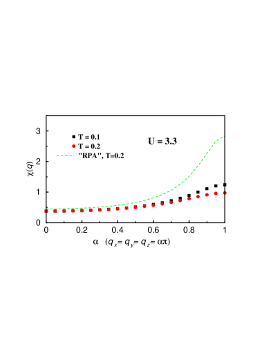
FIG. 5.: Momentum dependent susceptibilities. The susceptibility develops a peak at $(\pi,\pi,\pi)$ as a precursor of the antiferromagnetic phase transition.

The authors are grateful to N. Bickers for valuable discussions. This research has been supported by the U.S - Hungarian Joint Fund No. 587, grant No. DE-FG03-97ER45640 of the U.S DOE Office of Science, Division of Materials Research, and Hungarian Grant Nr. OTKA T026327, OTKA F29236, and OTKA T029813.

REFERENCES

- [1] A. Schiller and K. Ingersent, Phys. Rev. Lett. 75, 113 (1995).
- [2] For reviews see A. Georges, G. Kotliar, W. Krauth, and M. Rozenberg, Rev. Mod. Phys. 68, 13 (1996).
- [3] W. Metzner and D. Vollhardt, Phys. Rev. Lett. 62, 324 (1989).
- [4] A. Schiller (unpublished).
- [5] A. Pastor and V. Dobrosavljevic, Cond-Mat 9903272.
- [6] E. Müller-Hartmann, Z. Phys. B 74, 507 (1989); P.G.J. van Dongen, Phys. Rev. B 50, 14016 (1994).
- [7] M. Hettler et al., Rapid Comm. PRB 58, 7475 (1998); and Cond-Mat 9902267.
- [8] N. E. Bickers and D.J. Scalapino, Annals of Phys. 193, 206 (1989).
- [9] G. Zaránd, D.L. Cox, and A. Schiller (under preparation).
- [10] T. Pruschke, private communications, 1999.
- [11] A. Georges and G. Kotliar, Phys. Rev. B 45, 6479.
- [12] A. Georges (unpublished).
- [13] N.E. Bickers and C-X Chen, Solid State Comm. 82, 311 (1992). N.E. Bickers, D.J. Scalapino and S.R. White, Phys. Rev. Lett. 62, 961 (1989); C.-H. Pao and N. E. Bickers Phys. Rev. Lett 72, 1870 (1994).
- [14] In reality, appears with a prefactor in the Green’s function which, however, does not change this conclusion.
- [15] R. Scalettar, et al., Phys. Rev. B39, 4711 (1989).