Disorder Induced Transitions in Layered Coulomb Gases and Superconductors

Abstract

A 3D layered system of charges with logarithmic interaction parallel to the layers and random dipoles is studied via a novel variational method and an energy rationale which reproduce the known phase diagram for a single layer. Increasing interlayer coupling leads to successive transitions in which charge rods correlated in $N>1$ neighboring layers are nucleated by weaker disorder. For layered superconductors in the limit of only magnetic interlayer coupling, the method predicts and locates a disorder-induced defect-unbinding transition in the flux lattice. While $N=1$ charges dominate there, $N>1$ disorder induced defect rods are predicted for multi-layer superconductors.

Topological phase transitions induced by quenched disorder are relevant for numerous physical systems. Such transitions are likely to shape the phase diagram of type II superconductors. It was proposed [1] that the flux lattice (FL) remains a topologically ordered Bragg glass at low field, unstable to the proliferation of dislocations above a threshold disorder or field, providing one scenario for the controversial ”second peak” line [2, 3]. Another scenario [4] is based on a disorder-induced decoupling transition (DT) responsible for a sharp drop in the FL tilt modulus. Furthermore, for the pure system, it was shown recently [5] that in the absence of Josephson coupling, point ”pancake” vortices, i.e vacancies and interstitials in the FL, are nucleated at a temperature $T_{def}$, distinct from melting above some field. It is believed that this pure system topological transition merges with the thermal DT [6, 7] once the Josephson coupling is finite, being two anisotropic limits of the same transition [8] (at which superconducting order is destroyed while FL positional correlations are maintained). Thus an interesting possibility is that a similar, but now disorder-induced, vacancy-interstitial unbinding transition can be demonstrated in 3D layered superconductors, relevant to many layered and multilayer materials [2, 9].

In 2D recent progress was made to describe disorder induced topological transitions, in terms of Coulomb gases of charges with logarithmic long range interactions. It was shown [10, 11, 12, 13] that quenched random dipoles lead to a transition, via defect proliferation, at a finite threshold disorder, even at $T=0$.

In this Letter we develop a theory for a 3D defect-unbinding transition in presence of disorder. It is achieved for systems which can be mapped onto a layered Coulomb gas with quenched random dipoles, in which the interaction energy between two charges on layers $n$ and $n^{\prime}$ is $2J_{n-n^{\prime}}\ln r$ with $r$ the charge separation parallel to the layers. One physical realization is the FL in layered superconductors [2, 9, 14] with only magnetic coupling, for which we predict and locate the vacancy-interstitial unbinding transition. Indeed, as we argue, disorder induced deformations of the lattice result in random dipoles as seen by the defects. To study this problem we develop an efficient variational method which allows for fugacity distributions, known [13] to be important in 2D as they become broad at low $T$. We test the method on a single layer and reproduce the phase diagram, known from renormalization group (RG) with a $T=0$ disorder threshold $\sigma_{cr}=1/8$ [15]. For the 2-layer system we find that above a critical anisotropy $\eta\equiv-J_{1}/J_{0}=\eta_{c}=1-\frac{1}{\sqrt{2}}$ the single layer type transition is preempted by a transition induced by bound states of two pancake vortices on the two layers with $\sigma_{cr}<1/8.$ We develop a $T=0$ energy rationale by an approximate mapping to a Cayley tree problem and find that it reproduces the 2-layer result. Extension to many layers with only nearest layer coupling shows a cascade of transitions in which the number of correlated charges on $N$ neighboring layers increases, while the critical disorder decreases with $\eta$, with $N\rightarrow\infty$, $\sigma_{cr}\rightarrow 0$ as $\eta\rightarrow 1/2$. Finally we consider arbitrary range $n_{0}$ for $J_{n}$ with the constraint $\sum_{n}J_{n}=0$, as appropriate for layered superconductors. For $N>n_{0}^{2}$ states with $\sigma_{cr}\sim n_{0}^{2}/N\rightarrow 0$ are possible but only at exponentially large length scales for $n_{0}\gg 1$. Thus for layered superconductors we expect that the N=1 state dominates and find its phase diagram. Varying the system parameters by forming multilayers reduces $n_{0}$ and allows for realization of the new $N>1$ phases.

We study the Hamiltonian:

$${\cal H}=-\frac{1}{2}\sum_{{\bf r}\neq{\bf r}^{\prime}}\sum_{n,n^{\prime}}2J_{n-n^{\prime}}s_{n}({\bf r})\ln({\bf r}-{\bf r}^{\prime})s_{n^{\prime}}({\bf r}^{\prime})$$ (1)

$$-\sum_{{\bf r},n}V_{n}({\bf r})s_{n}({\bf r})$$ (2)

where $s_{n}({\bf r})=\pm 1,0$ define the positions ${\bf r}$ of charges on the $n$-th layer, $V_{n}({\bf r})$ is a disorder potential with long range correlations $\overline{V_{n}({\bf q})V_{n^{\prime}}({-\bf q})}=4\pi\sigma J_{0}^{2}\Delta_{n-n^{\prime}}/q^{2}$ with $\Delta_{0}=1$ (the short distance cutoff being set to unity). For simplicity we start with uncorrelated disorder from layer to layer $\Delta_{n-n^{\prime}}=\delta_{nn^{\prime}}$ with

$$\overline{[V_{n}({\bf r})-V_{n}({\bf r}^{\prime})]^{2}}=4\sigma J_{0}^{2}\ln|{\bf r}-{\bf r}^{\prime}|$$ (3)

representing quenched dipoles on each layer. At $T=0$ the problem amounts to find minimal energy configurations of charges in a logarithmically correlated random potential. For a single layer it was studied either using [10, 16] a “random energy model” (REM) approximation [17], or more accurately using a representation in terms of directed polymers on a Cayley tree (DPCT) [12] shown to emerge [13] (as a continuum branching process) from the Coulomb gas RG of the single layer problem. Schematically, the tree has independent random potentials (Fig. 1) $v_{i}$ on each bond with variance $\overline{v_{i}^{2}}=2\sigma J_{0}^{2}$. After $l$ generations one has $\sim e^{2l}$ sites which are mapped onto a 2D layer, i.e. two points separated by $r\sim e^{l}$ have a common ancestor at the previous $l\approx\ln r$ generation. Each point ${\bf r}$ has a unique path on the tree (DP) with $v_{1},...,v_{l}$ potentials and is assigned a potential $V({\bf r})=v_{1}+...+v_{l}$. Since all bonds previous to the common ancestor are identical $\overline{[V({\bf r})-V({\bf r}^{\prime})]^{2}}=2\sum_{i=1}^{l}\overline{v_{i}^{2}}$ reproducing (3) on each layer. Exact solution of the DPCT [18] yields the energy gained from disorder $V_{min}=min_{\bf r}V({\bf r})\approx-\sqrt{8\sigma}J_{0}\ln L$ for a volume $L^{2}$, with only $O(1)$ fluctuations [13], i.e $-\sqrt{8\sigma}J_{0}$ per generation $l=\ln L$.

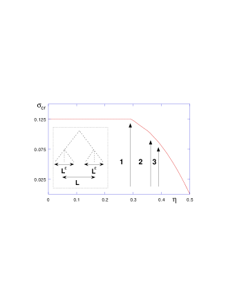
FIG. 1.: Critical disorder values with only nearest neighbor coupling $J_{1}$ vs. the anisotropy $\eta=-J_{1}/J_{0}$. Transitions between different $N$ phases are marked with arrows. Inset: the Cayley tree representation (for $N=3$ neighboring layers) with $+$ charges (at the tree endpoints) separated by $L^{\epsilon}$ along the layers, and separated by $L$ from the $N=3$ $-$ charges.

Optimal energy configurations for $M$ coupled layers are constructed considering $N$ neighboring layers with a $+,-$ pair on each layer and no charges on the other layers. We can take $J_{0}>0$ and $J_{n\neq 0}\leq 0$ so that equal charges on different layers attract. The DPCT representation now involves, on a single tree, $N$ $+$ polymers (each seeing different disorder) and $N$ $-$ polymers (each seeing opposite disorder $-v_{i}$ to their $+$ partner). A plausible configuration is that the $+$ charges bind within a scale $L^{\epsilon}$ ($0\leq\epsilon\leq 1$), so do the $-$ charges, while the $+$ to $-$ charge separations define the scale $L$. Its tree representation (Fig. 1) has $2N$ branches with $\epsilon\ln L$ generations, i.e. an optimal energy of $-2N\sqrt{8\sigma}J_{0}\epsilon\ln L$. On the scale between $L^{\epsilon}$ and $L$ the $+$ charges act as a single charge with a potential $\sum_{n=1}^{N}V_{n}({\bf r})$ (the $N$ polymers share the same branch) of variance $N\sigma$ hence the optimal energy is $-2\sqrt{8N\sigma}J_{0}(1-\epsilon)\ln L$. The total disorder energy is [19]:

$$E_{dis}\approx-2J_{0}\sqrt{8\sigma}[\epsilon N+(1-\epsilon)\sqrt{N}]\ln L\,.$$ (4)

The competing interaction energy $E_{int}$ is the sum of the one for the $+-$ pairs, $[2J_{0}N+4\sum_{n=1}^{N}J_{n}(N-n)]\ln L$ and for the $++/--$ pairs, $-4\sum_{n=1}^{N}J_{n}(N-n)\epsilon\ln L$. The total energy $E_{tot}=E_{dis}+E_{int}$ being linear in $\epsilon$, its minimum is at either $\epsilon=1$ or $\epsilon=0$. Since $\epsilon=1$ implies that the $+$ charges unbind, it is sufficient to consider $\epsilon=0$ with all $N\geq 1$, i.e. a rod with $N$ correlated charges has energy (with $\eta_{n}=-J_{n}/J_{0}$):

$$E_{tot}=2J_{0}N[1-2\sum_{n=1}^{N}\eta_{n}(1-\frac{n}{N})-\sqrt{\frac{8\sigma}{N}}]\ln L\,.$$ (5)

Disorder induces the $N$ vortex state at the critical value:

$$\sigma_{cr}=\frac{N}{8}[1-2\sum_{n=1}^{N}\eta_{n}(1-\frac{n}{N})]^{2}\,.$$ (6)

(i.e. $E_{tot}=0$). Consider first only nearest neighbor coupling $\eta_{l}=\eta_{1}\delta_{l1}$. Then $\sigma_{cr}$ is minimal at $N=1$ with $\sigma_{cr}=1/8$ if $\eta_{1}<1-1/\sqrt{2}$. For larger anisotropies successive $N$ states form at $1/(1-2\eta_{1})=1+\sqrt{N(N-1)}\sim N$ with diverging $N$ as $\eta_{1}\to\frac{1}{2}$ (Fig 1) [21].

Consider now $J_{n}$ of range $n_{0}$ constrained by $\sum_{n}J_{n}=0$ as for the superconductor, e.g. $\eta_{n}=\eta_{1}e^{-(n-1)/n_{0}}$ for which $\sigma_{cr}=(1-e^{-N/n_{0}})/8N(1-e^{-1/n_{0}})$. For $n_{0}\gg 1$, each $\eta_{n\neq 0}$ is small: for $N\lesssim n_{0}$ the lowest $\sigma_{cr}$ is at $N=1$. However, the combined strength of $N\approx n_{0}$ vortices being significant $\sigma_{cr}$ has a maximum and decreases back to zero for $N>n_{0}$ as $\sigma_{cr}\approx n_{0}^{2}/8N$. Hence $\sigma_{cr}\rightarrow 0$ as $N\rightarrow\infty$ and any small disorder seems to nucleate such vortices. This is because the perfect screening of the zero mode $\sum_{n}J_{n}=0$ implies that an infinite charge rod has a vanishing $\ln r$ interaction; hence a logarithmically correlated disorder is always dominant.

The realization of the large $N$ rods depends, however, on the type of thermodynamic limit. Adding to (5) the core energy $E_{c}N$ and minimizing yields a $N$-vortex scale

$$L\approx\exp\{E_{c}\sqrt{N}/[2J_{0}(\sqrt{8\sigma}-\sqrt{8\sigma_{cr}})]\}\,.$$ (7)

Hence as $\sigma\rightarrow 0$ such states are only achievable when $L/N$ diverges exponentially. Using $\sigma_{cr}\approx n_{0}^{2}/8N$, for $N>n_{0}^{2}/8\sigma$ the lowest scale $L$ in this range is achieved at $N=n_{0}^{2}/2\sigma$ and leads to a lower bound $L_{min}\approx\exp[E_{c}n_{0}/4J_{0}\sigma]$ for observing large $N$ states with a given $\sigma<\frac{1}{8}$. For layered superconductors $E_{c}/J_{0}\gg 1$ [22] and $n_{0}\gg 1$ and this large $N$ instability occurs at unattainable scales, thus $N=1$ dominates. One needs $n_{0}\approx 2-3$, as in multilayers, to realize the $N>1$ states.

To substantiate these results we develop a variational method for $M$ layers which allows for fugacity distributions, an essential feature in the one-layer problem. Disorder averaging (2) in Fourier using replicas yields:

$$\beta{\cal H}_{r}=\frac{1}{2d^{2}}\int_{k}\int_{q}s_{a}({\bf q},k)(G_{0})_{ab}({\bf q},k)s_{b}^{*}({\bf q},k)$$ (8)

$$+\beta E_{c}\sum_{{\bf r},n}s_{na}^{2}({\bf r})$$ (9)

where $(G_{0})_{ab}({\bf q},k)=(4\pi/q^{2})[g(k)\delta_{ab}-\sigma J_{0}^{2}\beta^{2}\Delta(k)]$, $g(k)=\beta J(k)=\beta d\sum_{n}J_{n}\exp(ikdn)$, $d$ the interlayer spacing [24] (for uncorrelated layers $\Delta(k)=d$), $a,b=1,...,m$ are replica indices and $m\rightarrow 0$ is to be carefully taken. In transforming to a sine-Gordon Hamiltonian [8] it is crucial to keep all charge fugacities [13], which yields:

$$\beta{\cal H}_{SG}=\frac{1}{2}\int_{kq}\chi_{a}({\bf q},k)(G_{0})^{-1}_{ab}\chi^{*}_{b}({\bf q},k)$$ (10)

$$-\sum_{{\bf r}}\sum_{{\bf s}\neq{\bf 0}}Y[{\bf s}]\exp(i{\bf s}\cdot{\mbox{\boldmath$\chi$}}({\bf r}))\quad.$$ (11)

¿From now on ${\bf s}=\{s_{na}\}_{n=1,.M,a=1,.m}$ is an integer vector both in layer label and replica space (i.e. of length m M) of entries $0,\pm 1$ and the summation is over all such non null vectors (also $\chi({\bf r})\equiv\{\chi_{n,a}({\bf r})\}$, ${\bf s}\cdot{\mbox{\boldmath$\chi$}}=\sum_{na}s_{na}\chi_{na}$). We now look for the best gaussian approximation of (11) with propagator $G^{-1}_{ab}({\bf q},k)=(G_{0})^{-1}_{ab}({\bf q},k)+\sigma_{c}(k)\delta_{ab}+\sigma_{0}(k)$. The bare fugacity being $Y[{\bf s}]=\exp{(-\beta E_{c}\sum_{n,a}s_{n,a}^{2})}$ the naive approach would be to restrict to charges ${\bf s}$ with a single non zero entry, leading to a uniform fugacity term $-y\sum_{{\bf r},n,a}\cos({\mbox{\boldmath$\chi$}_{na}}({\bf r}))$ and a diagonal $k$-independent replica mass term. Instead we keep all composite charges ${\bf s}$, which allow for variational solutions with off diagonal and $k$-dependent replica mass terms. This corresponds respectively to fluctuations of fugacity and $N>1$ charge rods being generated and becoming relevant as also seen from RG. The variational free energy is ${\cal F}_{var}={\cal F}_{0}+\langle{\cal H}_{SG}-{\cal H}_{0}\rangle_{0}$ where $\langle...\rangle$ is an average using $\beta{\cal H}_{0}=\frac{1}{2}\int_{{\bf q},k}\chi_{a}({\bf q},k)G_{ab}({\bf q},k)\chi^{*}_{b}({\bf q},k)$ and $\beta{\cal F}_{0}=-\frac{1}{2}\text{tr}\ln G$. The Gaussian average $F[{\bf s}]\equiv Y[{\bf s}]\langle\exp{i{\bf s}\cdot{\mbox{\boldmath$\chi$}}({\bf r})}\rangle_{0}$ yields:

$$F[{\bf s}]=\exp\{-\frac{1}{2d^{2}}\int_{k}\sum_{ab}(\tilde{G}_{c}(k)\delta_{ab}-A(k))s_{a}(k)s^{*}_{b}(k)\}$$ (12)

$$G_{c}(k)=g(k)\ln[\Lambda/(4\pi g(k)\sigma_{c}(k))]$$ (13)

$$A(k)=\sigma\beta^{2}J_{0}^{2}\Delta(k)(G_{c}(k)/g(k)-1)+g(k)\sigma_{0}(k)/\sigma_{c}(k)$$ (14)

where $s_{a}(k)=d\sum_{n}s_{na}e^{iknd}$, $\tilde{G}_{c}(k)=G_{c}(k)+2\beta E_{c}d$, $\Lambda$ the UV cutoff on $q^{2}$. $F_{var}$ is minimized by $\sigma_{c}(k)\delta_{ab}+\sigma_{0}(k)=\Lambda d^{-2}\sum_{{\bf s}}s_{a}(k)s_{b}^{*}(k)F[{\bf s}]$. Writing the $A(k)$ term as an average over $M$ random gaussian fugacities ${w_{k}}$:

$$\exp{\{\frac{1}{2}|\sum_{a}s_{a}(k)|^{2}A(k)\}}=\langle\exp{w_{k}\sum_{a}s_{a}(k)}\rangle_{w}$$ (15)

where $\langle...\rangle_{w}=\prod_{k}\int...e^{-|w_{k}|^{2}/2A(k)}d^{2}w_{k}/\sqrt{2\pi A(k)}$, allows to perform the exact sum on replicas yielding $\sum_{{\bf s}}F[{\bf s}]=\langle Z^{m}\rangle_{w}$ with $Z=\sum_{\{s_{n}=0,\pm 1\}}\exp(-\frac{1}{2d^{2}}\int_{k}\tilde{G}_{c}(k)|s(k)|^{2}+\frac{1}{d}\int_{k}w_{k}s^{*}(k))$. The variational equations for $m\rightarrow 0$ become [20]

$$\sigma_{c}(k)=\Lambda\langle\frac{\partial^{2}\ln Z}{\partial w_{k}\partial w^{*}_{k}}\rangle_{w}\,;{\mbox{\hskip 5.69054pt}}\sigma_{0}(k)=\Lambda\langle|\frac{\partial\ln Z}{\partial w_{k}}|^{2}\rangle_{w}$$ (16)

For a single layer $k=0$ and $Z=1+e^{u+w}+e^{u-w}$, $2u=-\tilde{G}_{c}(0)/d$, $w=w_{0}$ is a trinomial. (16) can be solved for the critical line where $\sigma_{c}(0)\rightarrow 0$. The phase diagram shown in Fig. 2 (full line) reproduces precisely recent RG results. The variational scheme, allowing for all replica charges ${\bf s}$, therefore treats disorder correctly. For two layers $kd=0,\pi$ we need two fugacity distributions $w_{0},w_{\pi}$ and $Z$ is a ”ninomial”, i.e. $Z=1+$ eight exponentials involving $G_{c}(0)$, $G_{c}(\pi)$. Focusing on the low $T$ boundary, where $\sigma_{c}(\pi)\sim[\sigma_{c}(0)]^{\alpha}\rightarrow 0$ we find [20] either (i) $\alpha=1$ for $\eta_{1}<\eta_{c}=1-1/\sqrt{2}$, representing decoupled layers, or (ii) $\alpha\rightarrow\infty$ for $\eta_{1}>\eta_{c}$, representing a $++$ bound states on the two layers. The $T=0$ energy rationale is therefore reproduced. The phase diagram for two layers with $\eta_{c}<\eta<1/2$ is shown in Fig. 2 [15]

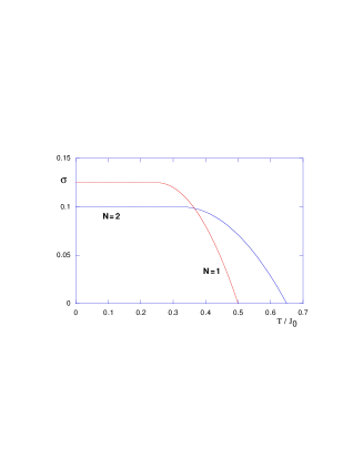
FIG. 2.: Phase diagram for the onset of the $N=1,2$ instabilities for anisotropy $\eta=0.35$. At low $T$ two distinct transitions are possible, the first being to the rod $N=2$ phase. At high $T$ the independent layer $N=1$ transition dominates

For any number of layers one obtains a simple $N$ rod solution by restricting the sum over ${\bf s}$ in (11) to a subclass of charges of the form $s_{na}=s_{a}\sum_{j=1,N}\delta_{n,n^{\prime}+j-1}$. The variational solution, of the form $\sigma_{c}(k)=\sigma_{c}\phi_{N}(k)$, reduces to an effective one layer problem, in term of the structure factor of the rod $s_{a}(k)s_{b}^{*}(k)=\phi_{N}(k)\equiv\sin^{2}(Nkd/2)/\sin^{2}(kd/2)$. The $N$ rod becomes critical at:

$$\sigma_{cr}=(\int_{k}\phi_{N}(k)J(k))^{2}/(8J_{0}^{2}\int_{k}\phi_{N}(k)\Delta(k))$$ (17)

a formula which can equivalently be obtained within the Cayley tree rationale. Indeed for any correlations $\Delta_{n}$, the energy of the $\epsilon=0$ configurations is still given by (5) replacing $\sigma\to\sigma(1+2\sum_{n=1}^{N}\Delta_{n}(1-n/N))$). (17) reproduces both single (using $\phi(0)=N$) and two layer results. Finally, for many layers and weak interlayer coupling (e.g. $\eta_{1}<1-1/\sqrt{2}$ in Fig.1) the $N=1$ transition dominates and occurs at $\sigma_{cr}=1/8$ ((17) using $\phi_{1}(k)=1$).

As a direct application we consider a flux lattice in a layered superconductor with no Josephson coupling and a magnetic field $B$ perpendicular to the layers. The FL is composed of pancake vortices displaced from the $p$-th line position ${\bf R}_{p}$ at the $n$-th layer into ${\bf R}_{p}+{\bf u}_{p}^{n}$. The defects $s_{n}({\bf r})$ couple to the lattice via ${\cal H}_{vac}=\sum_{{\bf r},p,n,n^{\prime}}s_{n^{\prime}}({\bf r})G_{v}({\bf R}_{p}+{\bf u}_{p}^{n}-{\bf r},n^{\prime}-n)$ where, in Fourier [8] $G_{v}({\bf q},k)=(\phi_{0}^{2}d^{2}/4\pi\lambda_{ab}^{2}q^{2})/[1+f({\bf q},k)]$ where $f({\bf q},k)=(d/4\lambda_{ab}^{2}q)\sinh qd/[\sinh^{2}(qd/2)+\sin^{2}(kd/2)]$; $\phi_{0}=Ba^{2}$ is the flux quantum, $a$ the FL spacing, $\lambda_{ab}$ the penetration length along the layers. To 0-th order in ${\bf u}_{p}^{n}$ the defects feel a periodic potential fixing their position in a unit cell, hence $s({\bf q},k)$ involve only $|q|<1/a$.

In the limit $q\to 0$ the longitudinal modes, to which defects couple, have for (tilt) elastic energy [23] ${\cal H}_{el}=\frac{1}{2d^{2}a^{4}}\int_{kq}D(k)|{\bf u}_{L}({\bf q},k)|^{2}$ with $D(k)=\frac{1}{2}\sum_{{\bf Q}\neq 0}[G_{v}({\bf Q},k)-G_{v}({\bf Q},0)]+G_{v}(k)$ where ${\bf Q}$ are reciprocal wavevectors of the lattice and $G_{v}(k)=\lim_{q\rightarrow 0}G_{v}({\bf q},k)q^{2}=\phi_{0}^{2}d^{2}k_{z}^{2}/[4\pi(1+\lambda_{ab}^{2}k_{z}^{2})]$ and $k_{z}=(2/d)\sin(kd/2)$. The sum on ${\bf Q}$ is due to the high momentum components of the magnetic field and is responsible for the non-perfect screening of the defect interaction and to a finite $T_{def}$. Minimizing ${\cal H}_{vac}+{\cal H}_{el}$ yields ${\bf u}_{vac}({\bf q},k)=i{\bf q}s({\bf q},k)G_{v}(k)a^{2}/D(k)q^{2}$ and (8) with:

$$g(k)=\beta G_{v}(k)[1-G_{v}(k)/D(k)]/4\pi$$ (18)

Thus the long range interaction is $\sim\ln r$ and its coefficient determines $T_{def}=2J_{0}$ (via $\int_{k}g(k)=2$). Since $\int_{k}G_{v}(k)\sim\phi_{0}^{2}d/\lambda_{ab}^{2}$, the scale of the melting transition [14], the defect transition occurs before melting and can thus be consistently described only if $D(k)-G_{v}(k)\ll D(k)$. This is possible if either $d\ll a\ll\lambda_{ab}$ where $g(k)=\beta d\tau^{\prime}\ln(1+a^{2}k_{z}^{2}/4\pi)$ with $\tau^{\prime}=\phi_{0}^{2}da^{2}/(128\pi^{3}\lambda_{ab}^{4})$ and [5] $T_{def}=\tau^{\prime}ln(a/d)$ or for $d>a$ where $g(k)=\beta(d^{4}/a)\tau^{\prime}k_{z}^{2}e^{-2\pi d/a}$ leading to $T_{def}=4(d/a)\tau^{\prime}e^{-2\pi d/a}$. Remarkably $D(k)-G_{v}(k)\ll D(k)$ also yields that the long range response ${\bf u}_{vac}({\bf r})\sim a^{2}{\bf r}/r^{2}$ to a vacancy at ${\bf r}=0$ is confined to the same layer.

Point disorder deforms the flux lattice, producing quenched dipoles coupling to our defects. Expansion of the disorder energy, valid below the Larkin length [1], and minimization together with ${\cal H}_{vac}+{\cal H}_{el}$ yields readily (2). A more general argument, valid at all scales, treats $u_{vac}$ as a small perturbation around the Bragg glass configuration. Systematic expansion of the free energy $F=F_{BG}+\frac{1}{d^{2}a^{2}}\int_{qk}iqs(q,k)G_{v}(q,k)\langle u(q,k)\rangle_{s=0}+O(s^{2})$ in defect density in a given disorder configuration shows that a defect feels a logarithmically correlated random potential $V_{l}({\bf r})$ as in (2, 8) with $\sigma J_{0}^{2}\Delta(k)=G_{v}(k)^{2}\lim_{q\to 0}C_{BG}(q,k)/4\pi d^{2}a^{4}$ where $C_{BG}({\bf r},l)=\overline{\langle u^{L}_{0}({\bf 0})\rangle\langle u^{L}_{l}({\bf r})\rangle}$ is the correlation in the unperturbed Bragg glass $C_{BG}(0,k)\sim 1/(c^{2}_{44}(k^{4}+R_{c}^{-1}k^{3})$, $R_{c}$ a Larkin length along $c$ [1]. It yields a $k$-independent $\Delta(k)$ for $k>1/R_{c}$ while $\Delta(k)\sim k$ for $k<1/R_{c}$.

Applications to FL depends on the interlayer form of (18) of range $n_{0}\approx a/d$ for large $a/d$. Remarkably $g(k=0)=0$, i.e perfect screening holds as in 2D [5]. Hence $\sum_{n}J_{n}=0$ and as $n_{0}$ is reduced $J_{0},J_{1}$ dominate the sum, i.e. $\eta_{1}\rightarrow\frac{1}{2}$ when $d\gg a$. One finds that $\eta_{1}$ crosses the critical value $1-1/\sqrt{2}$ when $d/a\approx 1$, depending weakly on $a/\lambda_{ab}$. We thus propose that FL in multilayer superconductors, where $d>a$ can be achieved, can show a rich phase diagram with $N>1$ phases. In layered superconductors $a/d\approx 10-100$ [2] and the $N=1$ transition at $\sigma_{cr}=1/8$ dominates for realistic sizes. The disorder-induced decoupling transition, neglecting defects, predicted [7] at $\sigma_{dec}=2$ is thus above the defect transition (with $B\sim\sigma$) in the $B-T$ plane (similarly thermal decoupling occurs at $T_{dec}=8T_{def}$ for $d\ll a\ll\lambda$). A natural scenario is again of a single transition at $\sigma_{c}$ varying from $2$ to $1/8$ as the bare Josephson coupling is reduced, e.g. by increasing $d$ in multilayers.

In conclusion, we developed a variational method and a Cayley tree rationale to study layered Coulomb gas. The results are relevant to flux lattices where we find the phase boundaries and propose new $N>1$ phases for $d\gtrsim a$. The present methods may be useful for other 2D disordered systems, such as quantum Hall.

This work was supported by the French-Israeli program Arc-en-ciel and by the Israel Science Foundation.

REFERENCES

• [1] T. Giamarchi, P. Le Doussal, Phys. Rev. B 52 1242 (1995) and Phys. Rev. B 55 6577 (1997).
• [2] P. H. Kes, J. Phys. I France 6 2327 (1996).
• [3] B. Kaykovich et al. Phys. Rev. Lett 76 2555 (1996), K. Deligiannis et al. Phys. Rev. Lett 79 2121 (1997).
• [4] B. Horovitz, cond-mat/9903167, Phys. Rev. B 60 R9939 (1999).
• [5] M. J. W. Dodgson, V. B. Geshkenbein and G. Blatter Phys. Rev. Lett. 83 5358 (1999).
• [6] L. Daemen et al., Phys. Rev. Lett. 70, 1167 (1993)
• [7] B. Horovitz and T. R. Goldin, Phys. Rev. Lett. 80,1734 (1998).
• [8] B. Horovitz, Phys. Rev. B47, 5947 (1993)
• [9] Y. Bruynseraede et al., Phys. Scr. T42, 37 (1992).
• [10] T. Nattermann et al., J. Phys. I (France) 5, 565 (1995)
• [11] S. Scheidl, Phys. Rev. B 55, 457 (1997)
• [12] L. H. Tang, Phys. Rev. B 54, 3350 (1996).
• [13] D. Carpentier and P. Le Doussal, Phys. Rev. Lett. 81 2558 (1998), cond-mat/9908335 and in preparation.
• [14] G. Blatter et al. Rev. Mod. Phys. 66 1125 (1994).
• [15] these phase diagrams are exact in terms of renormalized parameters $\sigma_{R}$, $g_{R}(k)$ as seen from RG studies[13, 20].
• [16] B. Derrida Phys. Rev. B 24 2613 (1981)
• [17] i.e. replacing the $V({\bf r})$ by $L^{2}$ variables uncorrelated in ${\bf r}$, with the same on-site variance $\overline{V^{2}({\bf r})}\sim 2\sigma J_{0}^{2}\ln L$ also yielding [16] $V_{min}\sim-\sqrt{8\sigma}J_{0}\ln L$.
• [18] B. Derrida, H. Spohn, J. Stat. Phys. 51 817 (1988).
• [19] an upper bound which can be argued to be exact [20].
• [20] B. Horovitz and P. Le Doussal in preparation.
• [21] if $\eta_{1}>\frac{1}{2}$ the defects form a lattice even without disorder.
• [22] $E_{c}/J_{0}\approx(\lambda_{ab}/a)^{2}/\ln(a/d)$ in that case.
• [23] T. R. Goldin and B. Horovitz, Phys. Rev. B58, 9524 (1998).
• [24] with $\int_{q}\equiv\int\frac{d^{2}q}{(2\pi)^{2}}$, $\int_{k}\equiv\frac{1}{Md}\sum_{k}\to\int_{-\pi/d}^{\pi/d}\frac{dk}{2\pi}$ for large $M$, $s_{a}({\bf q},k)=d\sum_{n,{\bf r}}s_{na}({\bf r})e^{i{\bf q}{\bf r}+ikdn}$ and $\beta=1/T$.