SU-4240-714 The Statistical Mechanics of Membranes

Abstract

The fluctuations of two-dimensional extended objects (membranes) is a rich and exciting field with many solid results and a wide range of open issues. We review the distinct universality classes of membranes, determined by the local order, and the associated phase diagrams. After a discussion of several physical examples of membranes we turn to the physics of crystalline (or polymerized) membranes in which the individual monomers are rigidly bound. We discuss the phase diagram with particular attention to the dependence on the degree of self-avoidance and anisotropy. In each case we review and discuss analytic, numerical and experimental predictions of critical exponents and other key observables. Particular emphasis is given to the results obtained from the renormalization group $\varepsilon$-expansion. The resulting renormalization group flows and fixed points are illustrated graphically. The full technical details necessary to perform actual calculations are presented in the Appendices. We then turn to a discussion of the role of topological defects whose liberation leads to the hexatic and fluid universality classes. We finish with conclusions and a discussion of promising open directions for the future.

1 Introduction

The statistical mechanics of one-dimensional structures (polymers) is fascinating and has proved to be fruitful from the fundamental and applied points of view [1, 2]. The key reasons for this success lie in the notion of universality and the relative simplicity of one-dimensional geometry. Many features of the long-wavelength behavior of polymers are independent of the detailed physical and chemical nature of the monomers that constitute the polymer building blocks and their bonding into macromolecules. These microscopic details simply wash out in the thermodynamic limit of large systems and allow predictions of critical exponents that should apply to a wide class of microscopically distinct polymeric systems. Polymers are also sufficiently simple that considerable analytic and numerical progress has been possible. Their statistical mechanics is essentially that of ensembles of various classes of random walks in some $d$-dimensional bulk or embedding space.

A natural extension of these systems is to intrinsic two-dimensional structures which we may call generically call membranes. The statistical mechanics of these random surfaces is far more complex than that of polymers because two-dimensional geometry is far richer than the very restricted geometry of lines. Even planar two-dimensional — monolayers — are complex, as evidenced by the KTNHY [3, 4, 5] theory of defect-mediated melting of monolayers with two distinct continuous phase transitions separating an intermediate hexatic phase, characterized by quasi-long-range bond orientational order, from both a low-temperature crystalline phase and a high-temperature fluid phase. But full-fledged membranes are subject also to shape fluctuations and their macroscopic behavior is determined by a subtle interplay between their particular microscopic order and the entropy of shape and elastic deformations. For membranes, unlike polymers, distinct types of microscopic order (crystalline, hexatic, fluid) will lead to distinct long-wavelength behavior and consequently a rich set of universality classes.

Flexible membranes are an important member of the enormous class of soft condensed matter systems [6, 7, 8, 9], those which respond easily to external forces. Their physical properties are to a considerable extent dominated by the entropy of thermal fluctuations.

In this review we will describe some of the presently understood behavior of crystalline (fixed-connectivity), hexatic and fluid membranes, including the relevance of self-avoidance, intrinsic anisotropy and topological defects. Emphasis will be given to the role of the renormalization group in elucidating the critical behavior of membranes. The polymer pastures may be lovely but a dazzling world awaits those who wander into the membrane meadows.

The outline of the review is the following. In sec. 2 we describe a variety of important physical examples of membranes, with representatives from the key universality classes. In sec. 3 we introduce basic notions from the renormalization group and some formalism that we will use in the rest of the review. In sec. 4 we review the phase structure of crystalline membranes for both phantom and self-avoiding membranes, including a thorough discussion of the fixed-point structure, RG flows and critical exponents of each global phase. In sec. 5 we turn to the same issues for intrinsically anisotropic membranes, with the new feature of the tubular phase. In sec. 6 we address the consequences of allowing for membrane defects, leading to a discussion of the hexatic membrane universality class. We end with a brief discussion of fluid membranes in sec. 7 and conclusions.

2 Physical examples of membranes

There are many concrete realizations of membranes in nature, which greatly enhances the significance of their study. Crystalline membranes, sometimes termed tethered or polymerized membranes, are the natural generalization of linear polymer chains to intrinsically two-dimensional structures. They possess in-plane elastic moduli as well as bending rigidity and are characterized by broken translational invariance in the plane and fixed connectivity resulting from relatively strong bonding. Geometrically speaking they have a preferred two-dimensional metric. Let’s look at some of the examples. One can polymerize suitable chiral oligomeric precursors to form molecular sheets [10]. This approach is based directly on the idea of creating an intrinsically two-dimensional polymer. Alternatively one can permanently cross-link fluid-like Langmuir-Blodgett films or amphiphilic bilayers by adding certain functional groups to the hydrocarbon tails and/or the polar heads [11, 12] as shown schematically in Fig. 1.

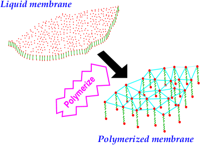
Figure 1: The polymerization of fluid-like membrane to a crystalline membrane.

The cytoskeletons of cell membranes are beautiful and naturally occurring crystalline membranes that are essential to cell membrane stability and functionality. The simplest and most thoroughly studied example is the cytoskeleton of mammalian erythrocytes (red blood cells). The human body has roughly $5\times 10^{13}$ red blood cells. The red blood cell cytoskeleton is a fishnet-like network of triangular plaquettes formed primarily by the proteins spectrin and actin. The links of the mesh are spectrin tetramers (of length approximately 200 nm) and the nodes are short actin filaments (of length 37 nm and typically 13 actin monomers long) [13, 14], as seen in Fig.3 and Fig.3. There are roughly 70,000 triangular plaquettes in the mesh altogether and the cytoskeleton as a whole is bound by ankyrin and other proteins to the cytoplasmic side of the fluid phospholipid bilayer which constitutes the other key component of the red blood cell membrane.

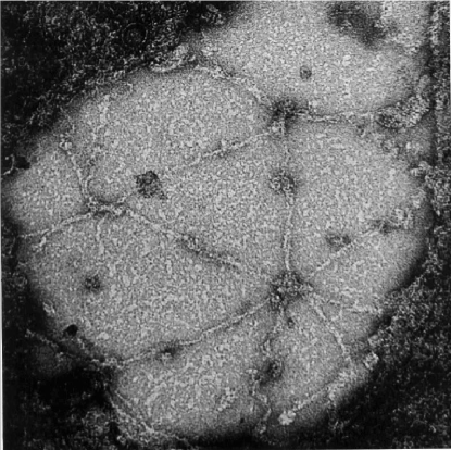
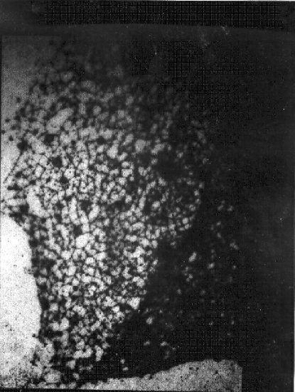
Figure 2: An electron micrograph of a region of the erythrocyte cytoskeleton. The skeleton is negatively stained (magnification 365,000) and has been artificially spread to a surface area nine to ten times as great as in the native membrane [15].

Figure 3: An extended view of the crystalline spectrin/actin network which forms the cytoskeleton of the red blood cell membrane [16].

There are also inorganic realizations of crystalline membranes. Graphitic oxide (GO) membranes are micron size sheets of solid carbon with thicknesses on the order of 10Å, formed by exfoliating carbon with a strong oxidizing agent. Their structure in an aqueous suspension has been examined by several groups [17, 18, 19]. Metal dichalcogenides such as MoS₂ have also been observed to form rag-like sheets [20]. Finally similar structures occur in the large sheet molecules, shown in Fig.4, believed to be an ingredient in glassy $B_{2}O_{3}$.

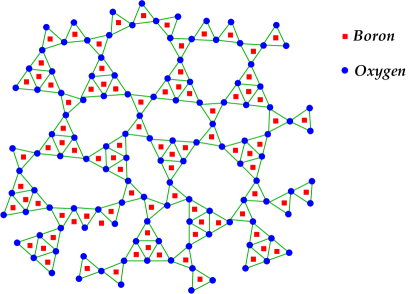
Figure 4: The sheet molecule $B_{2}O_{3}$

In contrast to crystalline membranes, fluid membranes are characterized by vanishing shear modulus and dynamical connectivity. They exhibit significant shape fluctuations controlled by an effective bending rigidity parameter.

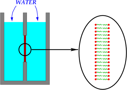
Figure 5: Schematic of experimental procedure to make a black membrane.

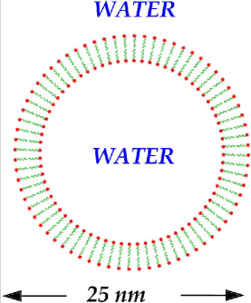
Figure 6: The structure of a liposome with its pure lipid spherical bilayer

A rich source of physical realizations of fluid membranes is found in amphiphilic systems [21, 22, 23]. Amphiphiles are molecules with a two-fold character – one part is hydrophobic and another part hydrophilic. The classic examples are lipid molecules, such as phospholipids, which have polar or ionic head groups (the hydrophilic component) and hydrocarbon tails (the hydrophobic component). Such systems are observed to self-assemble into a bewildering array of ordered structures, such as monolayers, planar (see Fig.5) and spherical bilayers (vesicles or liposomes) (see Fig. 6) as well as lamellar, hexagonal and bicontinuous phases [24]. In each case the basic ingredients are thin and highly flexible surfaces of amphiphiles. The lipid bilayer of cell membranes may itself be viewed as a fluid membrane with considerable disorder in the form of membrane proteins (both peripheral and integral) and with, generally, an attached crystalline cytoskeleton, such as the spectrin/actin mesh discussed above.

A complete understanding of these biological membranes will require a thorough understanding of each of its components (fluid and crystalline) followed by the challenging problem of the coupled system with thermal fluctuations, self-avoidance, potential anisotropy and disorder. The full system is currently beyond the scope of analytic and numerical methods but there has been considerable progress in the last fifteen years.

Related examples of fluid membranes arise when the surface tension between two normally immiscible substances, such as oil and water, is significantly lowered by the surface action of amphiphiles (surfactants), which preferentially orient with their polar heads in water and their hydrocarbon tails in oil. For some range of amphiphile concentration both phases can span the system, leading to a bicontinuous complex fluid known as a microemulsion. The oil-water interface of a microemulsion is a rather unruly fluid surface with strong thermal fluctuations [25] (see Fig.8).

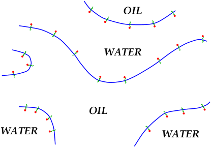
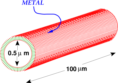
Figure 7: The structure of a microemulsion formed by the addition of surfactant to an oil-water mixture.

Figure 8: Metal-coated fluid microcylinders (tubules) formed by chiral lipids.

The structures formed by membrane/polymer complexes are of considerable current theoretical, experimental and medical interest. To be specific it has recently been found that mixtures of cationic liposomes (positively charged vesicles) and linear DNA chains spontaneously self-assemble into a coupled two-dimensional smectic phase of DNA chains embedded between lamellar lipid bilayers [26, 27]. For the appropriate regime of lipid concentration the same system can also form an inverted hexagonal phase with the DNA encapsulated by cylindrical columns of liposomes[28] (see Fig.9). In both these structures the liposomes may act as non-viral carriers (vectors) for DNA with many potentially important applications in gene therapy [29]. Liposomes themselves have long been studied and utilized in the pharmaceutical industry as drug carriers [30].

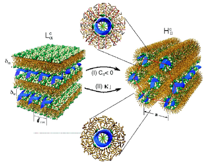
Figure 9: The lamellar and inverted hexagonal DNA-membrane complexes from the work of [28]

On the materials science side the self-assembling ability of membranes is being exploited to fabricate microstructures for advanced material development. One beautiful example is the use of chiral-lipid based fluid microcylinders (tubules) as a template for metallization. The resultant hollow metal needles may be half a micron in diameter and as much as a millimeter in length [31, 32], as illustrated in Fig.8. They have potential applications as, for example, cathodes for vacuum field emission and microvials for controlled release [31].

3 The Renormalization Group

The Renormalization Group (RG) has provided an extremely general framework that has unified whole areas of physics and chemistry [33]. It is beyond the scope of this review to discuss the RG formalism in detail but there is an ample literature to which we refer the reader (see the articles in this issue). It is the goal of this review to apply the RG framework to the statistical mechanics of membranes, and for this reason we briefly emphasize and review some well known aspects of the RG and its related $\varepsilon$-expansion.

The RG formalism elegantly shows that the large distance properties (or equivalently low $p$-limit) of different models are actually governed by the properties of the corresponding Fixed Point (FP). In this way one can compute observables in a variety of models, such as a molecular dynamics simulation or a continuum Landau phenomenological approach, and obtain the same long wavelength result. The main idea is to encode the effects of the short-distance degrees of freedom in redefined couplings. A practical way to implement such a program is the Renormalization Group Transformation (RGT), which provides an explicit prescription for integrating out all the high $p$-modes of the theory. One obtains the large-distance universal term of any model by applying a very large ($\infty$ to be rigorous) number of RGTs.

The previous approach is very general and simple but presents the technical problem of the proliferation in the number of operators generated along the RG flow. There are established techniques to control this expansion, one of the most successful ones being the $\varepsilon$-expansion. The $\varepsilon$-expansion may also performed via a field theoretical approach using Feynman diagrams and dimensional regularization within a minimal subtraction scheme, which we briefly discuss below. Whereas it is true that this technique is rather abstract and intuitively not very close to the physics of the model, we find it computationally much simpler.

Generally we describe a particular model by several fields $\{\phi,\chi,\cdots\}$ and we construct the Landau free energy by including all terms compatible with the symmetries and introducing new couplings $(u,v,\cdots)$ for each term. The Landau free energy may be considered in arbitrary dimension $d$, and then, one usually finds a Gaussian FP (quadratic in the fields) which is infrared stable above a critical dimension ($d_{U}$). Below $d_{U}$ there are one or several couplings that define relevant directions. One then computes all physical quantities as a function of $\varepsilon\equiv d_{U}-d$, that is, as perturbations of the Gaussian theory.

In the field theory approach, we introduce a renormalization constant for each field $(Z_{\phi},Z_{\chi},\cdots)$ and a renormalization constant $(Z_{u},Z_{v},\cdots)$ for each relevant direction below $d_{U}$. If the model has symmetries, there are some relations among observables (Ward identities) and some of these renormalization constants may be related. This not only reduces their number but also has the added bonus of providing cross-checks in practical calculations. Within dimensional regularization, the infinities of the Feynman diagrams appear as poles in $\varepsilon$, which encode the short-distance details of the model. If we use these new constants ($Z$’s) to absorb the poles in $\varepsilon$, thereby producing a complete set of finite Green’s functions, we have succeeded in carrying out the RG program of including the appropriate short-distance information in redefined couplings and fields. This particular prescription of absorbing only the poles in $\varepsilon$ in the $Z$’s is called the Minimal Subtraction Scheme (MS), and it considerably simplifies practical calculations.

As a concrete example, we consider the theory of a single scalar field $\phi$ with two independent coupling constants. The one-particle irreducible Green’s function has the form

$$\Gamma^{N}_{R}({\bf k}_{i};u_{R},v_{R},M)=Z^{N/2}_{\phi}\Gamma^{N}({\bf k}_{i};u,v;\frac{1}{\varepsilon})\ ,$$ (1)

where the function on the left depends on a new parameter $M$, which is unavoidably introduced in eliminating the poles in $\varepsilon$. The associated correlator also depends on redefined couplings $u_{R}$ and $v_{R}$. The rhs depends on the poles in $\varepsilon$, but its only dependence on $M$ arises through $Z_{\phi}$. This observation allows one to write

$$M\frac{d}{dM}\left(Z_{\phi}^{-N/2}\Gamma_{R}^{(N)}\right)=$$

$$= \left(M\frac{\partial}{\partial M}+\beta(u_{R})\frac{\partial}{\partial u_{R}}+\beta(v_{R})\frac{\partial}{\partial v_{R}}-\frac{N}{2}\Gamma_{\phi}\right)\Gamma_{R}^{(N)}=0\ ,$$

where

$$u_{R}=M^{-\varepsilon}F(Z_{\phi},Z_{\chi},\cdots|Z_{u})u \ , v_{R}=M^{-\varepsilon}F(Z_{\phi},Z_{\chi},\cdots|Z_{v})v$$ (3)

$$\beta_{u}(u_{R},v_{R})=\left.\left(M\frac{\partial u_{R}}{\partial M}\right)\right|_{u,v} \ , \beta_{v}(u_{R},v_{R})=\left.\left(M\frac{\partial v_{R}}{\partial M}\right)\right|_{u,v}$$

$$\gamma_{\phi} = \left.\left(M\frac{\partial\ln Z_{\phi}}{\partial M}\right)\right|_{u,v}\ .$$

The $\beta$-functions control the running of the coupling by

$$M\frac{du_{R}}{dM}=\beta_{u}(u_{R},v_{R})\ ,\ M\frac{dv_{R}}{dM}=\beta_{v}(u_{R},v_{R})$$ (4)

The existence of a FP, at which couplings cease to flow, requires $\beta(u_{R}^{\ast},v_{R}^{\ast})=0$ for all $\beta$-functions of the model. Those are the most important aspects of the RG we wanted to review. In Appendix B we derive more appropriate expressions of the RG-functions for practical convenience. For a detailed exposition of the $\varepsilon$-expansion within the field theory framework we refer to the excellent book by Amit[34].

4 Crystalline Membranes

A crystalline membrane is a two dimensional fish-net structure with bonds (links) that never break - the connectivity of the monomers (nodes) is fixed. It is useful to keep the discussion general and consider $D$-dimensional objects embedded in $d$-dimensional space. These are described by a $d$-dimensional vector ${\vec{r}}({\bf x})$, with ${\bf x}$ the $D$-dimensional internal coordinates, as illustrated in Fig.10. The case $(d=3,D=2)$ corresponds to the physical crystalline membrane.

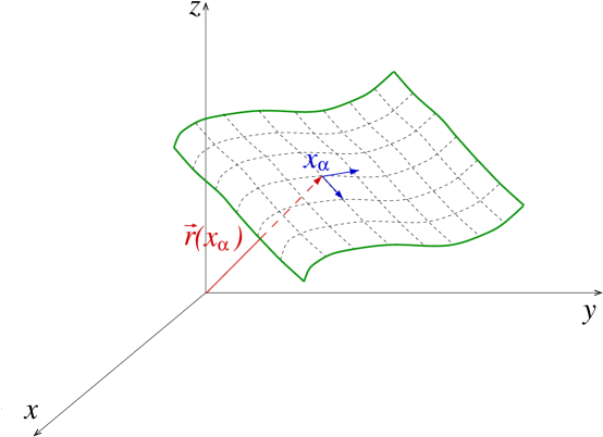
Figure 10: Representation of a membrane.

To construct the Landau free energy of the model, one must recall that the free energy must be invariant under global translations, so the order parameter is given by derivatives of the embedding ${\vec{r}}$, that is ${\vec{t}}_{\alpha}=\frac{\partial{\vec{r}}}{\partial u_{\alpha}}$, with $\alpha=1,\cdots,D$. This latter condition, together with the invariance under rotations (both in internal and bulk space), give a Landau free energy [35, 36, 37]

$$F({\vec{r}}) = \int d^{D}{\bf x}\left[\frac{1}{2}\kappa(\partial_{\alpha}^{2}{\vec{r}})^{2}+\frac{t}{2}(\partial_{\alpha}{\vec{r}})^{2}+u(\partial_{\alpha}{\vec{r}}\partial_{\beta}{\vec{r}})^{2}+v(\partial_{\alpha}{\vec{r}}\partial^{\alpha}{\vec{r}})^{2}\right]$$ (5)

$$+ \frac{b}{2}\int d^{D}{\bf x}\,d^{D}{\bf y}\delta^{d}({\vec{r}}({\bf x})-{\vec{r}}({\bf y}))\ ,$$

where higher order terms may be shown to be irrelevant at long wavelength, as discussed later. The physics in Eq.(5) depends on five parameters,

• $\kappa$, bending rigidity : This is the coupling to the extrinsic curvature (the square of the Gaussian mean curvature). Since reparametrization invariance is broken for crystalline membranes, this term may be replaced by its long-wavelength limit. For large and positive bending rigidities flatter surfaces are favored.

• $t,u,v$, elastic constants : These coefficients encode the microscopic elastic properties of the membrane. In a flat phase, they may be related to the Lamé coefficients of Landau elastic theory (see sect. 4.1.3).

• $b$, Excluded volume or self-avoiding coupling : This is the coupling that imposes an energy penalty for the membrane to self-intersect. The case $b=0$, i. e. no self-avoidance, corresponds to a phantom model.

We generally expand ${\vec{r}}({\bf x})$ as

$${\vec{r}}({\bf x})=(\zeta{\bf x}+{\bf u}({\bf x}),h({\bf x}))\ ,$$ (6)

with ${\bf u}$ the $D$-dimensional phonon in-plane modes, and $h$ the $d-D$ out-of-plane fluctuations. If $\zeta=0$ the model is in a rotationally invariant crumpled phase, where the typical surfaces have fractal dimension, and there is no real distinction between the in-plane phonons and out-of plane modes. For a pictorial view, see cases a) and b) in Fig.11.

If $\zeta\neq 0$ the membrane is flat up to small fluctuations and the full rotational symmetry is spontaneously broken. The fields $h$ are the analog of the Goldstone bosons and they have different naive scaling properties than ${\bf u}$. See Fig.11 for a visualization of a typical configuration in the flat phase.

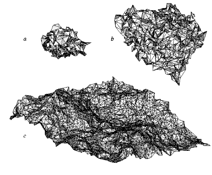
Figure 11: Examples of a) crumpled phase, b) crumpling transition (crumpled phase) and c) a flat phase. Results correspond to a numerical simulation of the phantom case [38] and gives a very intuitive physical picture of the different phases.

We will begin by studying the phantom case first. This simplified model may even be relevant to physical systems since one can envision membranes that self-intersect (at least over some time scale). One can also view the model as a fascinating toy model for understanding the more physical self-avoiding case to be discussed later. Combined analytical and numerical studies have yielded a thorough understanding of the phase diagram of phantom crystalline membranes.

4.1 Phantom

The Phantom case corresponds to setting $b=0$ in the free energy Eq.(5):

$$F({\vec{r}})=\int d^{D}{\bf x}\left[\frac{1}{2}\kappa(\partial_{\alpha}^{2}{\vec{r}})^{2}+\frac{t}{2}(\partial_{\alpha}{\vec{r}})^{2}+u(\partial_{\alpha}{\vec{r}}\partial_{\beta}{\vec{r}})^{2}+v(\partial_{\alpha}{\vec{r}}\partial^{\alpha}{\vec{r}})^{2}\right]\ .$$ (7)

The mean field effective potential, using the decomposition of Eq.(6), becomes

$$V(\zeta)=D\zeta^{2}(\frac{t}{2}+(u+vD)\zeta^{2})\ ,$$ (8)

with solutions

$$\zeta^{2}=\left\{\begin{array}[]{r@{\quad:\quad}l}0&t\geq 0\\ -\frac{t}{4(u+vD)}&t<0\ .\end{array}\right.$$ (9)

There is, consequently, a flat phase for $t<0$ and a crumpled phase for $t>0$, separated by a crumpling transition at $t=0$ (see Fig.12).

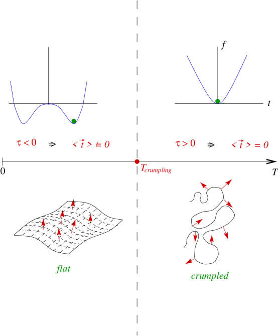
Figure 12: Mean field solution for crystalline membranes.

The actual phase diagram agrees qualitatively with the phase diagram of the model shown schematically in Fig.13. The crumpled phase is described by a line of equivalent FPs(GFP). There is a general hyper-surface, whose projection onto the $\kappa-t$ plane corresponds to a one-dimensional curve (CTH), which corresponds to the crumpling transition. Within the CTH there is an infrared stable FP (CTFP) which describes the large distance properties of the crumpling transition. Finally, for large enough values of $\kappa$ and negative values of $t$, the system is in a flat phase described by the corresponding infra-red stable FP (FLFP) . Although the precise phase diagram turns out to be slightly more complicated than the one depicted in Fig.13, the additional subtleties do not modify the general picture.

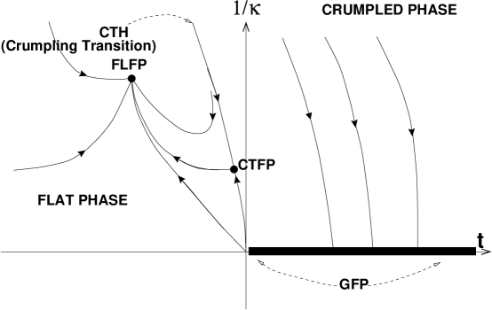
Figure 13: Schematic plot of the phase diagram for phantom membranes. GFP are the equivalent FPs describing the crumpled phase. The crumpling transition is described by the Crumpling transition critical line (CTH), which contains the Crumpling Transition FP (CTFP). The Flat phase is described by the (FLFP).

The evidence for the phase diagram depicted in Fig.13 comes from combining the results of a variety of analytical and numerical calculations. We present in detail the results obtained from the $\varepsilon$-expansion since they have wide applicability and allow a systematic calculation of the $\beta$-function and the critical exponents. We also describe briefly results obtained with other approaches.

4.1.1 The crumpled phase

In the crumpled phase, the free energy Eq.(7) for $D\geq 2$ simplifies to

$$F({\vec{r}})=\frac{t}{2}\int d^{D}{\bf x}(\partial_{\alpha}{\vec{r}})^{2}+\mbox{Irrelevant terms}\ ,$$ (10)

since the model is completely equivalent to a linear sigma model in $D\leq 2$ dimensions having $O(d)$ symmetry, and therefore all derivative operators in ${\vec{r}}$ are irrelevant by power counting. The parameter $t$ labels equivalent Gaussian FPs, as depicted in Fig.13. In RG language, it defines a completely marginal direction. This is true provided the condition $t>0$ is satisfied. The large distance properties of this phase are described by simple Gaussian FPs and therefore the connected Green’s function may be calculated exactly with result

$$G({\bf x})\sim\left\{\begin{array}[]{c l}|{\bf x}|^{2-D}&D\neq 2\\ \log|{\bf x}|&D=2\end{array}\right.$$ (11)

The associated critical exponents may also be computed exactly. The Hausdorff dimension $d_{H}$, or equivalently the size exponent $\nu=D/d_{H}$, is given (for the membrane case $D=2$) by

$$d_{H}=\infty\ (\nu=0)\rightarrow R_{G}^{2}\sim\log L\ .$$ (12)

The square of the radius of gyration $R_{G}^{2}$ scales logarithmically with the membrane size $L$. This result is in complete agreement with numerical simulations of tethered membranes in the crumpled phase where the logarithmic behavior of the radius of gyration is accurately checked [39, 40, 41, 42, 43, 44, 45, 46, 47, 38]. Reviews may be found in [48, 49].

4.1.2 The Crumpling Transition

The Free energy is now given by

$$F({\vec{r}})=\int d^{D}{\bf x}\left[\frac{1}{2}(\partial_{\alpha}^{2}{\vec{r}})^{2}+u(\partial_{\alpha}{\vec{r}}\partial_{\beta}{\vec{r}})^{2}+\hat{v}(\partial_{\alpha}{\vec{r}}\partial^{\alpha}{\vec{r}})^{2}\right]\ ,$$ (13)

where the dependence on $\kappa$ may be included in the couplings $u$ and $\hat{v}$. With the leading term having two derivatives, the directions defined by the couplings $u$ and $\hat{v}$ are relevant by naive power counting for $D\leq 4$. This shows that the model is amenable to an $\varepsilon$-expansion with $\varepsilon=4-D$. For practical purposes, it is more convenient to consider the coupling $v=\hat{v}+\frac{u}{D}$. We provide the detailed derivation of the corresponding $\beta$ functions in Appendix D. The result is

$$\begin{array}[]{c c r}\beta_{u}(u_{R},v_{R})&=&-\varepsilon u_{R}+\frac{1}{8\pi^{2}}\left\{(d/3+65/12)u^{2}_{R}+6u_{R}v_{R}+4/3v^{2}_{R}\right\}\\ \beta_{v}(u_{R},v_{R})&=&-\varepsilon v_{R}+\frac{1}{8\pi^{2}}\left\{21/16u^{2}_{R}+21/2u_{R}v_{R}+(4d+5)v^{2}_{R}\right\}\end{array}$$ (14)

Rather surprisingly, this set of $\beta$ functions does not possess a FP, except for $d>219$. This result would suggest that the crumpling transition is first order for $d=3$. Other estimates, however, give results which are consistent with the crumpling transition being continuous. These are

• Limit of large elastic constants[50]: The Crumpling transition is approached from the flat phase, in the limit of infinite elastic constants. The model is

  $$H_{NL}=\int d^{D}\sigma\frac{\kappa}{2}(\Delta{\vec{r}})^{2}\ ,$$ (15)

  with the further constraint ${\partial_{\alpha}\vec{r}}{\partial_{\beta}\vec{r}}=\delta_{\alpha\beta}$. Remarkably, the $\beta$-function may be computed within a large $d$ expansion, yielding a continuous crumpling transition with size exponent at the transition (for $D=2$)

  $$d_{H}=\frac{2d}{d-1}\rightarrow\nu=1-\frac{1}{d}\ .$$ (16)

• SCSA Approximation[51]: The Schwinger-Dyson equations for the model given by Eq.(13) are truncated to include up to four point vertices. The result for the Hausdorff dimension and size exponent is

  $$d_{H}=2.73\rightarrow\nu=0.732\ .$$ (17)

• MCRG Calculation [52]: The crumpling transition is studied using MCRG (Monte Carlo Renormalization Group) techniques. Again, the transition is found to be continuous with exponents

  $$d_{H}=2.64(5)\rightarrow\nu=0.85(9)\ .$$ (18)

Each of these three independent estimates give a continuous crumpling transition with a size exponent in the range $\nu\sim 0.7\pm.15$. It would be interesting to understand how the $\varepsilon$-expansion must be performed in order to reconcile it with these results.

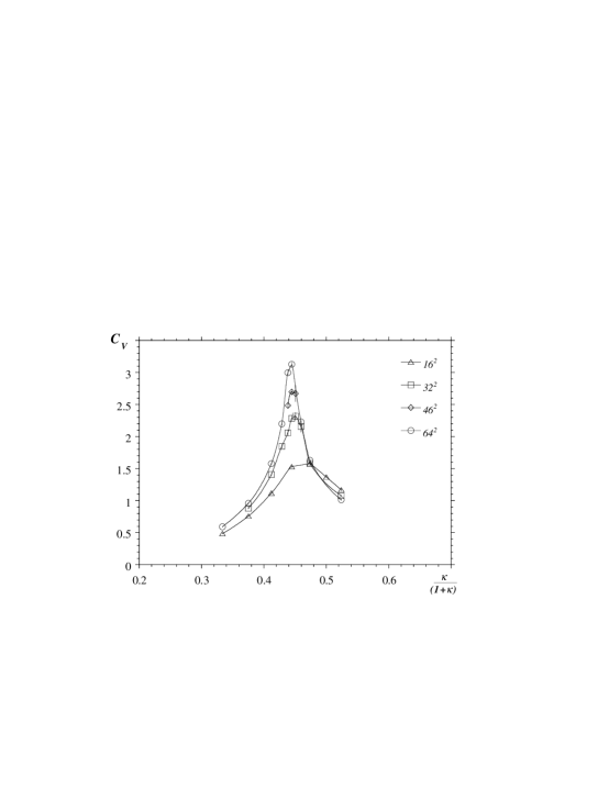
Figure 14: Plot of the specific heat observable [38]. The growth of the specific heat peak with system size indicates a continuous transition.

Further evidence for the crumpling transition being continuous is provided by numerical simulations [39, 40, 41, 42, 43, 44, 45, 46, 47, 38] where the analysis of observables like the specific heat (see Fig.14) or the radius of gyration radius give textbook continuous phase transitions, although the precise value of the exponents at the transition are difficult to pin down. Since this model has also been explored numerically with different discretizations on several lattices, there is clear evidence for universality of the crumpling transition [46], again consistent with a continuous transition. In Appendix C we present more details of suitable discretizations of the energy for numerical simulations of membranes.

4.1.3 The Flat Phase

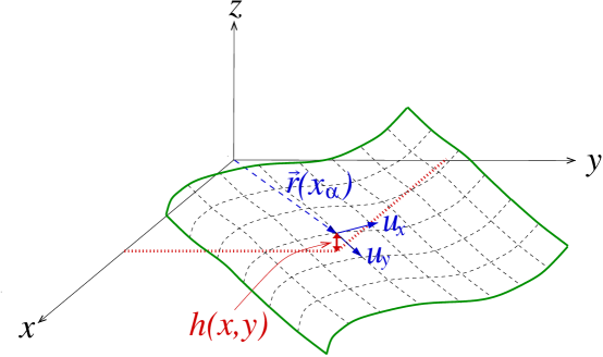
Figure 15: Coordinates for fluctuations in the flat phase

In a flat membrane (see Fig.15), we consider the strain tensor

$$u_{\alpha\beta}=\partial_{\alpha}u_{\beta}+\partial_{\beta}u_{\alpha}+\partial_{\alpha}h\partial_{\beta}h\ .$$ (19)

The free energy Eq.(7) becomes

$$F({\bf u},h)=\int d^{D}{\bf x}\left[\frac{\hat{\kappa}}{2}(\partial_{\alpha}\partial_{\beta}h)^{2}+\mu u_{\alpha\beta}u^{\alpha\beta}+\frac{\lambda}{2}(u^{\alpha}_{\alpha})^{2}\right]\ ,$$ (20)

where we have dropped irrelevant terms. One recognizes the standard Landau Free energy of elasticity theory, with Lamé coefficients $\mu$ and $\lambda$, plus an extrinsic curvature term, with bending rigidity $\hat{\kappa}$. These couplings are related to the original ones in Eq.(7) by $\mu=u\zeta^{4-D}$, $\lambda=2v\zeta^{4-D}$, $\hat{\kappa}=\kappa\zeta^{4-D}$ and $t=-4(\mu+\frac{D}{2}\lambda)\zeta^{D-2}$.

The large distance properties of the flat phase for crystalline membranes are completely described by the Free energy Eq.(20). Since the bending rigidity may be scaled out at the crumpling transition, the free energy becomes a function of $\frac{\mu}{\kappa^{2}}$ and $\frac{\lambda}{\kappa^{2}}$. The $\beta$-function for the couplings $u,v$ at $\kappa=1$ may be calculated within an $\varepsilon$-expansion, which we describe in detail in Appendix E. Let us recall that the dependence on $\kappa$ may be trivially restored at any stage. The result is

$$\beta_{\mu}(\mu_{R},\lambda_{R}) = -\varepsilon\mu_{R}+\frac{\mu_{R}^{2}}{8\pi^{2}}(\frac{d_{c}}{3}+20A)$$ (21)

$$\beta_{\lambda}(\mu_{R},\lambda_{R}) = -\varepsilon\lambda_{R}+\frac{1}{8\pi^{2}}(\frac{d_{c}}{3}\mu^{2}_{R}+2(d_{c}+10A)\lambda_{R}\mu_{R}+2d_{c}\lambda^{2}_{R})\ ,$$

where $d_{c}=d-D$, and $A=\frac{\mu_{R}+\lambda_{R}}{2\mu_{R}+\lambda_{R}}$. These $\beta$ functions show four fixed points whose actual values are shown in Table 1.

Figure 16: Phase diagram for the phantom flat phase. There are three infra-red unstable FPs, labelled by FLP1, FLP2 and FLP3, but the physics of the flat phase is governed by the infra-red stable FP (FLFP).

As apparent from Fig.16, the phase diagram of the flat phase turns out to be slightly more involved than the one shown in Fig.13, as there are three FPs in addition to the FLFP already introduced. These additional FPs are infra-red unstable, however, and can only be reached for very specific values of the Lamé coefficients, so for any practical situation we can regard the FLFP as the only existing FP in the flat phase.

FP $\mu^{\ast}_{R}$ $\lambda_{R}^{\ast}$ $\eta$ $\eta_{u}$ FP1 $0$ $0$ $0$ $0$ FP2 $0$ $2\varepsilon/d_{c}$ $0$ $0$ FP3 $\frac{12\varepsilon}{20+d_{c}}$ $\frac{-6\varepsilon}{20+d_{c}}$ $\frac{\varepsilon}{2+d_{c}/10}$ $\frac{\varepsilon}{1+20/d_{c}}$ FLFP $\frac{12\varepsilon}{24+d_{c}}$ $\frac{-4\varepsilon}{24+d_{c}}$ $\frac{\varepsilon}{2+d_{c}/12}$ $\frac{\varepsilon}{1+24/d_{c}}$

Table 1: The FPs and critical exponents of the flat phase.

The properties of the flat phase

The flat phase is a very important phase as will be apparent once we study the full model, including self-avoidance. For that reason we turn now to a more detailed study of its most important properties.

Fig.11 (c) gives an intuitive visualization of a crystalline membrane in the flat phase. The membrane is essentially a flat two dimensional object up to fluctuations in the perpendicular direction. The rotational symmetry of the model is spontaneously broken, being reduced from $O(d)$ to $O(d-D)\times O(D)$. The remnant rotational symmetry is realized in Eq.(20) as

$$h_{i}({\bf x}) \rightarrow h_{i}({\bf x})+A^{i\alpha}{\bf x}_{\alpha}$$ (22)

$$u_{\alpha}({\bf x}) \rightarrow u_{\alpha}-A^{i\alpha}h_{i}-\frac{1}{2}\delta^{ij}(A^{i\alpha}A^{\beta j}{\bf x}_{\beta})\ ,$$

where $A^{i\alpha}$ is a $D\times(d-D)$ matrix. This relation is very important as it provides Ward identities which simplify enormously the renormalization of the theory.

Let us first study the critical exponents of the model. There are two key correlators, involving the in-plane and the out-of-plane phonon modes. Using the RG equations, it is easy to realize that at any given FP, the low-$p$ limit of the model is given by

$$\Gamma_{uu}({\vec{p}}) \sim |{\vec{p}}|^{2+\eta_{u}}$$ (23)

$$\Gamma_{hh}({\vec{p}}) \equiv |{\vec{p}}|^{4}\kappa({\vec{p}})\sim|{\vec{p}}|^{4-\eta}\ ,$$

where the last equation defines the anomalous elasticity $\kappa({\vec{p}})$ as a function of momenta ${\vec{p}}$. These two exponents are not independent, since they satisfy the scaling relation [53]

$$\eta_{u}=4-D-2\eta\ ,$$ (24)

which follows from the Ward identities associated with the remnant rotational symmetry (Eqn.(22). Another important exponent is the roughness exponent $\zeta$, which measures the fluctuations transverse to the flat directions. It can be expressed as $\zeta=\frac{4-D-\eta}{2}$.

The long wavelength properties of the flat phase are described by the FLFP (see Fig.16). Since the FLFP occurs at non-zero renormalized values of the Lamé coefficients, the associated critical exponents discussed earlier are clearly non-Gaussian. Within an $\varepsilon$-expansion, the values for the critical exponents are given in Table 1. There are alternative estimates available from different methods. These are

• Numerical Simulation: In [38] a large scale simulation of the model was performed using very large meshes. The results obtained for the critical exponents are very reliable, namely

  $$\begin{array}[]{l l l}\eta_{u}=0.50(1)&\eta=0.750(5)&\zeta=0.64(2)\end{array}$$ (25)

  For a review of numerical results see [48, 49].

• SCSA Approximation: This consists of suitably truncating the Schwinger-Dyson equations to include up to four-point correlation functions [51]. The result for general $d$ is

  $$\eta(d)=\frac{4}{d_{c}+(16-2d_{c}+d^{2}_{c})^{1/2}}\ ,$$ (26)

  which for $d=3$ gives

  $$\begin{array}[]{l l l}\eta_{u}=0.358&\eta=0.821&\zeta=0.59\end{array}$$ (27)

• Large d expansion: The result is [50]

  $$\eta=\frac{2}{d}\rightarrow\eta(3)=2/3$$ (28)

We regard the results of the numerical simulation as our most accurate estimates, since we can estimate the errors. The results obtained from the SCSA, which are the best analytical estimate, are in acceptable agreement with simulations.

Finally there are two experimental measurements of critical exponents for the flat phase of crystalline membranes. The static structure factor of the red blood cell cytoskeleton (see Sect.1) has been measured by small-angle x-ray and light scattering, yielding a roughness exponent of $\zeta=0.65(10)$ [13]. Freeze-fracture electron microscopy and static light scattering of the conformations of graphitic oxide sheets (Sect.1) revealed flat sheets with a fractal dimension $d_{H}=2.15(6)$. Both these values are in good agreement with the best analytic and numerical predictions, but the errors are still too large to discriminate between different analytic calculations.

The Poisson ratio of a crystalline membrane (measuring the transverse elongation due to a longitudinal stress [54]) is universal and within the SCSA approximation, which we regard as the more accurate analytical estimate, is given by

$$\sigma(D)=-\frac{1}{D+1}\rightarrow\sigma(2)=-1/3\ ,$$ (29)

This result has been accurately checked in numerical simulations [55]. Rather remarkably, it turns out to be negative. Materials having a negative Poisson ratio are called auxetic. This highlights potential applications of crystalline membranes to materials science since auxetic materials have a wide variety of potential applications as gaskets, seals etc.

Finally another critical regime of a flat membrane is achieved by subjecting the membrane to external tension [56, 57]. This allows a low temperature phase in which the membrane has a domain structure, with distinct domains corresponding to flat phases with different bulk orientations. This describes, physically, a buckled membrane whose equilibrium shape is no longer planar.

4.2 Self-avoiding

Self-avoidance is a necessary interaction in any realistic description of a crystalline membrane. It is introduced in the form of a delta-function repulsion in the full model Eq.(5). We have already analyzed the phantom case and explored in detail the distinct phases. The question before us now is the effect of self-avoidance on each of these phases.

The first phase we analyze is the flat phase. Since self-intersections are unlikely in this phase, it is intuitively clear that self-avoidance should be irrelevant. This may also be seen if one neglects the effects of the in-plane phonons. In the self-avoiding term for the flat phase we have

$$\frac{b}{2}\int d^{D}{\bf x}\,d^{D}{\bf y}\delta^{d}({\vec{r}}({\bf x})-{\vec{r}}({\bf y}))$$

$$= \frac{b}{2}\int d^{D}{\bf x}\,d^{D}{\bf y}\delta^{D}(\zeta({\bf x}-{\bf y})+{\bf u}({\bf x})-{\bf u}({\bf y}))\delta^{d-D}(h({\bf x})-h({\bf y}))$$

$$\sim \frac{b}{2}\int d^{D}{\bf x}\,d^{D}{\bf y}\delta^{D}(\zeta({\bf x}-{\bf y}))\delta^{d-D}(h({\bf x})-h({\bf y}))=0\ ,$$

as the trivial contribution where the membrane equals itself is eliminated by regularization. The previous argument receives additional support from numerical simulations in the flat phase, where it is found that self-intersections are extremely rare in the typical configurations appearing in those simulations. It seems clear that self-avoidance is most likely an irrelevant operator, in the RG sense, of the FLFP. Nevertheless, it would be very interesting if one could provide a more rigorous analytical proof for this statement. A rough argument can be made as follows. Shortly we will see that the Flory approximation for self-avoiding membranes predicts a fractal dimension $d_{H}=2.5$. For bulk dimension $d$ exceeding 2.5 therefore we expect self-avoidance to be irrelevant. A rigorous proof of this sort remains rather elusive, as it involves the incorporation of both self-avoidance and non-linear elasticity, and this remains a difficult open problem.

The addition of self-avoidance in the crumpled phase consists of adding the self-avoiding interaction to the free energy of Eq.(10)

$$F({\vec{r}})=\frac{1}{2}\int d^{D}{\bf x}(\partial_{\alpha}{\vec{r}}({\bf x}))^{2}+\frac{b}{2}\int d^{D}{\bf x}\,d^{D}{\bf y}\delta^{d}({\vec{r}}({\bf x})-{\vec{r}}({\bf y}))\ ,$$ (31)

which becomes the natural generalization of the Edwards’ model for polymers to $D$-dimensional objects. Standard power counting shows that the GFP of the crumpled phase is infra-red unstable to the self-avoiding perturbation for

$$\varepsilon(D,d)\equiv 2D-d\frac{2-D}{2}>0\ ,$$ (32)

which implies that self-avoidance is a relevant perturbation for $D=2$-objects at any embedding dimension $d$. The previous remarks make it apparent that it is possible to perform an $\varepsilon$-expansion of the model [58, 59, 60, 61]. In Appendix F, we present the calculation of the $\beta$-function at lowest order in $\varepsilon$ using the MOPE (Multi-local-operator-product-expansion) formalism [62, 63]. The MOPE formalism has the advantage that it is more easily generalizable to higher orders in $\varepsilon$, and enables concrete proofs showing that the expansion may be carried out to all orders. At lowest order, the result for the $\beta$-function is

$$\beta_{b}(b_{R}) = -\varepsilon b_{R}+\frac{(2-D)^{-1+\frac{d}{2}}}{(4\pi)^{\frac{d}{2}}}\left(\frac{2\pi^{\frac{D}{2}}}{\Gamma(D/2)}\right)^{2+\frac{d}{2}}\left[\frac{\Gamma(\frac{D}{2-D})^{2}}{\Gamma(\frac{2D}{2-D})}+\frac{d}{2}\frac{(2-D)^{2}}{2D}\right]\frac{b^{2}_{R}}{2}$$ (33)

$$\equiv -\varepsilon b_{R}+a_{1}b_{R}^{2}\ .$$

The infra-red stable FP is given at lowest order in $\varepsilon$ by $b^{\ast}_{R}=\frac{\varepsilon}{a_{1}}$, which clearly shows that the GFP of the crumpled phase is infra-red unstable in the presence of self-avoidance.

The preceding results are shown in Fig.17 and may be summarized as

• The flat phase of self-avoiding crystalline membranes is exactly the same as the flat phase of phantom crystalline tethered membranes.

• The crumpled phase of crystalline membranes is destabilized by the presence of any amount of self-avoidance.

Figure 17: The addition of Self-avoidance at the Crumpled and Flat phases.

The next issue to elucidate is whether this new SAFP describes a crumpled self-avoiding phase or a flat one and to give a more quantitative description of the critical exponents describing the universality class. Supposing that the SAFP is, in fact, flat we must understand its relation to the FLFP describing the physics of the flat phase and the putative phase transitions between these two.

4.2.1 The nature of the SAFP

Let us study in more detail the model described in Eq.(31). The key issue is whether this model still admits a crumpled phase, and if so to determine the associated size exponent. On general grounds we expect that there is a critical dimension $d_{c}$, below which there is no crumpled phase (see Fig.18).

Figure 18: The size exponent as a function of $d$. There is a critical dimension $d_{c}$ below which the crumpled phase disappears.

An estimate for the critical dimension may be obtained from a Flory approximation in which minimizes the free energy obtained by replacing both the elastic and self-avoiding terms with the radius of gyration raised to the power of the appropriate scaling dimensions. Within the Flory treatment a $D$-dimensional membrane is in a crumpled phase, with a size exponent given by

$$\nu=(D+2)/(d+2)\ .$$ (34)

From this it follows that $d_{c}=D$ (see Fig.18). The Flory approximation, though very accurate for polymers ($D=1$), remains an uncontrolled approximation.

In contrast the $\varepsilon$-expansion provides a systematic determination of the critical exponents. For the case of membranes, however, some extrapolation is required, as the upper critical dimension is infinite. This was done in [64], where it is shown that reconsidering the $\varepsilon$-expansion as a double expansion in $\varepsilon$ and $D$, critical quantities may be extrapolated for $D=2$-dimensional objects. At lowest order in $\varepsilon$, the membrane is in a crumpled phase. The enormous task of calculating the next correction ($\varepsilon^{2}$) was successfully carried out in [65], employing more elaborate extrapolation methods than those in [64]. Within this calculation, the $d=3$ membrane is still in a crumpled phase, but with a size exponent now closer to 1. It cannot be ruled out that the $\varepsilon$-expansion, successfully carried out to all orders could give a flat phase $\nu=1$. In fact, the authors in [65, 66] present some arguments in favor of a scenario of this type, with a critical dimension $d_{c}\sim 4$.

Other approaches have been developed with different results. A Gaussian approximation was developed in [67, 68]. The size exponent of a self-avoiding membrane within this approach is

$$\nu=4/d,$$ (35)

and since one has $\nu>1$ for $d\leq 4$, one may conclude that the membrane is flat for $d\leq d_{c}=4$. Since we cannot determine the accuracy of the Gaussian approximation this estimate must be viewed largely as interesting speculation. Slightly more elaborate arguments of this type [8] yield an estimated critical dimension $d_{c}=3$.

Numerical simulations

We have seen that numerical simulations provide good support for analytic results in the case of phantom membranes. When self-avoidance is included, numerical simulations become invaluable, since analytic results are harder to come by. It is for this reason that we discuss them in greater detail than in previous sections.

A possible discretization of membranes with excluded volume effects consists of a network of $N$ particles arranged in a triangular array. Nearest neighbors interact with a potential

$$V_{NN}({\vec{r}})=\left\{\begin{array}[]{c c}0&\mbox{for $|{\vec{r}}|<b$ }\\ \infty&\mbox{for $|{\vec{r}}|>b$}\end{array}\right.\ ,$$ (36)

although some authors prefer a smoothened version, with the same general features. The quantity $b$ is of the order of a few lattice spacings. This is a lattice version of the elastic term in Eq.(31). The discretization of the self-avoidance is introduced as a repulsive hard sphere potential, now acting between any two atoms in the membrane, instead of only nearest neighbors. A hard sphere repulsive potential is, for example,

$$V_{Exc}({\vec{r}})=\left\{\begin{array}[]{c c}\infty&\mbox{for $|{\vec{r}}|<\sigma$}\\ 0&\mbox{ for $|{\vec{r}}|>\sigma$ }\end{array}\right.\ ,$$ (37)

where $\sigma$ is the range of the potential, and $\sigma<b$. Again, some smoothened versions, continuous at $|{\vec{r}}|=\sigma$, have also been considered. This model may be pictured as springs, defined by the nearest-neighbor potential Eq.(36), with excluded volume effects enforced by balls of radius $\sigma$ (Eq.(37)). This model represents a lattice discretization of Eq.(31).

Early simulations of this type of model [39, 40] provided a first estimate of the size exponent at $d=3$ fully compatible with the Flory estimate Eq.(34). The lattices examined were not very large, however, and subsequent simulations with larger volumes [69, 70] found that the $d=3$ membrane is actually flat. This result is even more remarkable if one recalls that there is no explicit bending rigidity.

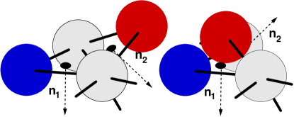
Figure 19: Visualization of bending rigidity generated by a hard sphere potential. Normals ${\vec{n}}_{1}$ and ${\vec{n}}_{2}$ cannot be anti-parallel.

The flat phase was a very surprising result, in some conflict with the insight provided from the analytical estimates discussed in the previous subsection. An explanation for it came from the observation [71] that excluded volume effects induce bending rigidity, as depicted in Fig.19. The reason is that the excluded volume effects generate a non-zero expectation value for the bending rigidity, since the normals can be parallel, but not anti-parallel (see 19). This induced bending rigidity was estimated and found to be big enough to drive the self-avoiding membrane well within the flat phase of the phantom one. This means that this particular discretization of the model renders any potential SAFP inaccessible and the physics is described by the FLFP. In [72] the structure function of the self-avoiding model is numerically computed and found to compare well with the analytical structure function for the flat phase of phantom crystalline membranes, including comparable roughness exponents.

The natural question then to ask is whether it is possible to reduce the bending rigidity sufficiently to produce a crumpled self-avoiding phase. Subsequent studies addressed this issue in various ways. The most natural way is obviously to reduce the range of the potential sufficiently that the induced bending rigidity is within the crumpled phase. This is the approach followed in [73]. The flat phase was found to persist to very small values of $\sigma$, with eventual signs of a crumpled phase. This crumpled phase may essentially be due to the elimination at self-avoidance at sufficiently small $\sigma$. A more comprehensive study, in which the same limit is performed this time with an excluded volume potential which is a function of the internal distance along the lattice [74], concluded that for large membranes, inclusion of excluded volume effects, no matter how small, leads to flatness. A different approach to weakening the flat phase, bond dilution [75], found that the flat phase persists until the percolation critical point. In conclusion the bulk of accumulated evidence indicates that flatness is an intrinsic consequence of self-avoidance. If this is indeed correct the SAFP coincides with FLFP and this feature is an inherent consequence of self-avoidance, rather than an artifact of discretization.

Given the difficulties of finding a crumpled phase with a repulsive potential, simulations for larger values of the embedding space dimension $d$ have also been performed [76, 77]. These simulations show clear evidence that the membrane remains flat for $d=3$ and $4$ and undergoes a crumpling transition for $d\geq 5$, implying $d_{c}\geq 4$.

An alternative approach to incorporating excluded volume effects corresponds to discretize a surface with a triangular lattice and imposing the self-avoidance constraint by preventing the triangular plaquettes from inter-penetrating. This model has the advantage that is extremely flexible, since there is no restriction on the bending angle of adjacent plaquettes (triangles) and therefore no induced bending rigidity (see C).

The first simulations of the plaquette model [78] found a size exponent in agreement with the Flory estimate Eq. 34. A subsequent simulation [79] disproved this result, and found a size exponent $\nu=0.87$, higher than the Flory estimate, but below one. More recent results using larger lattices and more sophisticated algorithms seem to agree completely with the results obtained from the ball and spring models [80].

Further insight into the lack of a crumpled phase for self-avoiding crystalline membranes is found in the study of folding [81, 82, 83, 84, 85, 86, 87]. This corresponds to the limit of infinite elastic constants studied by David and Guitter with the further approximation that the space of bending angles is discretized. One quickly discovers that the reflection symmetries of the allowed folding vertices forbid local folding (crumpling) of surfaces. There is therefore essentially no entropy for crumpling. There is, however, local unfolding and the resulting statistical mechanical models are non-trivial. The lack of local folding is the discrete equivalent of the long-range curvature-curvature interactions that stabilize the flat phase. The dual effect of the integrity of the surface (time-independent connectivity) and self-avoidance is so powerful that crumpling seems to be impossible in low embedding dimensions.

4.2.2 Attractive potentials

Self-avoidance, as introduced in Eq.(37) is a totally repulsive force among monomers. There is the interesting possibility of allowing for attractive potentials also. This was pioneered in [71] as a way to escape to the induced bending rigidity argument (see Fig.19), since an attractive potential would correspond to a negligible (or rather a negative) bending rigidity. Remarkably, in [71], a compact (more crumpled) self-avoiding phase was found, with fractal dimension close to 3.

This was further studied in [88], where it was found that with an attractive Van der Waals potential, the crystalline membrane underwent a sequence of folding transitions leading to a crumpled phase. In [89] similar results were found, but instead of a sequence of folding transitions a crumpled phase was found with an additional compact (more crumpled phase) at even lower temperatures. Subsequent work gave some support to this scenario [90].

On the analytical side, the nature of the $\Theta$-point for membranes and its relevance to the issue of attractive interactions has been addressed in [91].

We think that the study of a tether with an attractive potential remains an open question begging for new insights. A thorough understanding of the nature of the compact phases produced by attractive interactions would be of great value.

4.2.3 The properties of the SAFP

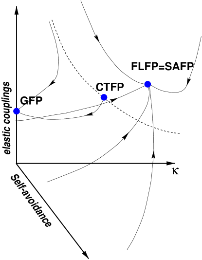
Figure 20: The conjectured phase diagram for self-avoiding crystalline membranes in $d=3$. With any degree of self-avoidance the flows are to the flat phase fixed point of the phantom model (FLFP).

The enormous efforts dedicated to study the SAFP have not resulted in a complete clarification of the overall scenario since the existing analytical tools do not provide a clear picture. Numerical results clearly provide the best insight. For the physically relevant case $d=3$, the most plausible situation is that there is no crumpled phase and that the flat phase is identical to the flat phase of the phantom model. For example, the roughness exponents $\zeta_{SA}$ from numerical simulations of self-avoidance at $d=3$ using ball-and-spring models [76] and the roughness exponent at the FLFP, Eq.(25), compare extremely well

$$\zeta_{SA}=0.64(4)\ ,\ \zeta=0.64(2)\ ,$$ (38)

So the numerical evidence allows us to conjecture that the SAFP is exactly the same as the FLFP, and that the crumpled self-avoiding phase is absent in the presence of purely repulsive potentials (see Fig.20). This identification of fixed points enhances the significance of the FLFP treated earlier. It would be very helpful if analytical tools were developed to further substantiate this statement.

5 Anisotropic Membranes

An anisotropic membrane is a crystalline membrane having the property that the elastic or the bending rigidity properties in one distinguished direction are different from those in the $D-1$ remaining directions. As for the isotropic case we keep the discussion general and describe the membrane by a $d$-dimensional ${\vec{r}}({\bf x}_{\perp},y)$, where now the $D$ dimensional coordinates are split into $D-1\ \ {\bf x}_{\perp}$ coordinates and the orthogonal distinguished direction $y$.

The construction of the Landau free energy follows the same steps as in the isotropic case. Imposing translational invariance, $O(d)$ rotations in the embedding space and $O(D-1)$ rotations in internal space, the equivalent of Eq.(5) is now

$$F(\vec{r}({\bf x})) = \frac{1}{2}\int d^{D-1}{\bf x}_{\perp}dy\left[\kappa_{\perp}(\partial_{\perp}^{2}\vec{r})^{2}+\kappa_{y}(\partial_{y}^{2}\vec{r})^{2}\right.$$ (39)

$$+\kappa_{\perp y}\partial_{y}^{2}\vec{r}\cdot\partial_{\perp}^{2}\vec{r}+t_{\perp}(\partial_{\alpha}^{\perp}\vec{r})^{2}+t_{y}(\partial_{y}\vec{r})^{2}$$

$$+\frac{u_{\perp\perp}}{2}(\partial_{\alpha}^{\perp}\vec{r}\cdot\partial_{\beta}^{\perp}\vec{r})^{2}+\frac{u_{yy}}{2}(\partial_{y}\vec{r}\cdot\partial_{y}\vec{r})^{2}$$

$$+u_{\perp y}(\partial_{\alpha}^{\perp}\vec{r}\cdot\partial_{y}\vec{r})^{2}+\frac{v_{\perp\perp}}{2}(\partial_{\alpha}^{\perp}\vec{r}\cdot\partial_{\alpha}^{\perp}\vec{r})^{2}$$

$$\left.+v_{\perp y}(\partial_{\alpha}^{\perp}\vec{r})^{2}(\partial_{y}\vec{r})^{2}\right]$$

$$+\frac{b}{2}\int d^{D}{\bf x}\int d^{D}{\bf x}^{\prime}\delta^{d}(\vec{r}({\bf x})-\vec{r}({\bf x}^{\prime})).$$

This model has eleven parameters, representing distinct physical interactions:

• $\kappa_{\perp},\kappa_{y},\kappa_{\perp y}$ bending rigidity: the anisotropic versions of the isotropic bending rigidity splits into three distinct terms.

• $t_{\perp},t_{y},u_{\perp\perp},u_{yy},v_{\perp\perp},v_{\perp y}$ elastic constants: there are six quantities describing the microscopic elastic properties of the anisotropic membrane.

• $b$, self-avoidance coupling: This particular term is identical to its isotropic counterpart.

Following the same steps as in the isotropic case, we split

$${\vec{r}}({\bf x})=(\zeta_{\perp}{\bf x}_{\perp}+{\bf u}_{\perp}({\bf x}),\zeta_{y}y+u_{y}({\bf x}),h({\bf x}))\ ,$$ (40)

with ${\bf u}_{\perp}$ being the $D-1$-dimensional phonon in-plane modes, $u_{y}$ the in-plane phonon mode in the distinguished direction $y$ and $h$ the $d-D$ out-of-plane fluctuations. If $\zeta_{\perp}=\zeta_{y}=0$, the membrane is in a crumpled phase and if both $\zeta_{\perp}\neq 0$ and $\zeta_{y}\neq 0$ the membrane is in a flat phase very similar to the isotropic case (how similar will be discussed shortly). There is, however, the possibility that $\zeta_{\perp}=0$ and $\zeta_{y}\neq 0$ or $\zeta_{\perp}\neq 0$ and $\zeta_{y}=0$. This describes a completely new phase, in which the membrane is crumpled in some internal directions but flat in the remaining ones. A phase of this type is called a tubular phase and does not appear when studying isotropic membranes. In Fig.21 we show an intuitive visualization of a tubular phase along with the corresponding flat and crumpled phases of anisotropic membranes.

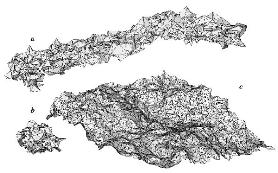
Figure 21: Examples of a) the tubular phase b) the crumpled phase and c) the flat phase of an anisotropic phantom crystalline membrane taken from the simulations of [92]

We will start by studying the phantom case. We show, using both analytical and numerical arguments, that the phase diagram contains a crumpled, tubular and flat phase. The crumpled and flat phases are equivalent to the isotropic ones, so anisotropy turns out to be an irrelevant interaction in those phases. The new physics is contained in the tubular phase, which we describe in detail, both with and without self-avoidance.

5.1 Phantom

5.1.1 The Phase diagram

We first describe the mean field theory phase diagram and then the effect of fluctuations. There are two situations depending on the particular values of the function $\Delta$, which depends on the elastic constants $u_{\perp\perp},v_{\perp y},u_{yy}$ and $v_{\perp\perp}$. Since the derivation is rather technical, we refer to Appendix G for the details.

• Case A ($\Delta>0$): the mean field solution displays all possible phases. When $t_{y}>0$ and $t_{\perp}>0$ the model is in a crumpled phase. Lowering the temperature, one of the $t$ couplings becomes negative, and we reach a tubular phase (either $\perp$ or $y$-tubule). A further reduction of the temperature eventually leads to a flat phase.

• Case B ($\Delta<0$): in this case the flat phase disappears from the mean field solution. Lowering further the temperature leads to a continuous transition from the crumpled phase to a tubular phase. Tubular phases are the low temperature stable phases in this regime.

This mean field result is summarized in Fig.22.

Figure 22: The phase diagram for anisotropic phantom membranes

Beyond mean field theory, the Ginsburg criterion applied to this model tells us that the phase diagram should be stable for physical membranes $D=2$ at any embedding dimension $d$, so the mean field scenario should give the right qualitative picture for the full model.

Numerical simulations have spectacularly confirmed this result. We have already shown in Fig.21 the results from the numerical simulation in [92], where it was shown that changing the temperature generates a sequence of transitions crumpled-to-tubular and tubular-to-flat, in total agreement with case A) in the mean field result illustrated in Fig.22.

We now turn to a more detailed study of both the crumpled and flat anisotropic phases. Since we have already studied crumpled and flat phases we just outline how those are modified when anisotropy is introduced.

5.1.2 The Crumpled Anisotropic Phase

In this phase $t_{y}>0$ and $t_{\perp}>0$, and the free energy Eq.(39) reduces for $D\geq 2$ to

$$F(\vec{r}({\bf x}))=\frac{1}{2}\int d^{D-1}{\bf x}_{\perp}dy\left[t_{\perp}(\partial_{\alpha}^{\perp}\vec{r})^{2}+t_{y}(\partial_{y}\vec{r})^{2}\right]+\mbox{Irrelevant}\ .$$ (41)

By redefining the $y$ direction as $y^{\prime}=\frac{t_{\perp}}{t_{y}}y$ this reduces to Eq.(10), with $t\equiv t_{\perp}$. We have proved that anisotropy is totally irrelevant in this particular phase.

5.1.3 The Flat Phase

This phase becomes equivalent to the isotropic case as well. Intuitively, this may be obtained from the fact that if the membrane is flat, the intrinsic anisotropies are only apparent at short-distances, and therefore by analyzing the RG flow at larger and larger distances the membrane should become isotropic. This argument may be made slightly more precise [93].

5.2 The Tubular Phase

We now turn to the study of the novel tubular phase, both in the phantom case and with self-avoidance. Since the physically relevant case for membranes is $D=2$ the $y$-tubular and $\perp$-tubular phase are the same. So we concentrate on the properties of the $y$-tubular phase.

The key critical exponents characterizing the tubular phase are the size (or Flory) exponent $\nu$, giving the scaling of the tubular diameter $R_{g}$ with the extended ($L_{y}$) and transverse ($L_{\perp}$) sizes of the membrane, and the roughness exponent $\zeta$ associated with the growth of height fluctuations $h_{rms}$ (see Fig.23):

$$R_{g}(L_{\perp},L_{y}) \propto L_{\perp}^{\nu}S_{R}(L_{y}/L_{\perp}^{z})$$ (42)

$$h_{rms}(L_{\perp},L_{y}) \propto L_{y}^{\zeta}S_{h}(L_{y}/L_{\perp}^{z})$$

Here $S_{R}$ and $S_{h}$ are scaling functions [94, 95] and $z$ is the anisotropy exponent.

Figure 23: A schematic illustration of a tubular configuration indicating the radius of gyration $R_{g}$ and the height fluctuations $h_{rms}$.

The general free energy described in Eq.(39) may be simplified considerably in a $y$-tubular phase. The analysis required is involved and we refer the interested reader to [96, 97]. We just quote the final result. It is

$$F(u,\vec{h}) = \frac{1}{2}\int d^{D-1}{\bf x}_{\perp}dy\left[\kappa(\partial_{y}^{2}\vec{h})^{2}+t(\partial_{\alpha}\vec{h})^{2}\right.$$ (43)

$$+g_{\perp}(\partial_{\alpha}u+\partial_{\alpha}\vec{h}\partial_{y}\vec{h})^{2}$$

$$+\left.g_{y}(\partial_{y}u+\frac{1}{2}(\partial_{y}\vec{h})^{2})^{2}\right]$$

$$+\frac{b}{2}\int dyd^{D-1}{\bf x}_{\perp}d^{D-1}{\bf x}_{\perp}^{\prime}\delta^{d-1}(\vec{h}({\bf x}_{\perp},y)-\vec{h}({\bf x}_{\perp}^{\prime},y))\ .$$

Comparing with Eq.(39), this free energy does represent a simplification as the number of couplings has been reduced from eleven to five. Furthermore, the coupling $g_{\perp}$ is irrelevant by standard power counting. The most natural assumption is to set it to zero. In that case the phase diagram one obtains is shown in Fig.24. Without self-avoidance $b=0$, the Gaussian Fixed Point (GFP) is unstable and the infra-red stable FP is the tubular phase FP (TPFP). Any amount of self-avoidance, however, leads to a new FP, the Self-avoiding Tubular FP (SAFP), which describes the large distance properties of self-avoiding tubules.

Figure 24: The phase diagram for self-avoiding anisotropic membranes with the Gaussian fixed point (GFP), the tubular phase fixed point (TPFP) and the self-avoidance fixed point (SAFP).

We just mention, though, that other authors advocate a different scenario [95]. For sufficiently small embedding dimensions $d$, including the physical $d=3$ case, these authors suggest the existence of a new bending rigidity renormalized FP (BRFP), which is the infra-red FP describing the actual properties of self-avoiding tubules (see Fig. 25).

Figure 25: The phase diagram for self-avoiding anisotropic membranes with the Gaussian fixed point (GFP), the tubular phase fixed point (TPFP), the self-avoidance fixed point (SAFP) and the bending rigidity fixed point (BRFP).

Here we follow the arguments presented in [97] and consider the model defined by Eq.(43) with the $g_{\perp}$-term as the model describing the large distance properties of tubules. One can prove then than there are some general scaling relations among the critical exponents. All three exponents may be expressed in terms of a single exponent

$$\zeta = \frac{3}{2}+\frac{1-D}{2z}$$ (44)

$$\nu =\zeta z\ .$$

Remarkably, the phantom case as described by Eq.(43) can be solved exactly. The result for the size exponent is

$$\nu_{Phantom}(D)=\frac{5-2D}{4}\ ,\nu_{Phantom}(2)=\frac{1}{4}$$ (45)

with the remaining exponents following from the scaling relations Eq.(44).

$d$ $\nu$ $\nu_{F}$ $\nu_{V}$ $\nu_{Flory}$ 8 $0.333(5)$ $0.34(1)$ $0.34(1)$ $0.333$ 7 $0.374(8)$ $0.39(2)$ $0.39(2)$ $0.375$ 6 $0.42(1)$ $0.44(2)$ $0.44(4)$ $0.429$ 5 $0.47(1)$ $0.51(3)$ $0.51(5)$ $0.500$ 4 $0.54(2)$ $0.60(4)$ $0.60(6)$ $0.600$ 3 $0.62(2)$ $0.71(6)$ $0.70(9)$ $0.750$

Table 2: Different extrapolations for the size exponent at different embedding dimensions $d$ [97]. The first column gives the corrections to the mean field result, the second corrections to the Flory estimate and the third corresponds to corrections to the Gaussian approximation. The last column quotes the Flory estimate for comparison.

The self-avoiding case may be treated with techniques similar to those in isotropic case. The size exponent may be estimated within a Flory approach. The result is

$$\nu_{Flory}=\frac{D+1}{d+1}\ .$$ (46)

The Flory estimate is an uncontrolled approximation. Fortunately, a $\varepsilon$-expansion, adapting the MOPE technique described for the self-avoiding isotropic case to the case of tubules, is also possible [96, 97]. The $\beta$-functions are computed and provide evidence for the phase diagram shown in Fig.24. Using rather involved extrapolation techniques, it is possible to obtain estimates for the size exponent, which are shown in Table 2. The rest of the exponents may be computed from the scaling relations.

6 Defects in membranes: The Crystalline-Fluid transition and Fluid membranes

A flat crystal melts into a liquid when the temperature is increased. This transition may be driven by the sequential liberation of defects, as predicted by the KTNHY theory. The KTNHY theory is schematically shown in Fig.26. With increasing temperature, a crystal melts first to an intermediate hexatic phase via a continuous transition, and finally goes to a conventional isotropic fluid phase via another continuous transition.

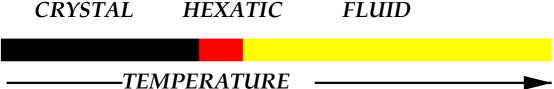
Figure 26: Two stage melting according to KTNHY theory.

We will not review here either the KTNHY theory or the experimental evidence in its favor – [98]. We just want to emphasize here that the KTNHY theory is in general agreement with existing experiments, although there are two main points worth keeping in mind when studying the more difficult case of fluctuating geometries. 1) The experimental evidence for the existence of the hexatic phase is not completely settled in those transitions which are continuous. 2) Some 2D crystals (like Xenon absorbed on graphite) melt to a fluid phase via a first order transition without any intermediate hexatic phase.

The straight-forward translation of the previous results to the tethered membrane would suggest a similar scenario. There would then be a crystalline to hexatic transition and a hexatic to fluid transition, as schematically depicted in Fig.26. Although the previous scenario is plausible, there are no solid experimental or theoretical results that establish it. From the theoretical point of view, for example, an important open problem is how to generalize the RG equations of the KTNHY theory to the case of fluctuating geometry. The situation looks even more uncertain experimentally, especially considering the elusive nature of the hexatic phase even in the case of flat monolayers.

In this review we will assume the general validity of the KTNHY scenario and we describe models of hexatic membranes, as well as fluid membranes. The study of the KTNHY theory in fluctuating geometries is a fascinating and challenging problem that deserves considerable effort. In this context, let us mention recent calculations of defects on frozen topographies [99], which show that even in the more simplified case when the geometry is frozen, defects proliferate in an attempt to screen out Gaussian curvature, even at zero temperature, and organize themselves in rather surprising and unexpected structures. These results hint at a rich set of possibilities for the more general case of fluctuating geometries.

6.1 Topological Defects

A crystal may have different distortions from its ground state. Thermal fluctuations are the simplest. Thermal fluctuations are small displacements from the ground state, and therefore one may bring back the system to its original positions by local moves without affecting the rest of the lattice. There are more subtle lattice distortions though, where the lattice cannot be taken to its ground state by local moves. These are the topological defects. There are different possible topological defects that may occur on a lattice, but we just need to consider dislocations and disclinations. Let us review the most salient features.

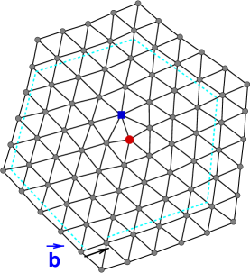
Figure 27: Example of a dislocation showing the breaking of the translational holonomy measured by the Burgers vector $\vec{b}$.

• Dislocation: represents the breaking of the translational holonomy. A path that would naturally close in a perfect lattice fails to close by a vector ${\vec{b}}$, the Burgers vector, as illustrated in Fig.27. In a flat monolayer, the energy is

  $$E=\frac{K_{0}{\vec{b}}^{2}}{8\pi}\ln(\frac{R}{a})\ ,$$ (47)

  where $K_{0}$ is the Young Modulus. It diverges logarithmically with system size.

• Disclination: represents the breaking of the rotational holonomy. The bond angle around the point defect is a multiple of the natural bond angle in the ground state ($\frac{\pi}{3}$ in a triangular lattice), as illustrated in Fig.28 for a $+$ and $-$ disclination. The energy for a disclination in a flat monolayer is given by

  $$E=\frac{K_{0}s^{2}}{32\pi}R^{2}\ .$$ (48)

  Note the quadratic divergence of the energy with system size $R$.

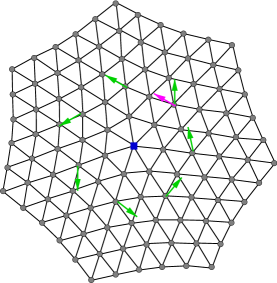
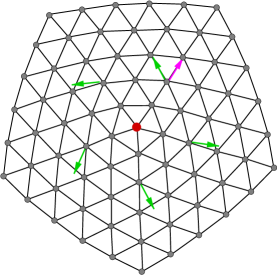
Figure 28: Example of a minus disclination (left figure) and a plus disclination (right figure). The orientational holonomy is broken by $\pm\frac{\pi}{3}$ respectively.

Inspection of Fig.27 shows that a dislocation may be regarded as a tightly bound +,- disclination pair.

6.1.1 Topological Defects in fluctuating geometries

The problem of understanding topological defects when the geometry is allowed to fluctuate was addressed in [100] (see [101] for a review). The important new feature is that the energy of a disclination defect may be lowered considerably if the membrane buckles out-of-the-plane. That is, the membrane trades elastic energy for bending rigidity. The energy for a buckled free disclination is given by

$$E=f(\kappa,K_{0},q_{i})\ln(\frac{R}{a})\ ,$$ (49)

where $f$ is some complicated function that may be evaluated numerically for given values of the parameters. It depends explicitly on $q_{i}$, which implies that the energies for positive and negative disclinations may be different, unlike the situation in flat space. The extraordinary reduction in energy from $R^{2}$ to $\ln R$ is possible because the buckled membrane creates positive Gaussian curvature for the plus-disclination and negative curvature for the negative-disclination. This is a very important physical feature of defects on curved surfaces. The defects attempt to screen out like-sign curvature, and analogously, like-sign defects may force the surface to create like-sign curvature in order to minimize the energy.

The reduction in energy for a dislocation defect is even more remarkable, since the energy of a dislocation becomes a constant, independent of the system size, provided the system is larger than a critical radius $R_{c}$. Again, by allowing the possibility of out-of-plane buckling, a spectacular reduction in energy is achieved (from $R^{2}$ to $\ln R$).

The study of other topological defects, e.g. vacancies, interstitials, and grain boundaries, may be carried out along the same lines. Since we are not going to make use of it, we refer the reader to the excellent review in [101].

6.1.2 Melting and the hexatic phase

The celebrated Kosterlitz-Thouless argument shows that defects will necessarily drive a 2D crystal to melt. The entropy of a dislocation grows logarithmically with the system size, so for sufficiently high temperature, entropy will dominate over the dislocation energy (Eq.(47)) and the crystal will necessarily melt. If the same Kosterlitz-Thouless is applied now to a tethered membrane, the entropy is still growing logarithmically with the system size, while the energy becomes independent of the system size, as explained in the previous subsection, so any finite temperature drive the crystal to melt, and the low temperature phase of a tethered membrane will necessarily be a fluid phase, either hexatic if the KTNHY melting can be applied, or a conventional fluid if a first order transition takes place, or even some other more perverse possibility. This problem has also been investigated in numerical simulations [102], which provide some concrete evidence in favor of the KTNHY scenario, although the issue is far from being settled.

It is apparent from these arguments that a hexatic membrane is a very interesting and possibly experimentally relevant membrane to understand.

6.2 The Hexatic membrane

The hexatic membrane is a fluid membrane that, in contrast to a conventional fluid, preserves the orientational order of the original lattice (six-fold (hexatic) for a triangular lattice). The mathematical description of a fluid membrane is very different from those with crystalline order. Since the description cannot depend on internal degrees of freedom, the free energy must be invariant under reparametrizations of the internal coordinates (that is, should depend only on geometrical quantities, or in more mathematical terminology, must be diffeomorphism invariant). The corresponding free energy was proposed by Helfrich [103] and it is given by

$$\frac{{\cal H}_{H}}{T}=\mu\int\sqrt{g}+\frac{\kappa}{2}\int d{\bf x}\sqrt{g}{\vec{H}}^{2}\ ,$$ (50)

where $\mu$ is the bare string tension, $\kappa$ the bending rigidity, $g$ is the determinant of the metric of the surface

$$g_{\mu\nu}({\bf x})=\partial_{\mu}{\vec{r}}({\bf x})\partial_{\nu}{\vec{r}}({\bf x})$$ (51)

and ${\vec{H}}$ is the mean Gaussian curvature of the surface. For a good description of the differential geometry relevant to the study of membranes we refer to [104] A hexatic membrane has an additional degree of freedom, the bond angle, which is introduced as a field on the surface $\theta$. The hexatic free energy [105] is obtained from adjoining to the fluid case of Eq.(50), the additional energy of the bond angle

$${\cal H}_{hex}/T=\frac{K_{A}}{2}\int d{\bf x}\sqrt{g}g^{\mu\nu}(\partial_{\mu}\theta+\Omega_{sing}-\Omega^{L}_{\mu})(\partial_{\nu}\theta+\Omega_{sing}-\Omega^{L}_{\nu})$$ (52)

where $K_{A}$ is called the hexatic stiffness, and $\Omega_{\mu}$ is the connection two form of the metric, which may be related to the Gaussian curvature of the surface by

$$K({\bf x})=\frac{1}{\sqrt{g}}\epsilon^{\mu\nu}\partial_{\mu}\Omega_{\nu}$$ (53)

and $\Omega_{sing}$ is similarly related to the topological defect density

$$s({\bf x}) = \frac{1}{\sqrt{g}}\epsilon^{\mu\nu}\partial_{\mu}\Omega_{sing\nu}$$

$$s({\bf x}) = \frac{\pi}{3}\frac{1}{\sqrt{g}}\sum_{i=1}^{N}q_{i}\delta({\bf x},{\bf x}_{i})\ .$$ (54)

From general theorems on differential geometry one has the relation

$$\int\sqrt{g}s({\bf x})=4\pi\rightarrow\sum_{i=1}^{i}q_{i}=2\chi\ ,$$ (55)

where $\chi$ is the Euler characteristic of the surface.

Therefore the total free energy for the hexatic membrane is given by

$${\cal H}/T = \mu\int\sqrt{g}+\frac{\kappa}{2}\int d{\bf x}\sqrt{g}{\vec{H}}^{2}+$$

$$+ \frac{K_{A}}{2}\int d{\bf x}\sqrt{g}g^{\mu\nu}(\partial_{\mu}\theta+\Omega_{sing}-\Omega^{L}_{\mu})(\partial_{\nu}\theta+\Omega_{sing}-\Omega^{L}_{\nu})\ .$$

The partition function is therefore

$${\cal Z}(\beta) = \sum_{N_{+},N_{-}}\frac{\delta_{N_{+}-N_{-},2\chi}}{N_{+}!N_{-}!}y^{N_{+}+N_{-}}\times$$

$$\int D[{\vec{r}}]D[{\theta}]\int\prod_{\mu=1}^{N_{+}}d{\bf x}^{+}_{\mu}\sqrt{g}\prod_{\nu=1}^{N_{-}}d{\bf x}_{\nu}^{-}\sqrt{g}e^{-{\cal H}({\vec{r}}({\bf x}),\theta({\bf x}))/T}\ ,$$

where $y$ is the fugacity of the disclination density. The partition function includes a discrete sum over allowed topological defects, those satisfying the topological constraint Eq.(55), and a path integral over embeddings ${\vec{r}}$ and bond angles $\theta$. The previous model remains quite intractable since the sum over defects interaction is very difficult to deal with.

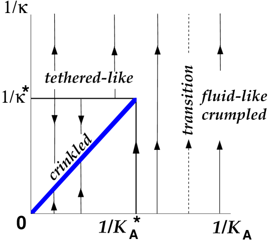
Figure 29: Phase diagram according to [106]. The hexatic membrane interpolates between a crystalline membrane and a fluid one. For small rigidity and large hexatic stiffness the RG flows towards a fluid crumpled phase. For small hexatic stiffness and large $\kappa$ it flows towards a tethered like phase, whereas for both large $\kappa$ and $K_{A}$ the flow is to the crinkled phases described by the non-trivial FP of Eq.(6.2).

Fortunately, the limit of very low fugacity $y\rightarrow 0$ is analytically tractable as was shown in the beautiful paper [107]. The RG functions can be computed within a combined large $d$ and large bending rigidity expansion. The $\beta$ functions in that limit is given by

$$\beta(\alpha) = \frac{1}{4\pi K_{A}}\left(-D\alpha^{2}+\frac{3}{4}\alpha^{3}+{\cal O}(1/K_{A}^{2})\right)\ ,$$

$$\beta(K_{A}) = 0$$ (58)

where $\alpha=1/\kappa$. The physics of hexatic membranes in the limit of very low fugacity is very rich and show a line of fixed points parametrized by the hexatic stiffness $K_{A}$. The normal-normal correlation function, for example, reads [107]

$$\langle{\vec{n}}({\bf r}){\vec{n}}({\bf 0})\rangle\sim|{\bf x}|^{-\eta}\ ,$$ (59)

with $\eta=\frac{2}{3\pi}d(d-2)\frac{k_{B}T}{K_{A}}$. The FPs of Eq.(6.2) describe a new crinkled phase, more rigid than a crumpled phase but more crumpled than a flat one. The Hausdorff dimension at the crinkled phase is given by [107]

$$d_{H}=2+\frac{d(d-2)}{3\pi}\frac{k_{B}T}{K_{A}}\ .$$ (60)

From the RG point of view, the properties of these crinkled phases are really interesting, since they involve a line of Fixed Points which are inequivalent in the sense that the associated critical exponents depend continuously on $K_{A}$, a situation reminiscent of the $XY$-model. In [106] the phase diagram is discussed, and the authors propose the scenario depicted in Fig.29. How these scenarios are modified when the fugacity is considered is not well established and we refer the reader to the original papers [108, 109, 106].

The shape fluctuations of hexatic vesicles, for large defect core energies, have also been investigated [110, 111].

7 The Fluid Phase

The study of fluid membranes is a broad subject, currently under intense experimental and theoretical work. The Hamiltonian is given by

$${\cal H}/T=\mu\int\sqrt{g}+\frac{\kappa}{2}\int d{\bf x}\sqrt{g}{\vec{H}}^{2}+\frac{\hat{\kappa}}{2}\int\sqrt{g}K\ ,$$ (61)

This corresponds to the Helfrich hamiltonian together with a term that allows for topology changing interactions. For fixed topology it is well-known [112, 113, 114, 115] that the one loop beta function for the inverse-bending rigidity has a fixed point only at $\kappa=0$, which corresponds to the bending rigidity being irrelevant at large length scales. The RG flow of the bending rigidity is given by

$$\kappa(l)=\kappa_{o}-\frac{3T}{4\pi}{\rm ln}(l/a)\ ,$$ (62)

where a is a microscopic cutoff length. The fluid membrane is therefore crumpled, for arbitrary microscopic bending rigidity $\kappa_{0}$, at length scales beyond a persistence length which grows exponentially with $\kappa_{0}$. For a fluid membrane out-of-plane fluctuations cost no elastic energy (the membrane flows internally to accommodate the deformation) and the bending rigidity is therefore softened by thermal undulations at all length scales, rather than stiffening at long length scales as in the crystalline membrane.

So far we have assumed an infinite membrane, which is not always a realistic assumption. A thickness may be taken into account via a spontaneous extrinsic curvature ${\vec{H}}_{0}$. The model described by Eq. 61 gets replaced then by

$${\cal H}/T=\mu\int\sqrt{g}+\frac{\kappa}{2}\int d{\bf x}\sqrt{g}({\vec{H}-\vec{H}_{0}})^{2}+\frac{\hat{\kappa}}{2}\int\sqrt{g}K\ .$$ (63)

Further effects of a finite membrane size for spherical topology have been discussed in [116, 117, 118]. The phase diagram of fluid membranes when topology change is allowed is fascinating and not completely understood. A complete description of these phases goes beyond the scope of this review – we refer the reader to [48, 49, 22, 25] and references therein.

8 Conclusions

In this review we have described the distinct universality classes of membranes with particular emphasis on crystalline membranes. In each case we discussed and summarized the key models describing the interactions of the relevant large distance degrees of freedom (at the micron scale). The body of the review emphasizes qualitative and descriptive aspects of the physics with technical details presented in extensive appendices. We hope that the concreteness of these calculations gives a complete picture of how to extract relevant physical information from these membrane models.

We have also shown that the phase diagram of the phantom crystalline membrane class is theoretically very well understood both by analytical and numerical treatments. To complete the picture it would be extremely valuable to find experimental realizations for this particular system. An exciting possibility is a system of cross-linked DNA chains together with restriction enzymes that catalyze cutting and rejoining [119]. The difficult chemistry involved in these experiments is not yet under control, but we hope that these technical problems will be overcome in the near future.

There are several experimental realizations of self-avoiding polymerized membranes discussed in the text. The experimental results compare very well with the theoretical estimates from numerical simulations. As a future theoretical challenge, analytical tools need to be sharpened since they fail to provide a clear and unified picture of the phase diagram. On the experimental side, there are promising experimental realizations of tethered membranes which will allow more precise results than those presently available. Among them there is the possibility of very well controlled synthesis of DNA networks to form physical realizations of tethered membranes.

The case of anisotropic polymerized membranes has also been described in some detail. The phase diagram contains a new tubular phase which may be realized in nature. There is some controversy about the precise phase diagram of the model, but definite predictions for the critical exponents and other quantities exist. Anisotropic membranes are also experimentally relevant. They may be created in the laboratory by polymerizing a fluid membrane in the presence of an external electric field.

Probably the most challenging problem, both theoretically and experimental, is a complete study of the role of defects in polymerized membranes. There are a large number of unanswered questions, which include the existence of hexatic phases, the properties of defects on curved surfaces and its relevance to the possible existence of more complex phases. This problem is now under intense experimental investigation. In this context, let us mention very recent experiments on Langmuir films in a presumed hexatic phase [120]. The coalescence of air bubbles with the film exhibit several puzzling features which are strongly related to the curvature of the bubble.

Crystalline membranes also provide important insight into the fluid case, since any crystalline membrane eventually becomes fluid at high temperature. The physics of fluid membranes is a complex and fascinating subject in itself which goes beyond the scope of this review. We highlighted some relevant experimental realizations and gave a quick overview of the existing theoretical models. Due to its relevance in many physical and biological systems and its potential applications in material science, the experimental and theoretical understanding of fluid membranes is, and will continue to be, one of the most active areas in soft condensed matter physics.

We have not been able in this review, simply for lack of time, to address the important topic of the role of disorder. We hope to cover this in a separate article.

We hope that this review will be useful for physicists trying to get a thorough understanding of the fascinating field of membranes. We think it is a subject with significant prospects for new and exciting developments.

Note: The interested reader may also find additional material in a forthcoming review by Wiese [121], of which we have seen only the table of contents.

Acknowledgements

This work was supported by the U.S. Department of Energy under contract No. DE-FG02-85ER40237. We would like to thank Dan Branton and Cyrus Safinya for providing us images from their laboratories and Paula Herrera-Siklódy for assistance with the figures. MJB would like to thank Riccardo Capovilla, Chris Stephens, Denjoe O’Connor and the other organizers of RG2000 for the opportunity to attend a wonderful meeting in Taxco, Mexico.

Appendix A Useful integrals in dimensional regularization

In performing the $\varepsilon$-expansion, we will be considering integrals of the form

$$I_{\alpha_{1},\cdots,\alpha_{n}}(a,b)({\vec{p}})=\int d^{D}\hat{q}\frac{q_{\alpha_{1}}\cdots q_{\alpha_{n}}}{(\vec{p}+\vec{q})^{2a}\vec{q}^{2b}}\ ,$$ (64)

These integrals may be computed exactly for general $D,a,b$ and $\alpha=1,\cdots,N$. The result will be published elsewhere. We will content ourselves by quoting what we need, the poles in $\varepsilon$, for the integrals that appear in the diagrammatic calculations. We just quote the results

$$I_{\alpha_{1}\alpha_{2}}(2,2)=-\frac{1}{8\pi^{2}p^{4}}p_{\alpha_{1}}p_{\alpha_{2}}\frac{1}{\varepsilon}$$ (65)

$$I_{\alpha_{1}\alpha_{2}\alpha_{3}}(2,2)=\frac{1}{8\pi^{2}p^{4}}p_{\alpha_{1}}p_{\alpha_{2}}p_{\alpha_{3}}\frac{1}{\varepsilon}$$ (66)

$$I_{\alpha_{1}\alpha_{2}\alpha_{3}\alpha_{4}}(2,2)=-\frac{1}{8\pi^{2}p^{4}}\left(p_{\alpha_{1}}p_{\alpha_{2}}p_{\alpha_{3}}p_{\alpha_{4}}-\right.$$

$$\left.\frac{p^{4}}{24}(\delta_{\alpha_{1}\alpha_{2}}\delta_{\alpha_{3}\alpha_{4}}+\delta_{\alpha_{1}\alpha_{3}}\delta_{\alpha_{2}\alpha_{4}}+\delta_{\alpha_{1}\alpha_{4}}\delta_{\alpha_{2}\alpha_{3}})\right)\frac{1}{\varepsilon}$$ (67)

$$I_{\alpha_{1}\alpha_{2}\alpha_{3}}(2,1) = -\frac{1}{8\pi^{2}p^{2}}(\frac{p^{2}}{6}(p_{\alpha_{1}}\delta_{\alpha_{2}\alpha_{3}}+p_{\alpha_{2}}\delta_{\alpha_{1}\alpha_{3}}+p_{\alpha_{3}}\delta_{\alpha_{2}\alpha_{1}})$$ (68)

$$-p_{\alpha_{1}}p_{\alpha_{2}}p_{\alpha_{3}})\frac{1}{\varepsilon}$$

Appendix B Some practical identities for RG quantities

The beta functions defined in Eq. 3 may be re-expressed as

$$\left(\begin{array}[]{cc}\beta_{u}(u_{R},v_{R})\\ \beta_{v}(u_{R},v_{R})\end{array}\right)=-\varepsilon\left(\begin{array}[]{cc}\frac{\partial\ln u}{\partial u_{R}}&\frac{\partial\ln u}{\partial v_{R}}\\ \frac{\partial\ln v}{\partial u_{R}}&\frac{\partial\ln v}{\partial v_{R}}\end{array}\right)^{-1}\left(\begin{array}[]{cc}1\\ 1\end{array}\right)$$ (69)

The previous expression may be further simplified noticing

$$A=\left(\begin{array}[]{cc}\frac{\partial\ln u}{\partial u_{R}}&\frac{\partial\ln u}{\partial v_{R}}\\ \frac{\partial\ln v}{\partial u_{R}}&\frac{\partial\ln v}{\partial v_{R}}\end{array}\right)=\left(\begin{array}[]{cc}\frac{1}{u_{R}}&0\\ 0&\frac{1}{v_{R}}\end{array}\right)+D\ ,$$ (70)

so that

$$A^{-1} = \left(1+\left(\begin{array}[]{cc}u_{R}&0\\ 0&v_{R}\end{array}\right)D\right)^{-1}\left(\begin{array}[]{cc}u_{R}&0\\ 0&v_{R}\end{array}\right)$$ (75)

$$= \left(\begin{array}[]{cc}u_{R}&0\\ 0&v_{R}\end{array}\right)-\left(\begin{array}[]{cc}u_{R}&0\\ 0&v_{R}\end{array}\right)D\left(\begin{array}[]{cc}u_{R}&0\\ 0&v_{R}\end{array}\right)+\cdots$$ (82)

where the last result follows from Taylor-expanding. These formulas easily allow to compute the corresponding $\beta$-functions. If

$$u = M^{\varepsilon}\left[u_{R}+\frac{1}{\varepsilon}(a_{11}u^{2}_{R}+a_{12}u_{R}v_{R}+a_{13}v^{2}_{R})\right]$$ (83)

$$v = M^{\varepsilon}\left[v_{R}+\frac{1}{\varepsilon}(a_{21}u^{2}_{R}+a_{22}u_{R}v_{R}+a_{23}v^{2}_{R})\right]\ ,$$

from Eq. 75 and Eq. 69 we easily derive the leading two orders in the couplings

$$\beta_{u}(u_{R},v_{R}) = -\varepsilon u_{R}+a_{11}u^{2}_{R}+a_{12}u_{R}v_{R}+a_{13}v^{2}_{R}$$ (84)

$$\beta_{v}(u_{R},v_{R}) = -\varepsilon v_{R}+a_{21}u^{2}_{R}+a_{22}u_{R}v_{R}+a_{23}v^{2}_{R}\ .$$

The formula for $\gamma$ in Eq. 3 may also be given a more practical expression. It is given by

$$\gamma=(\beta_{u}\frac{\partial}{\partial u_{R}}+\beta_{v}\frac{\partial}{\partial v_{R}})\ln Z_{\phi}\ ,$$ (85)

Those are the formulas we need in the calculations we present in this review.

Appendix C Discretized Model for tethered membranes

In this appendix we present appropriate discretized models for numerical simulation of tethered membranes. The surface is discretized by a triangular lattice defined by its vertices $\{{\vec{r}}\}_{a=1,\cdots}$, with a corresponding discretized version of the Landau elastic term Eq. 20 given by [100]

$$F_{s}=\frac{\beta}{2}\sum_{\langle ab\rangle}(|{\vec{r}}_{a}-{\vec{r}}_{b}|-1)^{2}\ ,$$ (86)

where $\langle a,b\rangle$ are nearest-neighbor vertices. If we write ${\vec{r}}_{a}={\bf x}_{a}+{\bf u}_{a}$ with ${\bf x}_{a}$ defining the vertices of a perfectly regular triangular lattice and ${\bf u}$ the small perturbations around it, one gets

$$|{\vec{r}}_{a}-{\vec{r}}_{b}|=1+u_{\alpha\beta}x^{\alpha}x^{\beta}+\cdots\ ,$$ (87)

with $u_{\alpha\beta}$ being a discretized strain tensor and we we have neglected higher order terms. Plugging the previous expression into Eq. 86 and passing from the discrete to the continuum language we obtain

$$F_{s}=\frac{\sqrt{3}}{8}\beta\int d^{2}{\bf x}(2u^{2}_{\alpha\beta}+u^{2}_{\alpha\alpha})$$ (88)

which is the elastic part of the free energy Eq. 20 with $\lambda=\mu=\frac{\sqrt{3}}{4}\beta$.

The bending rigidity term is written in the continuum as

$$S_{ext}=\int d^{2}{\bf x}\sqrt{g}K^{\mu}_{\alpha\beta}K_{\mu}^{\alpha\beta}=\int d^{2}{\bf u}\sqrt{g}g^{\alpha\beta}\nabla_{\alpha}{\vec{n}}\nabla_{\beta}{\vec{n}}$$ (89)

where ${\vec{n}}$ is the normal to the surface and $\nabla$ is the covariant derivative (see [122] for a detailed description of these geometrical quantities). We discretize the normals form the the previous equation by

$$\int d^{2}{\bf u}\sqrt{g}g^{\alpha\beta}\nabla_{\alpha}{\vec{n}}\nabla_{\beta}{\vec{n}}\rightarrow\sum_{\langle ab\rangle}({\vec{n}}_{a}-{\vec{n}}_{b})^{2}=2\sum_{\langle ab\rangle}(1-{\vec{n}}_{a}{\vec{n}}_{b})$$ (90)

The two terms Eq. 86 and Eq. 90 provide a suitable discretized model for a tethered membranes. However, in actual simulations, the even more simplified discretization

$$F=\sum_{\langle a,b\rangle}({\vec{r}}_{a}-{\vec{r}}_{b})^{2}+\kappa\sum_{\langle i,j\rangle}(1-{\vec{n}}_{i}{\vec{n}}_{j})$$ (91)

is preferred since it is simpler and describes the same universality class (see [38] for a discussion). Anisotropy may be introduced in this model by ascribing distinct bending rigidities to bending across links in different intrinsic directions [92].

Self-avoidance can be introduced in this model by imposing that the triangles that define the discretized surface cannot self-intersect. There are other possible discretizations of self-avoidance that we discus in sect. 4.2.

In order to numerically simulate the model Eq. 91 different algorithms have been used. A detailed comparison of the performance of each algorithm may be found in [123].

Appendix D The crumpling Transition

The Free energy is given by Eq. 13

$$F({\vec{r}})=\int d^{D}{\bf x}\left[\frac{1}{2}(\partial_{\alpha}^{2}{\vec{r}})^{2}+u(\partial_{\alpha}{\vec{r}}\partial_{\beta}{\vec{r}}-\frac{\delta_{\alpha\beta}}{D}(\partial_{\alpha\vec{r}})^{2})^{2}+v(\partial_{\alpha}{\vec{r}}\partial^{\alpha}{\vec{r}})^{2}\right]\ ,$$ (92)

where the dependence on $\kappa$ is trivially scaled out. The Feynman rules for the model are given in Fig.30.

Figure 30: Feynman rules for the model at the crumpling transition

We need three renormalized constants, namely $Z$, $Z_{u}$ and $Z_{v}$ in order to renormalize the theory. We define the renormalized quantities by

$${\vec{r}} = Z^{-1/2}{\vec{r}}$$ (93)

$$u_{R}=M^{-\varepsilon}Z^{2}Z_{u}^{-1}u \ , v_{R}=M^{-\varepsilon}Z^{2}Z_{v}^{-1}v\ .$$

Then Eq. 92 becomes

$$F({\vec{r}}) = \int d^{D}{\bf x}\left[\frac{Z}{2}(\partial_{\alpha}^{2}{\vec{r}_{R}})^{2}+M^{\varepsilon}Z_{u}u(\partial_{\alpha}{\vec{r}_{R}}\partial_{\beta}{\vec{r}_{R}}-\frac{\delta_{\alpha\beta}}{D}(\partial_{\alpha}\vec{r}_{R})^{2})^{2}\right.+$$ (94)

$$+ \left.M^{\varepsilon}Z_{v}v(\partial_{\alpha}{\vec{r}_{R}}\partial^{\alpha}{\vec{r}_{R}})^{2}\right]\ ,$$

In order to compute the renormalized couplings, one must compute all relevant diagrams at one loop. Those are depicted in fig. 31. Within dimensional regularization, diagrams (1a) and (1b) are zero, which in turns imply that the renormalized constant is $Z=1$ at leading order in $\varepsilon$, similarly as in linear $\sigma$ models.

Figure 31: Diagrams to consider at one loop

Using the integrals in dimensional regularization (see Sect. A) Diagram (2a) gives the result

$$\frac{d}{8\pi^{2}}\frac{1}{\varepsilon}\delta^{i_{1}i_{2}}\delta^{j_{1}j_{2}}\left\{\frac{u^{2}}{24}(\vec{p}_{1}\cdot\vec{p}_{3}\vec{p}_{2}\cdot\vec{p}_{4}+\vec{p}_{1}\cdot\vec{p}_{4}\vec{p}_{2}\cdot\vec{p}_{3})+(v^{2}-\frac{u^{2}}{48})\vec{p}_{1}\cdot\vec{p}_{2}\vec{p}_{3}\cdot\vec{p}_{4}\right\}$$ (95)

And diagram (2b) and (2c) may be computed at once, since the result of (2c) is just (2b) after interchanging $\vec{p}_{3}\leftrightarrow\vec{p}_{4}$, so the total result (2a)+(2b) is

$$\frac{1}{16\pi^{2}}\frac{1}{\varepsilon}\delta^{i_{1}i_{2}}\delta^{j_{1}j_{2}}\left\{(\frac{61}{96}u^{2}+\frac{7}{12}uv+\frac{v^{2}}{6})(\vec{p}_{1}\cdot\vec{p}_{3}\vec{p}_{2}\cdot\vec{p}_{4}\right.+\vec{p}_{1}\cdot\vec{p}_{4}\vec{p}_{2}\cdot\vec{p}_{3})$$

$$\left.+(\frac{v^{2}}{6}+\frac{uv}{12}+\frac{u^{2}}{96})\vec{p}_{1}\cdot\vec{p}_{2}\vec{p}_{3}\cdot\vec{p}_{4}\right\}$$ (96)

And the result for (2d) and (2e) is just identical, so the total result (2d)+(2e) is

$$\frac{1}{16\pi^{2}}\frac{1}{\varepsilon}\delta^{i_{1}i_{2}}\delta^{j_{1}j_{2}}\left\{(\frac{u^{2}}{24}+\frac{1}{6}uv)(\vec{p}_{1}\cdot\vec{p}_{3}\vec{p}_{2}\cdot\vec{p}_{4}\right.+\vec{p}_{1}\cdot\vec{p}_{4}\vec{p}_{2}\cdot\vec{p}_{3})$$

$$\left.+(v^{2}+\frac{13}{6}uv-\frac{u^{2}}{48})\vec{p}_{1}\cdot\vec{p}_{2}\vec{p}_{3}\cdot\vec{p}_{4}\right\}$$ (97)

Adding up all these contributions taking into account the different combinatorial factors (4 the first contribution, 8 the last two ones) and recalling $Z=1$, we get

$$u = M^{\varepsilon}\left[u_{R}+\frac{1}{\varepsilon}\frac{1}{8\pi^{2}}\left((\frac{d}{3}+\frac{65}{12})u^{2}_{R}+6u_{R}v_{R}+\frac{4}{3}v^{2}_{r}\right)\right]$$

$$v = M^{\varepsilon}\left[v_{R}+\frac{1}{\varepsilon}\frac{1}{8\pi^{2}}\left(\frac{21}{16}u_{R}+\frac{21}{2}u_{R}v_{R}+(4d+5)v^{2}_{R}\right)\right]\ .$$ (98)

The resultant $\beta$-functions are then readily obtained by applying Eq.(84).

Appendix E The Flat Phase

The free energy is given in Eq. 20,and it is given by

$$F({\bf u},h)=\int d^{D}{\bf x}\left[\frac{\hat{\kappa}}{2}(\partial_{\alpha}\partial_{\beta}h)^{2}+\mu u_{\alpha\beta}u^{\alpha\beta}+\frac{\lambda}{2}(u^{\alpha}_{\alpha})^{2}\right]\,.$$ (99)

The Feynman rules are shown in fig. 32, it is apparent that the in-plane phonons couple different from the out-of-plane, which play the role of Goldstone bosons.

Figure 32: Feynman rules for the model in the flat phase

We apply standard field theory techniques to obtain the RG-quantities. Using the Ward identities, the theory can be renormalized using only three renormalization constants $Z$, $Z_{\mu}$ and $Z_{\lambda}$, corresponding to the wave function and the two coupling renormalizations. Renormalized quantities read

$$h_{R}=Z^{-1/2}h \ , {\bf u}=Z^{-1}{\bf u}$$ (100)

$$\mu_{R}=M^{-\varepsilon}Z^{2}Z_{\mu}^{-1}\mu \ , \lambda_{R}=M^{-\varepsilon}Z^{2}Z_{\lambda}^{-1}\lambda\ ,$$

Then Eq. 99 becomes

$$F({\bf u},h)=\int d^{D}{\bf x}\left[Z(\partial_{\alpha}\partial_{\beta}h_{R})^{2}+2M^{\varepsilon}Z_{\mu}\mu_{R}u_{R\alpha\beta}u^{\alpha\beta}_{R}+M^{\varepsilon}Z_{\lambda}\lambda(u^{\alpha}_{R\alpha})^{2}\right]\,.$$ (101)

We now compute the renormalized quantities from the leading divergences appearing in the Feynman diagrams. The diagrams to consider are given in Fig.33. These can be computed using the integrals given in Sect.A.

Figure 33: Diagrams to consider at one loop

The result of diagram (1a) is given by

$$\frac{1}{\varepsilon}\frac{d_{c}}{6\pi^{2}}\left[\mu^{2}(\delta_{\alpha\beta}-\frac{p_{\alpha}p_{\beta}}{p^{2}})+3(\mu^{2}+2\mu\lambda+2\lambda^{2})\frac{p_{\alpha}p_{\beta}}{p^{2}}\right]p^{2}\ .$$ (102)

Diagrams (2b) and (2c) are identically zero, so (2a) is the only additional diagram to be computed. The result is

$$-\frac{1}{\varepsilon}\frac{\delta^{ij}}{8\pi^{2}}\frac{\mu(\mu+\lambda)}{2\mu+\lambda}10(p^{2})^{2}$$ (103)

from Eq. 103 and the definitions in Eq. 100

$$Z=1-\frac{1}{\varepsilon}\frac{10}{8\pi^{2}}\frac{\mu_{R}(\mu_{R}+\lambda_{R})}{2\mu_{R}+\lambda_{R}}\ .$$ (104)

Using the previous result in the diagrams (1a) whose result is in Eq. 102 we obtain

$$Z_{\mu} = 1+\frac{1}{\varepsilon}\frac{d_{c}}{24\pi^{2}}\mu_{R}$$ (105)

$$Z_{\lambda} = 1+\frac{1}{\varepsilon}\frac{d_{c}}{24\pi^{2}}(\mu^{2}_{R}+6\mu_{R}\lambda_{R}+6\lambda_{R}^{2})/\lambda_{R}$$

and we deduce the renormalized couplings

$$\mu = M^{\varepsilon}\left[\mu_{R}+\frac{1}{\varepsilon}\left(\frac{10}{4\pi^{2}}\frac{(\mu_{R}+\lambda_{R})}{2\mu_{R}+\lambda_{R}}+\frac{d_{c}}{24\pi^{2}}\right)\mu^{2}_{R}\right]$$ (106)

$$\lambda = M^{\varepsilon}\left[\lambda_{R}+\frac{1}{\varepsilon}\left(\frac{10}{4\pi^{2}}\frac{(\mu_{R}+\lambda_{R})}{2\mu_{R}+\lambda_{R}}\mu_{R}\lambda_{R}+\frac{d_{c}}{24\pi^{2}}(\mu^{2}_{R}+6\mu_{R}\lambda_{R}+6\lambda^{2}_{R})\right)\right]$$

from which the $\beta$-functions trivially follow with the aid of Eq.(84).

Appendix F The Self-avoiding phase

The model has been introduced in Eq. 31 and is given by

$$F({\vec{r}})=\frac{1}{2}\int d^{D}{\bf x}(\partial_{\alpha}{\vec{r}}({\bf x}))^{2}+\frac{b}{2}\int d^{D}{\bf x}\,d^{D}{\bf y}\delta^{d}({\vec{r}}({\bf x})-{\vec{r}}({\bf y}))\ ,$$ (107)

We follow the usual strategy of defining the renormalized quantities by

$${\vec{r}} = Z^{1/2}{\vec{r}}_{R}$$ (108)

$$b = M^{\varepsilon}Z_{b}Z^{d/2}b_{R}\ ,$$

and the renormalized Free energy by

$$F({\vec{r}})=\frac{Z}{2}\int d^{D}{\bf x}(\partial_{\alpha}{\vec{r}}_{R}({\bf x}))^{2}+M^{\varepsilon}Z_{b}\frac{b_{R}}{2}\int d^{D}{\bf x}\,d^{D}{\bf y}\delta^{d}({\vec{r}}_{R}({\bf x})-{\vec{r}}_{R}({\bf y}))\ .$$ (109)

The $\delta$-function being non-local adds some technical difficulties to the calculation of the renormalized constants $Z$ and $Z_{b}$. There are different approaches available but we will follow the MOPE (Multilocal-Operator-Product-Expansion), which we will just explain in a very simplified version. A rigorous description of the method may be found in the literature.

The idea is to expand the $\delta$-function term in Eq. 109

$$e^{-F({\vec{r}})}=e^{-\frac{Z}{2}\int d^{D}{\bf x}(\partial_{\alpha}{\vec{r}}_{R}({\bf x}))^{2}}\times\sum_{n=0}^{\infty}\left(-M^{\varepsilon}Z_{b}\frac{b_{R}}{2}\int d^{D}{\bf x}\,d^{D}{\bf y}\delta^{d}({\vec{r}}_{R}({\bf x})-{\vec{r}}_{R}({\bf y}))\right)^{n}\ ,$$ (110)

with this trick, the delta-function term may be treated as expectation values of a Gaussian free theory. This observation alone allows to isolate the poles in $\varepsilon$. We write the identity

$$e^{i{\vec{k}}({\vec{r}}({\bf x}_{1})-{\vec{r}}({\bf x}_{2}))}=:e^{i{\vec{k}}({\vec{r}}({\bf x}_{1})-{\vec{r}}({\bf x}_{2}))}:e^{k^{2}G(x_{1}-x_{2})}\ ,$$ (111)

where $G(x)$ is the two point correlator

$$-G({\bf x})=-\langle{\vec{r}}({\bf x}){\vec{r}}(0)\rangle=\frac{|{\bf x}|^{2-D}}{(2-D)S_{D}}\ ,$$ (112)

with $S_{D}$ being the volume of the $D$-dimensional sphere. The symbol $::$ stands for normal ordering. A normal ordered operator is non-singular at short-distances, so it may be Taylor-expanded

$$e^{i{\vec{k}}({\vec{r}}({\bf x}_{1})-{\vec{r}}({\bf x}_{2}))} = (1+i({\bf x_{1}-x_{2}})^{\alpha}({\vec{k}}\partial_{\alpha}{\vec{r}})$$

$$-\frac{1}{2}({\bf x_{1}-x_{2}})^{\alpha}({\bf x_{1}-x_{2}})^{\beta}({\vec{k}}\partial_{\alpha}{\vec{r}})({\vec{k}}\partial_{\beta}{\vec{r}})+\cdots)e^{k^{2}G(x_{1}-x_{2})}\ .$$

To isolate the poles in $\varepsilon$ we do not need to consider higher order terms as it will become clear. If we now integrate over ${\vec{k}}$, we get

$$\delta^{d}({\vec{r}}({\bf x}_{1})-\vec{r}({\bf x}_{2})) = \frac{1}{(4\pi)^{d/2}(-G({\bf x}_{1}-{\bf x}_{2}))^{d/2}}1$$

$$-\frac{1}{4}\frac{({\bf x}_{1}-{\bf x}_{2})^{\alpha}({\bf x}_{1}-{\bf x}_{2})^{\beta}}{(4\pi)^{d/2}(-G({\bf x}_{1}-{\bf x}_{2}))^{d/2+1}}\partial_{\beta}{\vec{r}}({\bf x})\partial_{\alpha}{\vec{r}}({\bf x})+\cdots$$

$$\equiv C^{1}({\bf x}_{1}-{\bf x}_{2})1+C^{\alpha\beta}({\bf x}_{1}-{\bf x}_{2})\partial_{\beta}{\vec{r}}({\bf x})\partial_{\alpha}{\vec{r}}({\bf x})+\cdots$$

where we omit higher dimensional operators in ${\vec{r}}$, which are irrelevant by power counting, so since the theory is renormalizable they cannot have simple poles in $\varepsilon$. Additionally, we have defined ${\bf x}=\frac{{\bf x}_{1}+{\bf x}_{2}}{2}$. One recognizes in Eq. F Wilson’s Operator product expansion, applied to the non-local delta-function operator.

Following the same technique of splitting the operator into a normal ordered part and a singular part at short-distances, it just takes a little more effort to derive the OPE for the product of two delta functions, the result is

$$\delta^{d}({\vec{r}}({\bf x}_{1})-\vec{r}({\bf y}_{1}))\delta^{d}({\vec{r}}({\bf x}_{2})-\vec{r}({\bf y}_{2}))=C({\bf x}_{1}-{\bf x}_{2},{\bf y}_{1}-{\bf y}_{2})\delta^{d}({\vec{r}}({\bf x})-\vec{r}({\bf y}))+\cdots$$ (115)

with $C({\bf x}_{1}-{\bf x}_{2},{\bf y}_{1}-{\bf y}_{2})=\frac{1}{(4\pi)^{d/2}(-G({\bf x}_{1}-{\bf x}_{2})-G({\bf y}_{1}-{\bf y}_{2}))^{d/2}}$. The terms omitted are again higher dimensional by power counting so they. The OPE Eq. F and Eq. 115 is all we need to compute the renormalization constants at lowest order in $\varepsilon$, but the calculation may be pursued to higher orders in $\varepsilon$. In order to do that, one must identify where poles in $\varepsilon$ arise. In the previous example poles in $\varepsilon$ appear whenever the internal coordinates (${\bf x}_{1}$ and ${\bf x}_{2}$ in Eq. F, ${\bf x}_{1}$,${\bf x}_{2}$,${\bf y}_{3}$ and ${\bf y}_{2}$ in Eq. 115) are pairwise made to coincide. This is diagrammatically shown in fig. 34. It is possible to show, that higher poles appear in the same way, if more $\delta$-product terms are considered.

Figure 34: Diagrammatic expansion to isolate the poles in $\varepsilon$ within the MOPE formalism at lowest non-trivial order. Solid lines represent $\delta$-function terms and dashed lines indicate that points inside are taken arbitrarily close. Higher orders contributions arise in the same way.

Let us consider the first delta-function term corresponding to $n=1$ in the sum Eq. 110. Using Eq. F we have

$$-\frac{b_{r}M^{\varepsilon}}{2}Z_{b}\int d^{D}{\bf x}\,d^{D}{\bf y}\delta^{d}({\vec{r}}_{R}({\bf x})-{\vec{r}}_{R}({\bf y}))$$

$$= -\frac{b_{r}M^{\varepsilon}}{2}Z_{b}\int d^{D}{\bf x}\,d^{D}{\bf y}(C^{1}({\bf x}-{\bf y})+C^{\alpha\beta}({\bf x}-{\bf y})\partial_{\beta}{\vec{r}}_{R}({\bf x})\partial_{\alpha}{\vec{r}}_{R}({\bf x})+\cdots$$

$$= -\frac{b_{r}M^{\varepsilon}}{2}Z_{b}\int d^{D}{\bf x}\partial_{\alpha}{\vec{r}}_{R}({\bf x})\partial^{\alpha}{\vec{r}}_{R}({\bf x})\int d^{D}{\bf y}\frac{\delta_{\alpha\beta}C^{\alpha\beta}}{D}+\cdots$$

The first term just provides a renormalization of the identity operator, which we can neglect. From

$$\int_{|{\bf y}|>1/M}d^{D}{\bf y}\frac{\delta_{\alpha\beta}C^{\alpha\beta}}{D}({\bf y})=-\frac{1}{4D}\frac{M^{-\varepsilon}}{\varepsilon}(4\pi)^{-d/2}(2-D)^{1+d/2}\left(\frac{2\pi^{D/2}}{\Gamma(D/2)}\right)^{2+d/2}\ ,$$ (117)

and we can absorb the pole by $Z$ if we define

$$Z=1+\frac{b_{R}}{\varepsilon}\frac{(4\pi)^{-d/2}}{4D}(2-D)^{1+d/2}\left(\frac{2\pi^{D/2}}{\Gamma(D/2)}\right)^{2+d/2}\ ,$$ (118)

From the short distance behavior in the sum Eq. 110 corresponding to $n=2$ we get

$$-\frac{b_{r}^{2}M^{2\varepsilon}}{8}\int d^{D}{\bf x}_{1}\,d^{D}{\bf y}_{1}d^{D}{\bf x}_{2}\,d^{D}{\bf y}_{2}\delta^{d}({\vec{r}}_{R}({\bf x}_{1})-{\vec{r}}_{R}({\bf y}_{1}))\delta^{d}({\vec{r}}_{R}({\bf x}_{1})-{\vec{r}}_{R}({\bf y}_{2}))$$

$$-\frac{b_{r}^{2}M^{2\varepsilon}}{8}\int d^{D}{\bf x}\,d^{D}{\bf y}\delta^{d}({\vec{r}}_{R}({\bf x})-{\vec{r}}_{R}({\bf y}))\int d^{D}{\bf z}\,d^{D}{\bf w}C(z,w)\ ,$$ (119)

where, in order to isolate the pole we can perform the following tricks

$$\int d^{D}{\bf z}\,d^{D}{\bf w}C(z,w)$$

$$= (4\pi)^{-d/2}S_{D}^{d/2}(2-D)^{d/2}\left(\frac{2\pi^{D/2}}{\Gamma(D/2)}\right)^{2}\int_{0}^{M^{-1}}dz\int_{0}^{M^{-1}}dw\frac{z^{D-1}w^{D-1}}{(z^{2-D}+w^{2-D})^{d/2}}$$

$$= (4\pi)^{-d/2}S_{D}^{d/2}(2-D)^{d/2}\left(\frac{2\pi^{D/2}}{\Gamma(D/2)}\right)^{2}\frac{M^{-\varepsilon}}{(2-D)^{2}}\int_{0}^{1}\int_{0}^{1}dxdy\frac{x^{\frac{D}{2-D}}y^{\frac{D}{2-D}}}{(x+y)^{-d/2}}$$

$$= (4\pi)^{-d/2}S_{D}^{d/2}(2-D)^{d/2}\left(\frac{2\pi^{D/2}}{\Gamma(D/2)}\right)^{2}\frac{M^{-\varepsilon}}{(2-D)^{2}}\int_{x^{2}+y^{2}\leq 1}dxdy\frac{x^{\frac{D}{2-D}}y^{\frac{D}{2-D}}}{(x+y)^{-d/2}}$$

$$= (4\pi)^{-d/2}S_{D}^{d/2}(2-D)^{d/2}\left(\frac{2\pi^{D/2}}{\Gamma(D/2)}\right)^{2}\frac{M^{-\varepsilon}}{(2-D)^{3}}\frac{\Gamma(\frac{D}{2-D})^{2}}{\Gamma(\frac{2D}{2-D})}\frac{1}{\varepsilon}$$

since changing the boundary of integration from a square to a circle does not affect the residue of the pole. We finally have

$$Z_{b}=1+\frac{b_{R}}{\varepsilon}\frac{1}{2}(2-D)^{-1+d/2}\frac{\Gamma(\frac{D}{2-D})^{2}}{\Gamma(\frac{2D}{2-D})}\left(\frac{2\pi^{D/2}}{\Gamma(D/2)}\right)^{2+d/2}(4\pi)^{-d/2}\ ,$$ (121)

and the $\beta$-function follows from the definitions Eq.(108) together with Eq.(118) and Eq.(84).

Appendix G The mean field solution of the anisotropic case

The free energy has been introduced in Eq. 39. Let us first show the constraints on the couplings so that the Free energy is bounded from below.

• $u_{yy}>0$: This follows trivially.

• $u^{\prime}_{\perp\perp}\equiv v_{\perp\perp}+\frac{u_{\perp\perp}}{D-1}>0$ : Define $A_{\alpha}^{i}=\partial_{\alpha}r^{i}({\bf x})$ then from Eq. 39 we get

  $$\frac{u_{\perp\perp}}{2}Tr(AA^{T})^{2}+\frac{v_{\perp\perp}}{2}(TrAA^{T})^{2}\geq(\frac{u_{\perp\perp}}{D-1}+v_{\perp\perp})/2(TrAA^{T})^{2}$$ (122)

  $$= \frac{u^{\prime}_{\perp\perp}}{2}(TrAA^{T})^{2}\ ,$$

  which implies $u_{\perp\perp}^{\prime}>0$.

• $v_{\perp y}>-(u^{\prime}_{\perp\perp}u_{yy})^{1/2}$ : defining ${\vec{b}}=\partial_{y}{\vec{r}}({\bf x})$, It is derived from

  $$\frac{u^{\prime}_{\perp\perp}}{2}(Tr(A^{T}A))^{2}+\frac{u_{yy}}{2}(b^{2})^{2}+v_{\perp y}b^{T}bTrAA^{T}>0\ .$$ (123)

Introducing the variables

$$A=\left(\begin{array}[]{cc}v_{\perp\perp}+\frac{u_{\perp\perp}}{D-1}&v_{\perp y}\\ v_{\perp y}&u_{yy}\end{array}\right)\ ,\ \ b=(t_{\perp},t_{y})$$ (124)

and $w=((D-1)\zeta^{2}_{\perp},\zeta^{2}_{y})$, the mean field effective potential may be written as

$$V(w)=\frac{1}{2}L_{\perp}^{D-1}L_{y}\left[w\cdot b+\frac{1}{2}w\cdot A\cdot w\right]\ .$$ (125)

In this form, it is easy to find the four minima of Eq. 125, those are

1. Crumpled phase:

   $$\begin{array}[]{l}\zeta^{2}_{\perp}=0\\ \zeta^{2}_{y}=0\end{array}\ \ \ V_{min}=0$$ (126)

2. Flat phase:

   $$\begin{array}[]{l}\zeta^{2}_{\perp}=-\frac{u_{yy}t_{\perp}-v_{\perp}t_{y}}{\Delta(D-1)}\\ \zeta^{2}_{y}=\frac{-v_{\perp y}t_{\perp}+u_{\perp\perp}^{\prime}t_{y}}{\Delta}\end{array}\ \ \ \ V_{min}=-\frac{L_{\perp}^{D-1}L_{y}}{4\Delta}\left[u_{\perp\perp}^{\prime}t^{2}_{y}+u_{yy}t^{2}_{\perp}-2v_{\perp y}t_{\perp}t_{y}\right]$$ (127)

3. ${\perp}$-Tubule:

   $$\begin{array}[]{l}\zeta^{2}_{\perp}=\frac{-t_{\perp}}{u_{\perp\perp}^{\prime}}\\ \zeta^{2}_{y}=0\end{array}\ \ \ \ V_{min}=-\frac{L_{\perp}^{D-1}L_{y}}{4}\frac{t^{2}_{\perp}}{u_{\perp\perp}^{\prime}}$$ (128)

4. $y$-Tubule:

   $$\begin{array}[]{l}\zeta^{2}_{\perp}=0\\ \zeta^{2}_{y}=-\frac{t_{y}}{u_{yy}}\end{array}\ \ \ \ V_{min}=-\frac{L_{\perp}^{D-1}L_{y}}{4}\frac{t^{2}_{y}}{u_{y}y}$$ (129)

The regions in which each of the four minima prevails depend on the sign of $\Delta$.

• $\Delta>0$: Let us see under which conditions the flat phase may occur. We must satisfy the equations

  $$u_{yy}t_{\perp} < v_{\perp y}t_{y}$$

  $$u^{\prime}_{\perp\perp}t_{y} < v_{\perp y}t_{\perp y}$$ (130)

  If $v_{\perp y}>0$ this inequalities can only be satisfied if both $t_{\perp}$ and $t_{y}0$ have the same sign. If they are positive, Eq. • ‣ G imply $\Delta t_{\perp}<0$ or $\Delta t_{y}<0$, which by the assumption $\Delta>0$ cannot be satisfied. The flat phase exists for $t_{y}<0$ and $t_{\perp}<0$ and satisfying Eq. • ‣ G. If $t_{y}>0$ and $t_{\perp}>0$ then the flat phase or the tubular cannot exist (see Eq. 128 and Eq. 129) so those are the conditions for the crumpled phase. Any other case is a tubular phase, either ${\perp}$-tubule or $y$-tubule, depending on which of the inequalities Eq. • ‣ G is not satisfied. If $v_{\perp y}<0$ it easily checked from Eq. 127 that the flat phase exists as well and the same analysis apply.

• $\Delta<0$: From inequality Eq. 123 we have $v_{\perp y}>0$. The inequalities are now

  $$t_{y} < \frac{u_{yy}}{v_{\perp}}t_{\perp}$$

  $$t_{y} > \frac{v_{\perp y}}{u_{\perp\perp}^{\prime}t_{\perp y}}$$ (131)

  Now, in order to have a solution for both inequalities we must have $\frac{u_{yy}}{v_{\perp}}>\frac{v_{\perp y}}{u_{\perp\perp}^{\prime}}$ which requires $\Delta>0$. This proves that the flat phase cannot exist. There is then a crumpled phase for $t_{y}>0$ and $t_{\perp}>0$ and tubular phase when either one of this two conditions are not satisfied.

References

- [1] P.G. de Gennes. Scaling Concepts in Polymer Physics. Cornell University Press, Ithaca, NY, 1979.
- [2] G. des Cloiseaux and J.F. Jannink. Polymers in Solution: Their Modelling and Structure. Clarendon Press, Oxford, 1990.
- [3] J. Kosterlitz and D. Thouless. J. Phys. C, 6:1181, (1973).
- [4] D.R. Nelson and B.I. Halperin. Phys. Rev. B, 19:2457, (1979).
- [5] A.P. Young. Phys. Rev. B, 19:1855, (1979).
- [6] P.G. de Gennes and J. Badoz. Fragile objects. Copernicus, Springer-Verlag, New York, 1996.
- [7] T.C. Lubensky. Solid State Comm., 102:187, 1997.
- [8] E. Guitter and J. Palmeri. Phys. Rev. A, 45:734, 1992.
- [9] P.M. Chaikin and T.C. Lubensky. Principles of condensed matter physics. Cambridge University Press, Cambridge, 1995.
- [10] S.I. Stupp, S. Son, H.C. Lin, and L.S. Li. Science, 259:59, (1993).
- [11] J.H. Fendler and P. Tundo. Acc. Chem. Res., 17:3, (1984).
- [12] J.H. Fendler. Chem. Rev., 87:877, (1987).
- [13] C. F. Schmidt, K. Svoboda, N. Lei, I. B. Petsche, L. E. Berman, C. R. Safinya, and G. S. Grest. Existence of a flat phase in red cell membrane skeletons. Science, 259:952–955, 1993.
- [14] A. Elgsaeter, B.T. Stokke, A. Mikkelsen, and D. Branton. The Molecular Basis of Erythrocyte Shape. Science, 234:1217, (1986).
- [15] T.J. Byers and D. Branton. Visualization of the protein associations in the erthrycyte membrane skeleton. Proc. Nat. Acad. Sci. USA, 82:6153, (1985).
- [16] We thank David Nelson for providing us with this image from the laboratory of Dan Branton.
- [17] T. Hwa, E. Kokufuta, and T. Tanaka. Phys. Rev. A, 44:R2235, (1991).
- [18] X. Wen, C. W. Garland, T. Hwa, M. Kardar, E. Kokufuta, Y. Li, M. Orkisz, and T. Tanaka. Crumpled and collapsed conformations in graphite oxide membranes. Nature, 355:426, (1992).
- [19] M.S. Spector, E. Naranjo, S. Chiruvolu, and J.A. Zasadzinski. Phys. Rev. Lett., 73:2867, (1994).
- [20] R.R. Chianelli, E.B. Prestridge, T.A. Pecoraro, and J.P. DeNeufville. Science, 203:1105, (1979).
- [21] R. Lipowsky. The conformation of membranes. Nature, 349:475, (1991).
- [22] G. Gompper and M. Schick. Self-Assembling Amphiphilic Systems. Academic Press, 1994. Vol. 16 of Phase Transitions and Critical Phenomena, Edited by C. Domb and J. L. Lebowitz.
- [23] L. Peliti. Amphiphilic Membranes. In David et al. [124]. arXiv:cond-mat/9501076.
- [24] D.M. Anderson, S.M. Gruner, and S. Leibler. Geometrical aspects of the frustration in the cubic phases of lyotropic liquid crystals. Proc. Nat. Acad. Sci. USA, 85:5364, (1988).
- [25] S.A. Safran. Statistical Thermodynamics of Surfaces, Interfaces, and Membranes. Addison Wesley, Reading, Massachusetts, 1994.
- [26] J.O. Radler, I. Koltover, T. Salditt, and C.R. Safinya. Structure of DNA-Cationic Liposome Complexes: DNA Intercalation in Multilamellar Membranes in Distinct Interhelical Packing Regimes. Science, 275:810, (1997).
- [27] T. Salditt, I. Koltover, J.O. Radler, and C.R. Safinya. Two-Dimensional Smectic Ordering of Linear DNA Chains in Self-Assembled DNA-Cationic Liposome Mixtures. Phys. Rev. Lett., 79:2582, (1997).
- [28] I. Koltover, T. Salditt, J.O. Radler, and C.R. Safinya. An Inverted Hexagonal Phase of Cationic Liposome-DNA Complexes Related to DNA Release and Delivery. Science, 281:78, (1998).
- [29] R.G. Crystal. Science, 270:404, (1995).
- [30] D. Needham. Materials Engineering of Lipid Bilayers for Drug Carrier Performance. MRS Bulletin, 24:32, (1999).
- [31] J. M. Schnur. Lipid Tubules: A Paradigm for Molecularly Engineered Structures. Science, 262:1669, (1993).
- [32] M.S. Spector, K.R.K. Easwaran, G. Jyothi, J.V. Selinger, A. Singh, and J. M. Schnur. Chiral molecular self-assembly of phospholipid tubules: A circular dichrosim study. Proc. Natl. Acad. Sci. USA, 93:12943, (1996).
- [33] K. Wilson and J. Kogut. The Renormalization Group and the Expansion. Phys. Rep., 12:75, 1974.
- [34] D. J. Amit. Field Theory, the Renormalization Group, and Critical Phenomena. World Scientific, 1984.
- [35] D.R. Nelson and L. Peliti. J. Phys. (France), 48:1085, 1987.
- [36] D.R. Nelson, T. Piran, and S. Weinberg, editors. Statistical Mechanics of Membranes and Surfaces, volume 5 of Jerusalem Winter School for Theoretical Physics. World Scientific, Singapore, 1989.
- [37] M. Paczuski, M. Kardar, and D.R. Nelson. Landau Theory of the Crumpling Transition. Phys. Rev. Lett., 60:2638, 1988.
- [38] M. J. Bowick, S. M. Catterall, M. Falcioni, G. Thorleifsson, and K. N. Anagnostopoulos. The flat phase of crystalline membranes. J. Phys. I (France), 6:1321, 1996.
- [39] Y. Kantor, M. Kardar, and D.R. Nelson. Statistical mechanics of tethered surfaces. Phys. Rev. Lett., 57:791, 1986.
- [40] Y. Kantor, M. Kardar, and D.R. Nelson. Tethered surfaces: statics and dynamics. Phys. Rev. A, 35:3056, 1987.
- [41] M. Baig, D. Espriu, and J. Wheater. Phase transitions in random surfaces. Nucl. Phys. B, 314:587, 1989.
- [42] J. Ambjørn, B. Durhuus, and T. Jonsson. Kinematical and numerical study of the crumpling transition in crystalline surfaces. Nucl. Phys. B, 316:526, 1989.
- [43] R. Renken and J. Kogut. Nucl. Phys. B, 342:753, 1990.
- [44] R.G. Harnish and J. Wheater. The crumpling transition of crystalline random surfaces. Nucl. Phys. B, 350:861, 1991.
- [45] J. Wheater and T. Stephenson. On the crumpling transition in crystalline random surfaces. Phys. Lett. B, 302:447, 1993.
- [46] M. Baig, D. Espriu, and A. Travesset. Universality in the crumpling transition. Nucl. Phys. B, 426:575, 1994.
- [47] J. Wheater. Nucl. Phys. B, 458:671–686, 1996.
- [48] G. Gompper and D.M. Kroll. Network models of fluid, hexatic and polymerized membranes. J. Phys.: Condens. Matter, 9:8795, (1997).
- [49] G. Gompper and D.M. Kroll. Fluctuations of polymerized, fluid and hexatic membranes: continuum models and simulations. Current Opinion in Colloid & Interface Science, 2:373, (1997).
- [50] F. David and E. Guitter. Crumpling transition in elastic membranes: Renormalization group treatment. Europhys. Lett., 5:709, 1988.
- [51] P. Le Doussal and L. Radzihovsky. Self consistent theory of polymerized membranes. Phys. Rev. Lett, 69:1209, 1992.
- [52] D. Espriu and A. Travesset. Nucl. Phys. B, 468:514, 1996.
- [53] J.A. Aronovitz and T.C. Lubensky. Fluctuations of solid membranes. Phys. Rev. Lett., 60:2634, 1988.
- [54] L. D. Landau and E. M. Lifshitz. Theory of Elasticity, volume 7 of Course of Theoretical Physics. Pergamon Press, Oxford, UK, 1986.
- [55] M. Falcioni, M. J. Bowick, E. Guitter, and G. Thorleifsson. The Poisson ratio of crystalline surfaces. Europhys. Lett., 38:67, 1997. arXiv:cond-mat/9610007.
- [56] E. Guitter, F. David, S. Leibler, and L. Peliti. Crumpling and buckling transitions in polymerized membranes. Phys. Rev. Lett., 61:2949, 1988.
- [57] E. Guitter, F. David, S. Leibler, and L. Peliti. Thermodynamical behavior of polymerized membranes. J. Phys. (France), 50:1787, 1989.
- [58] B. Duplantier. Phys. Rev. Lett., 58:2733, 1987.
- [59] J.A. Aronovitz and T.C. Lubensky. Europhys. Lett., 4:395, 1987.
- [60] M. Kardar and D. R. Nelson. expansion for cumpled manifolds. Phys. Rev. Lett., 58:1289–1292, 1987.
- [61] M. Kardar and D. R. Nelson. Phys. Rev. A, 38:966, 1988.
- [62] F. David, B. Duplantier, and E. Guitter. Phys. Rev. Lett., 72:311, 1994.
- [63] F. David, B. Duplantier, and E. Guitter. arXiv:cond-mat/9702136, 1997.
- [64] T. Hwa. Phys. Rev. A, 41:1751, 1990.
- [65] F. David and K. J. Wiese. Scaling of Selfavoiding Tethered Membranes: 2-Loop Renormalization Group Results. Phys. Rev. Lett., 76:4564, 1996. arXiv:cond-mat/960215.
- [66] K. J. Wiese and F. David. New Renormalization Group Results for Scaling of Self-Avoiding Membranes. Nucl. Phys. B, 487:529, 1997. arXiv:cond-mat/9608022.
- [67] M. Goulian. J. Phys. II, 1:1327, 1991.
- [68] P. Le Doussal. J. Phys. A, 25:L469, 1992.
- [69] M. Plischke and D. Boal. Absence of a crumpling transition in strongly self-avoiding tethered membranes. Phys. Rev. A, 38:4943, 1988.
- [70] F.F. Abraham, W. Rudge, and M. Plishke. Molecular dynamics of tethered membranes. Phys. Rev. Lett., 62:1757, 1989.
- [71] F.F. Abraham and D.R. Nelson. Fluctuations in the flat and collapsed phase of polymerized surfaces. J. Phys. (France), 51:2653, 1990.
- [72] F.F. Abraham and D.R. Nelson. Diffraction from polymerized membranes. Science, 249:393, 1990.
- [73] D. Boal, E. Levinson, D. Liu, and M. Plischke. Anisotropic scaling of tethered self-avoiding membranes. Phys. Rev. A, 40:3292, 1989.
- [74] Y. Kantor and K. Kremer. Excluded volume interactions in tethered membranes. Phys. Rev. E, 48:2494–2497, 1993.
- [75] G. S. Grest and M. Murat. Molecular dynamics simulations of the structure of gelation/percolation clusters and random tethered membranes. J. Phys. (France), 51:1415, 1990.
- [76] G. Grest. J. Phys. I (France), 1:1695, 1991.
- [77] S. J. Barsky and M. Plischke. Phys. Rev. E, 50:3911, 1994.
- [78] A. Baumgärtner. Does a polymerized membrane crumple? J. Phys. I (France), 1:1549, 1991.
- [79] D.M. Kroll and G. Gompper. Floppy tethered networks. J. Phys. (France), 3:1131, 1993.
- [80] M. Bowick, A. Cacciuto, G. Thorleifsson, and A. Travesset. In preparation, 2000.
- [81] P. Di Francesco and E. Guitter. Europhys. Lett., 26:455, 1994.
- [82] P. Di Francesco and E. Guitter. Phys. Rev. E., 50:4418, 1994.
- [83] M. Bowick, P. Di Francesco, O. Golinelli, and E. Guitter. Nucl. Phys. B, 450[FS]:463, 1995. arXiv:cond-mat/9502063.
- [84] M. Bowick, P. Di Francesco, O. Golinelli, and E. Guitter. Discrete folding. 1996. Talk given by M. Bowick at the 4th Chia meeting on Condensed Matter and High-Energy Physics: arXiv:cond-mat/9610215.
- [85] M. Bowick, O. Golinelli, E. Guitter, and S. Mori. Nucl. Phys. B, 495[FS]:583, 1997. arXiv:cond-mat/9611105.
- [86] E. Cirillo, G. Gonnella, and A. Pelizzola. Phys. Rev. E, 53:1479, 1996.
- [87] E. Cirillo, G. Gonnella, and A. Pelizzola. Phys. Rev. E, 53:3253, 1996.
- [88] F. F. Abraham and M. Kardar. Folding and unbinding transitions in tethered membranes. Science, 252:419, 1991.
- [89] D. Liu and M. Plischke. Phys. Rev. A, 45:7139, 1992.
- [90] G. S. Grest and I. B. Petsche. Phys. Rev. E, 50:1737, 1994.
- [91] F. David and K. J. Wiese. Nucl. Phys. B, 450:495, 1995. arXiv:cond-mat/9503126.
- [92] M. Bowick, M. Falcioni, and G. Thorleifsson. Phys. Rev. Lett., 79:885, 1997.
- [93] J. Toner. Phys. Rev. Lett., 62:905, 1988.
- [94] L. Radzihovsky and J. Toner. A New Phase of Tethered Membranes: Tubules. Phys. Rev. Lett., 75:4752, 1995.
- [95] L. Radzihovsky and J. Toner. Elasticity, Shape Fluctuations and Phase Transitions in the New Tubule Phase of Anisotropic Tethered Membranes. Phys. Rev. E, 57:1832, 1998.
- [96] M. Bowick and E. Guitter. Phys. Rev. E, 56:7023, 1997. arXiv:cond-mat/9705045.
- [97] M. Bowick and A. Travesset. Phys. Rev. E, 59:5659, 1999. arXiv:cond-mat/9808214.
- [98] David R. Nelson. Defect-mediated Phase Transitions. Academic Press, 1983. Vol. 7 of Phase Transitions and Critical Phenomena, Edited by C. Domb and J. L. Lebowitz.
- [99] M. Bowick, D. R. Nelson, and A. Travesset. Interacting Topological Defects on Frozen Topographies. 1999. arXiv:cond-mat/9911379.
- [100] H. S. Seung and D. R. Nelson. Defects in flexible membranes with crystalline order. Phys. Rev. A, 38:1005, 1988.
- [101] D. R. Nelson. Defects in superfluids, superconductors and membranes. In David et al. [124]. arXiv:arXiv.org/lh94.
- [102] G. Gompper and D.M. Kroll. Freezing flexible vesicles. Phys. Rev. Lett, 78:2859, 1997.
- [103] W. Helfrich. Z. Naturforsch, 28 C:693, 1973.
- [104] F. David. Introduction to the statistical mechanics of random surfaces and membranes. In D.J. Gross, T. Piran, and S. Weinberg, editors, Two Dimensional Quantum Gravity and Random Surfaces, volume 8 of Jerusalem Winter School for Theoretical Physics. World Scientific, Singapore, 1992.
- [105] D.R. Nelson and L. Peliti. J. Phys. (France), 51:2653, 1990.
- [106] E. Guitter and M. Kardar. Europhys. Lett., 13:441, 1990.
- [107] F. David, E. Guitter, and L. Peliti. J. de Physique, 48:1085, 1987.
- [108] J.M. Park and T.C. Lubensky. Topological Defects on Fluctuating Surfaces: General Properties and the Kosterlitz-Thouless Transition. Phys. Rev. E, 53:2648, 1996. arXiv:cond-mat/9512108.
- [109] J.M. Park and T.C. Lubensky. Phys. Rev. E, 53:2665, 1996. arXiv:cond-mat/9512109.
- [110] F. C. MacKintosh and T.C. Lubensky. Phys. Rev. Lett., 67:1169, 1991.
- [111] R.M.L. Evans. J. de Physique II (France), 5:507, 1995. arXiv:cond-mat/9410010.
- [112] L. Peiliti and S. Leibler. Phys. Rev. Lett., 54:1690, 1985.
- [113] A. M. Polyakov. Fine structure of strings. Nucl. Phys. B, 268:406, 1986.
- [114] D. Förster. Phys. Lett. A, 114:115, 1986.
- [115] H. Kleinert. Phys. Lett. A, 114:263, 1986.
- [116] D. Morse and S. Milner. Europhys. Lett., 26:565, 1994.
- [117] D. Morse. Phys. Rev. E, 50:R2423, 1994.
- [118] D. Morse and S. Milner. Phys. Rev. E, 52:5918, 1995.
- [119] D. Bensimon. private communication.
- [120] Z. Khattari, P. Steffen, and Th. M. Fischer. Viscoplastic properties of hexatic monolayers. http://gfux005.mpikg-golm.mpg.de/.
- [121] K. J. Wiese. Polymerized Membranes, a Review. Academic Press. Vol. 19 of Phase Transitions and Critical Phenomena, Edited by C. Domb and J. L. Lebowitz.
- [122] F. David. Geometry and Field Theory of Random Surfaces and Membranes. In Nelson et al. [36].
- [123] G. Thorleifsson and M. Falcioni. Improved algorithms for simulating crystalline membranes. Computer Phys. Comm., 109:161, 1998. arXiv:hep-lat/9709026.
- [124] F. David, P. Ginsparg, and J. Zinn-Justin, editors. Fluctuating Geometries in Statistical Mechanics and Field Theory, Les Houches Summer school, Amsterdam, 1996. North-Holland. arXiv:arXiv.org/lh94.