[

Dynamics of Activated Escape, and Its Observation in a Semiconductor Laser

We report a direct experimental observation and provide a theory of the distribution of trajectories along which a fluctuating system moves over a potential barrier in escape from a metastable state. The experimental results are obtained for a semiconductor laser with optical feedback. The distribution of paths displays a distinct peak, which shows how the escaping system is most likely to move. We argue that the specific features of this distribution may give an insight into the nature of dropout events in lasers.

]

Fluctuation-induced escape plays an important role in many physical phenomena, from traditionally studied diffusion in solids and protein folding to switching in lasers [2, 3], resonantly driven trapped electrons [4], and systems which display stochastic resonance [5, 6]. In the analysis of escape, it is important to be able not only to calculate, but also to control the escape probability. To do this one has to know how the system moves when it escapes.

Escape is an example of a large fluctuation. If fluctuations are small on average, for most of the time the system wanders near the initially occupied metastable state $q_{a}$ and only occasionally moves far away from it. The central idea of the theory of large fluctuations is that paths to a remote state $q_{f}$ lie within a narrow tube centered at an optimal path to this state $q_{\rm opt}(t|q_{f},t_{f})$ [7, 8], where $t_{f}$ is the instant of reaching $q_{f}$. Optimal paths reveal determinism of motion in large fluctuations. They can be observed by analyzing the prehistory probability density (PPD) $p_{h}(q,t|q_{f},t_{f})$ for a system to have passed through a point $q$ at time $t$ provided the system had been fluctuating about the stable state for a long time and reached $q_{f}$ at time $t_{f}$. For given $t_{f}-t>0$, $p_{h}(q,t|q_{f},t_{f})$ should peak for $q$ lying on $q_{\rm opt}(t|q_{f},t_{f})$ [9]. The sharply peaked PPDs have indeed been observed, but so far only in analog and digital simulations [5], and for points $q_{f}$ lying inside the attraction basin of $q_{a}$ [10].

In the present paper we analyze the dynamics of the system during escape and, using a semiconductor laser with optical feedback, provide a direct experimental observation of the prehistory distribution. This distribution displays a distinct peak, as seen from Fig. 2 below. We show that such peak arises even for final states lying behind the boundary of the domain of attraction to the initially occupied metastable state, e.g. behind the top of the potential barrier in Fig. 1. We reveal qualitative features of the PPD, relate them to escape dynamics, and compare the theoretical and experimental results.

In the analysis of escape dynamics we will use a simple model of an one-variable overdamped system which performs Brownian motion in a metastable potential $U(q)$, with equation of motion

$$\dot{q}=-U^{\prime}(q)+\xi(t),\;\langle\xi(t)\xi(t^{\prime})\rangle=2D\delta(t-t^{\prime}).$$ (1)

Here, $\xi(t)$ is zero-mean white Gaussian noise. We assume that the noise intensity is small compared to the height of the potential barrier, $D\ll\Delta U$, where $\Delta U=U(q_{b})-U(q_{a})$, see Fig. 1 ($q_{a}$ and $q_{b}$ are the positions of the local minimum and maximum of $U(q)$). In this case the escape rate $W\propto\exp(-\Delta U/D)$ is small compared to the characteristic reciprocal relaxation time $t_{r}^{-1}=U^{\prime\prime}(q_{a})$.

FIG. 1.: The positions of the maxima of the prehistory probability density with respect to the coordinate $q$ for given time $t$ (solid line), and with respect to $t$ for given $q$ (triangles). The data of simulations refer to a Brownian particle (1), (9), the noise intensity $D=1/60$ ($\Delta U/D=10$), $q_{f}=1.2$, and $t_{r}=1$. The dashed line shows the asymptotic results (4), (7) for $t_{m}(q)$. Inset: escape from a potential well; the motion in the regions A-D is discussed in the text.

On its way to a point $q_{f}$ behind the barrier, the system is expected to move differently in the four regions shown in Fig. 1. In the region A behind the barrier top it should move nearly along the noise-free trajectory $\dot{q}=-U^{\prime}$. In the region B near the barrier top, where $|q-q_{b}|\lesssim l_{D}$ ($l_{D}=(2D/\lambda)^{1/2}$ is the diffusion length, $\lambda=|U^{\prime\prime}(q_{b})|$), the influence of noise becomes substantial. The motion is diffusive and is controlled by average-strength fluctuations. The system stays here for the Suzuki time $t_{{}_{\rm S}}=\lambda^{-1}\ln|q_{b}-q_{a}|/l_{D}$ [11]. In the region C ($|q-q_{b}|\gg l_{D}$) the system is driven by the noise $\xi(t)$ against the regular force $-U^{\prime}$, which requires a strong outburst of noise. For Gaussian noise, the probabilities of different appropriate realizations of $\xi(t)$ differ from each other exponentially strongly. Therefore there is an optimal realization of noise, which is much more probable than others. It corresponds to an optimal path of the system $q_{\rm opt}$. For fluctuations from the attractor to an intrawell state such path is given by [8]

$$\dot{q}_{\rm opt}=U^{\prime}(q_{\rm opt}).$$ (2)

In the region D near the attractor, $|q-q_{a}|\lesssim(Dt_{r})^{1/2}$, the system performs small fluctuations before a large fluctuation leading to escape occurs.

Diffusive motion near the barrier top $q_{b}$ gives rise to a strong broadening of the distribution of fluctuational paths. If the destination point $q_{f}$ approaches $q_{b}$ from inside the well, the distribution width diverges in the bounce-type approximation [9]. As we show, the divergence disappears if one goes beyond this approximation. The analytic solution will be obtained assuming that $\ln[\Delta U/D]\gg 1$. This condition is not needed for the physical picture of the escape dynamics to apply, as we demonstrate experimentally and through simulations.

For a Markov system (1), the PPD can be written as

$$p_{h}(q,t|q_{f},t_{f})={\rho(q_{f},t_{f}|q,t)\rho(q,t,|q_{i},t_{i})\over\rho(q_{f},t_{f}|q_{i},t_{i})}$$ (3)

where $\rho(q_{1},t_{1}|q_{2},t_{2})$ is the probability density of the transition from $q_{2}$ at the instant $t_{2}$ to $q_{1}$ at the instant $t_{1}$ ($t_{1}>t_{2}$). We choose the initial instant $t_{i}$ so that $W^{-1}\gg t_{f}-t_{i}>t-t_{i}\gg t_{r}$. In this time range the system forgets its the initial intrawell state $q_{i}$. The statistical distribution inside and outside the well (not too far from the barrier top) is quasistationary, $\rho(q,t|q_{i},t_{i})=\rho(q)$, and can be easily calculated.

The prehistory distribution $p_{h}$ has a simple form for $q$ and $q_{f}$ lying behind the barrier top $q_{b}$ in the region A in Fig. 1. For brevity, we give $p_{h}(q,t|q_{f},t_{f})$ in the case where $q,q_{f}$ are both in the range where $U(q)$ is parabolic near $q_{b}$, but $q_{f}$ is far enough behind $q_{b}$, $q_{f}-q_{b}\gg l_{D}$. The transition probability density $\rho(q_{f},t_{f}|q,t)$ for such $q,q_{f}$ is known [12], and from (3)

$$p_{h}(q,t|q_{f},0)=(2z_{f}/l_{D})r(q)e^{\lambda t}\exp\left[-(z-z_{f}e^{\lambda t})^{2}\right],$$ (4)

(we have set $t_{f}=0$). Here, $z\equiv z(q)=[1-\exp(2\lambda t)]^{-1/2}\tilde{q}$, $z_{f}\equiv z(q_{f})$ (note that $t<0$), $r(q)=\exp(\tilde{q}^{2})\left[1-{\rm erf}(\tilde{q})\right]/2$, and $\tilde{q}=(q-q_{b})/l_{D}$.

For $|t|\lesssim\lambda^{-1}$, the distribution (4) has a sharp Gaussian peak as a function of $q$, with width $\propto l_{D}$. Behind the barrier, the peak lies on the noise-free trajectory $\dot{q}=U^{\prime}(q)=-\lambda(q-q_{b})$, which arrives at $q_{f}$ for $t=0$.

Interestingly, the PPD peak remains sharp, with width $\sim l_{D}$, even where its maximum reaches the barrier top, which happens for $t=t(q_{b})=-\lambda^{-1}\ln[\pi^{1/2}(q_{f}-q_{b})/l_{D}]$.

For earlier times $-t>-t(q_{b})$, the system is mostly on the intrawell side of the barrier, and for large $|t/t(q_{b})|$ the peak of $p_{h}$ as a function of $q$ moves away from the harmonic range. Of interest is the position $t_{m}(q)$ of the peak of $p_{h}$ as a function of time for given $q$. It shows when the particle was most likely to pass through the point $q$ before arriving at $q_{f}$. Inside the well, for $q_{b}-q\gg l_{D}$, the time $t_{m}$ and the integral width of the PPD $\gamma(q)=1/p_{h}(q,t_{m})$ are of the form

$$\lambda t_{m}=-\ln[2(q_{b}-q)(q_{f}-q_{b})/l_{D}^{2}],\;\gamma=e|q_{b}-q|.$$ (5)

From (5), $t_{m}$ depends on $q_{b}-q$ logarithmically. In contrast, $\gamma(q)$ grows linearly with $q_{b}-q$. It becomes parametrically larger than the distribution width $\gamma\sim l_{D}\propto D^{1/2}$ at the barrier top and outside the well.

Far from the barrier top in the region C in Fig. 1, the motion of the system is determined by large fluctuations against the force $-U^{\prime}(q)$. In this region, $p_{h}(q,t|q_{f},t_{f})$ can be obtained using the Smoluchowski equation which follows from (3),

$$p_{h}(q,t|q_{f},t_{f})=\int dq^{\prime}\,p_{h}(q,t|q^{\prime},t^{\prime})\,p_{h}(q^{\prime},t^{\prime}|q_{f},t_{f}).$$ (6)

It is convenient to choose $t^{\prime}$ in (6) so that the major contribution to the integral over $q^{\prime}$ came from $q^{\prime}$ lying on the internal side of the barrier close to $q_{b}$ and yet away from the diffusion region, $q_{b}-q_{a}\gg q_{b}-q^{\prime}\gg l_{D}$. Then the second integrand in (6) is given by (4).

The distribution $p_{h}(q,t|q^{\prime},t^{\prime})$ as a function of $q^{\prime}$ can be obtained from (3) by solving, in the eikonal approximation, the Fokker-Planck equation for $\rho(q^{\prime},t^{\prime}|q,t)=\exp[-S(q^{\prime},t^{\prime}-t|q,0)/D]$. To zeroth order in $D$, $S$ satisfies a Hamilton-Jacobi equation for the action of an auxiliary dynamical system [8]. An appropriate Hamiltonian trajectory of this system gives the optimal path $q_{\rm opt}(t^{\prime}-t|q,0)$ for a fluctuation in which the original system (1) starts at the point $q$ and moves further away from the attractor [13]. This path is given by Eq. (2). The major contribution to the integral (6) comes from the points $q^{\prime}$ which lie close to this path. For small $\delta q^{\prime}=q^{\prime}-q_{\rm opt}(t^{\prime}-t|q,0)$, it suffices to keep quadratic in $\delta q^{\prime}$ terms in $S$, and then $p_{h}(q,t|q^{\prime},t^{\prime})$ is Gaussian in $\delta q^{\prime}$. In the appropriately chosen parameter range, the time $t^{\prime}$ drops out from (6), and one obtains [14]

$$p_{h}(q,t|q_{f},0)=\left|\lambda/U^{\prime}(q)\right|M\exp(-M),$$ (7)

where $M=M(q,t)=-\lambda(q_{f}-q_{b})\left[q_{\rm opt}(-t|q,0)-q_{b}\right]/D$.

Eq. (7) describes the distribution of trajectories along which the escaping system moves inside the well. This distribution has a distinct peak. For given $q$, the peak is located for $M(q,t_{m}(q))=1$. From (2), the position of the peak obeys the equation $dt_{m}/dq=1/U^{\prime}(q)$. This means that, inside the potential well, the particle is most likely to move along the optimal path (2). In a multi-dimensional system, the peak of $p_{h}$ will lie on the most probable escape path, which goes from the attractor to the saddle point.

The distribution (7) is strongly asymmetric, both in $q$ and $t$. The integral width

$$\gamma(q)=1/p_{h}(q,t_{m}|q_{f},0)=e|U^{\prime}(q)|/\lambda$$ (8)

is independent of the noise intensity and is nonmonotonic as a function of $q$. It is maximal for $U^{\prime\prime}(q)=0$ where the velocity along the optimal path is maximal. The broadening of the tube of escape paths in time comes largely from the area near the barrier top. However, it is “amplified” as it is carried away by the trajectories flow, and therefore it is maximal where the flow is most fast.

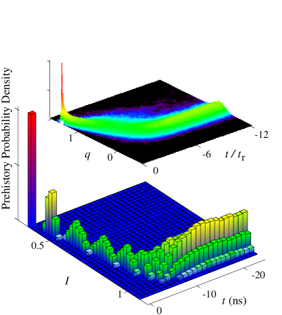
FIG. 2.: (color) The prehistory probability distribution of the scaled radiation intensity $I$ for experimentally observed dropout events in a semiconductor laser. Inset: the PPD for a Brownian particle, obtained from simulations for the same parameters as in Fig. 1.

As $-t$ increases further, the peak of the distribution (7) approaches the diffusion region $|q-q_{a}|\sim(Dt_{r})^{1/2}$ near the potential minimum, and the peak width (8) again shrinks down. For large $-t$, the PPD (3) goes over into the stationary distribution $\rho(q)$, which has a nearly Gaussian peak at $q_{a}$ with variance $Dt_{r}/2$.

We note that, in the most interesting region C, the positions of the maxima of $p_{h}$ (7) with respect to $q$ for given $t$ and with respect to $t$ for given $q$ are different. This indicates that there is no well-defined most probable escape path in space and time, which would go from the metastable state all the way over the barrier top. Still one can tell when the escaped system passed, most probably, through a given point, and where the system was most probably located at a given time.

The discussed qualitative features of the prehistory distribution can be seen from the results of digital simulations for the model potential

$$U(q)=q^{2}/2-q^{3}/3,$$ (9)

The data were obtained using a standard algorithm [15], and refer to 8000 events.

A distinct peak of the simulated $p_{h}$ is seen in Fig. 2. The peak of $p_{h}$ as a function of $q$ changes with increasing $|t|$ from a narrow Gaussian near $q_{f}$ to a broad and asymmetric between $q_{a}$ and $q_{b}$, and then again to a comparatively narrow Gaussian near $q_{a}$. The positions of the peak of $p_{h}$ with respect to time, $t_{m}(q)$, and coordinate, $q_{m}(t)$, are compared in Fig. 1. Both curves are close to each other. Outside the well they practically coincide and closely follow the noise-free path of the system, $dt_{m}/dq=-1/U^{\prime}(q)$. The motion displays a characteristic slowing down near the barrier top. Inside the well the peak moves close to the optimal fluctuational path $\dot{q}=U^{\prime}(q)$. The distribution $p_{h}$ becomes time-independent for large $|t|$. Therefore $t_{m}(q)$ is well-defined only for $q$ not too close to the potential minimum $q_{a}$.

The data of simulations in Figs. 1, 2 refer to the noise intensities $D/\Delta U=0.1$, where the asymptotic analytical theory applies only qualitatively. In particular, the expressions (4) and (7) for $p_{h}$ in different ranges of $q$ do not merge with each other smoothly, as seen from Fig. 1. However, there is good qualitative agreement between the analytical and numerical data, including the position of the peak and the integral width of the PPD.

Numerical results on the standard deviation of the PPD $\sigma$ for two noise intensities are shown in Fig. 3. As expected, the distribution width reaches its maximum well inside the well, near the inflection point $U^{\prime\prime}(q)=0$. For higher $D$, the maximum is less pronounced.

FIG. 3.: Standard deviation and the position of the maximum of the prehistory distribution at given time, for simulated Brownian motion (left panel) and a semiconductor laser with optical feedback (right panel). Solid and dashed lines on the left panel refer to $\Delta U/D=10$ and 3, respectively. The scales in the panels are different (see the text).

The experimental observation of the prehistory distribution was made using a semiconductor laser with optical feedback. The setup was similar to that used before [16] and consisted of a temperature-stabilized laser diode and a remote flat-surface mirror. The feedback could be controlled by a variable attenuator between them. Near the solitary laser threshold, such a system is unstable: after some time of nearly steady operation the radiation intensity drops down, then it comparatively fast recovers to the original value, then drops down again, etc. In the experiment, the intensity output was digitized, with time resolution 1 ns. To obtain the prehistory distribution, the intensity records were superimposed backward in time, starting from the instant at which the intensity, on its way down, reached a certain level (10% above the extreme dropout point). The PPD obtained from 1512 events for the feedback 15.63% is shown in Fig. 2.

The mechanism of power dropouts is vividly discussed in the literature [16, 3, 17, 18, 19]. Most authors agree that the role of noise in this effect is crucial. A simple model [20] describes the dropouts in terms of activation escape of the light intensity $I$ over a potential barrier with shape (9). Previous observations [16] were in agreement with this model, which motivated us to measure the prehistory distribution for dropout events.

It is seen from Figs. 2 and 3 that the results of the observations agree with major qualitative results on noise-induced escape. The experimental PPD displays a distinct peak. The shape of this peak is similar to the shape of the PPD of a noise-driven system, with the light intensity $I$ playing the role of the coordinate $q$ ($I$ is scaled by its metastable value). The peak is narrow at small time $|t|$, and displays a characteristic broadening at intermediate times. For larger $|t|$, the peak becomes time-independent. From the data in Figs. 2 and 3, the relaxation time of the system is $t_{r}\approx 2$ ns. From the value of the escape rate $W\approx 5\times 10^{-3}$ ns^-1 found in [16], it follows that, for the model  (9), $\Delta U/D\approx 3$. Using an estimate $\sigma_{0}\approx(D/U^{\prime\prime}(q_{a}))^{1/2}$ for $\sigma$ at large $-t$, one can estimate the difference $6(\Delta U/D)^{1/2}\sigma_{0}$ in the light intensity $I$ at the minimum and maximum of the potential (9). It then follows from Fig. 3b that the system goes through the potential maximum for $t\sim-4$ ns, i.e. the width $\sigma$ reaches its maximum near the potential maximum. In combination with larger $\sigma_{\max}/\sigma_{0}$ compared to that in Fig. 3a for the same $\Delta U/D$, this indicates that the model (1), (9) is oversimplified. However, the overall form of the PPD seen from the data provides an important argument in favor of the stochastic model of dropout events. We expect that it will be possible to use high-resolution data on the prehistory distribution in order to establish a quantitative model of the system.

In conclusion, we have analyzed the dynamics of a system in activated escape and revealed its distinctive features related to the occurrence of optimal paths and to the motion slowing down near a barrier top. The escape trajectories lie within a well-defined tube, and the system is most likely to go through a cross-section of this tube at a well-defined time before it is found behind the barrier. For the first time, a tube of escape trajectories has been observed in experiment, by analyzing dropout events in a semiconductor laser.

The work at MSU was partly supported from the NSF funded MRSEC and the NSF grants no. PHY-9722057 and no. DMR-9809688.

REFERENCES

- [1] e-mail: dykman@pa.msu.edu
- [2] R. Roy, R. Short, J. Durnin, and L. Mandel, Phys. Rev. Lett. 45, 1486 (1980); M. B. Willimsen et al., Phys. Rev. Lett. 82, 4815 (1999).
- [3] A. M. Yacomotti et al., Phys. Rev. Lett. 83, 292 (1999).
- [4] L.J. Lapidus, D. Enzer, and G. Gabrielse, Phys. Rev. Lett. 83, 899 (1999); M.I. Dykman, C.M. Maloney, V.N. Smelyanskiy, and M. Silverstein, Phys. Rev. E 57, 5202 (1998).
- [5] D.G. Luchinsky, P.V.E. McClintock, and M.I. Dykman, Rep. Progr. Phys. 61, 889 (1998).
- [6] M.I. Dykman et al., Nuovo Cimento D 17, 661 (1995); L. Gammaitoni et al., Rev. Mod. Phys. 70, 223 (1998); R.D. Astumian and F. Moss, Chaos 8, 533 (1998); K. Wiesenfeld and F. Jaramillo, Chaos 8, 539 (1998).
- [7] L. Onsager and S. Machlup, Phys. Rev. 91, 1505 (1953).
- [8] M. I. Freidlin and A. D. Wentzel, Random Perturbations in Dynamical Systems (Springer, New-York, 1984); R. Graham, in Noise in Nonlinear Dynamical Systems, edited by F. Moss and P.V.E. McClintock (Cambridge University, Cambridge, 1989), v. 1, p. 225; M.I. Dykman, M.A. Krivoglaz, and S.M. Soskin, ibid., v. 2, p. 347.
- [9] M.I. Dykman et al., Phys. Rev. Lett. 68, 2718 (1992).
- [10] A peak in the prehistory distribution for lying at the top of a potential barrier, was seen in analog simulations (P.V.E. McClintock, private communication).
- [11] M. Suzuki, J. Stat. Phys. 16, 11, 477 (1977).
- [12] N.G. van Kampen, Stochastic Processes in Physics and Chemistry (Elsevier, Amsterdam 1981).
- [13] In contrast to the present case, in the standard analysis [5, 8] of interest are the optimal paths that start from the attractor and end at a given state.
- [14] A. Zhukov and M.I. Dykman, in preparation.
- [15] R. Mannella, in Supercomputation in Nonlinear and Disordered Systems, edited by L. Vázquez, F. Tirando, and I. Martin (World Scientific, Singapore, 1997), p. 100.
- [16] A. Hohl, H.J.C. van der Linden, and R. Roy, Opt. Lett. 20, 2396 (1995).
- [17] G. Huyet et al., Europhys. Lett. 40, 619 (1997); G. Huyet et al., Opt. Comm. 149, 341 (1998).
- [18] G. Vaschenko et al., Phys. Rev. Lett. 81, 5536 (1998).
- [19] A. Hohl and A. Gavrielides, Phys. Rev. Lett. 82, 1148 (1999).
- [20] C.H. Henry and R.F. Kazarinov, IEEE J. Quantum Electron. QE-22, 294 (1986).