Effect of Magnetic Impurities on Suppression of the Transition Temperature in Disordered Superconductors

Robert A Smith School of Physics and Astronomy, University of Birmingham, Edgbaston, Birmingham B15 2TT, England and Laboratory of Atomic and Solid State Physics, Cornell University, Ithaca, New York 14853    Vinay Ambegaokar Laboratory of Atomic and Solid State Physics, Cornell University, Ithaca, New York 14853
Abstract

We calculate the first-order perturbative correction to the transition temperature $T_{c}$ in a superconductor with both non-magnetic and magnetic impurities. We do this by first evaluating the correction to the effective potential, $\Omega(\Delta)$, and then obtain the first-order correction to order parameter, $\Delta$, by finding the minimum of $\Omega(\Delta)$. Setting $\Delta=0$ finally enables $T_{c}$ to be evaluated. $T_{c}$ is now a function of both the resistance per square, RΒ Β Β Β Β subscript𝑅     R_{\mathchoice{\vbox{\vbox{\hrule height=0.4pt\hbox{\vrule width=0.4pt,height=3.0pt\kern 3.0pt\vrule width=0.4pt} \hrule height=0.4pt}}}{\vbox{\vbox{\hrule height=0.4pt\hbox{\vrule width=0.4pt,height=3.0pt\kern 3.0pt\vrule width=0.4pt} \hrule height=0.4pt}}}{\vbox{\vbox{\hrule height=0.3pt\hbox{\vrule width=0.3pt,height=2.1pt\kern 2.1pt\vrule width=0.3pt} \hrule height=0.3pt}}}{\vbox{\vbox{\hrule height=0.3pt\hbox{\vrule width=0.3pt,height=1.5pt\kern 1.5pt\vrule width=0.3pt} \hrule height=0.3pt}}}}, a measure of the non-magnetic disorder, and the spin-flip scattering rate, 1/Ο„s1subscriptπœπ‘ 1/\tau_{s}, a measure of magnetic disorder. We find that the effective pair-breaking rate per magnetic impurity is virtually independent of the resistance per square of the film, in agreement with an experiment of Chervenak and Valles. This conclusion is supported both by the perturbative calculation, and by a non-perturbative re-summation technique.


I Introduction

Many experiments[1] performed on homogeneous disordered thin film superconductors have shown that superconductivity is suppressed by increasing disorder, as measured by the normal state resistance per square, RΒ Β Β Β Β subscript𝑅     R_{\mathchoice{\vbox{\vbox{\hrule height=0.4pt\hbox{\vrule width=0.4pt,height=3.0pt\kern 3.0pt\vrule width=0.4pt} \hrule height=0.4pt}}}{\vbox{\vbox{\hrule height=0.4pt\hbox{\vrule width=0.4pt,height=3.0pt\kern 3.0pt\vrule width=0.4pt} \hrule height=0.4pt}}}{\vbox{\vbox{\hrule height=0.3pt\hbox{\vrule width=0.3pt,height=2.1pt\kern 2.1pt\vrule width=0.3pt} \hrule height=0.3pt}}}{\vbox{\vbox{\hrule height=0.3pt\hbox{\vrule width=0.3pt,height=1.5pt\kern 1.5pt\vrule width=0.3pt} \hrule height=0.3pt}}}}. The majority of the data is of the transition temperature as a function of the resistance per square, Tc​(RΒ Β Β Β Β )subscript𝑇𝑐subscript𝑅     T_{c}(R_{\mathchoice{\vbox{\vbox{\hrule height=0.4pt\hbox{\vrule width=0.4pt,height=3.0pt\kern 3.0pt\vrule width=0.4pt} \hrule height=0.4pt}}}{\vbox{\vbox{\hrule height=0.4pt\hbox{\vrule width=0.4pt,height=3.0pt\kern 3.0pt\vrule width=0.4pt} \hrule height=0.4pt}}}{\vbox{\vbox{\hrule height=0.3pt\hbox{\vrule width=0.3pt,height=2.1pt\kern 2.1pt\vrule width=0.3pt} \hrule height=0.3pt}}}{\vbox{\vbox{\hrule height=0.3pt\hbox{\vrule width=0.3pt,height=1.5pt\kern 1.5pt\vrule width=0.3pt} \hrule height=0.3pt}}}})[2, 3, 4, 5], although there is some data on the upper critical field, Hc​2​(T,RΒ Β Β Β Β )subscript𝐻𝑐2𝑇subscript𝑅     H_{c2}(T,R_{\mathchoice{\vbox{\vbox{\hrule height=0.4pt\hbox{\vrule width=0.4pt,height=3.0pt\kern 3.0pt\vrule width=0.4pt} \hrule height=0.4pt}}}{\vbox{\vbox{\hrule height=0.4pt\hbox{\vrule width=0.4pt,height=3.0pt\kern 3.0pt\vrule width=0.4pt} \hrule height=0.4pt}}}{\vbox{\vbox{\hrule height=0.3pt\hbox{\vrule width=0.3pt,height=2.1pt\kern 2.1pt\vrule width=0.3pt} \hrule height=0.3pt}}}{\vbox{\vbox{\hrule height=0.3pt\hbox{\vrule width=0.3pt,height=1.5pt\kern 1.5pt\vrule width=0.3pt} \hrule height=0.3pt}}}})[3, 6, 7], and the order parameter Δ​(RΒ Β Β Β Β )Ξ”subscript𝑅     \Delta(R_{\mathchoice{\vbox{\vbox{\hrule height=0.4pt\hbox{\vrule width=0.4pt,height=3.0pt\kern 3.0pt\vrule width=0.4pt} \hrule height=0.4pt}}}{\vbox{\vbox{\hrule height=0.4pt\hbox{\vrule width=0.4pt,height=3.0pt\kern 3.0pt\vrule width=0.4pt} \hrule height=0.4pt}}}{\vbox{\vbox{\hrule height=0.3pt\hbox{\vrule width=0.3pt,height=2.1pt\kern 2.1pt\vrule width=0.3pt} \hrule height=0.3pt}}}{\vbox{\vbox{\hrule height=0.3pt\hbox{\vrule width=0.3pt,height=1.5pt\kern 1.5pt\vrule width=0.3pt} \hrule height=0.3pt}}}})[8, 9]. The main data to be explained thus consists of Tc​(RΒ Β Β Β Β )subscript𝑇𝑐subscript𝑅     T_{c}(R_{\mathchoice{\vbox{\vbox{\hrule height=0.4pt\hbox{\vrule width=0.4pt,height=3.0pt\kern 3.0pt\vrule width=0.4pt} \hrule height=0.4pt}}}{\vbox{\vbox{\hrule height=0.4pt\hbox{\vrule width=0.4pt,height=3.0pt\kern 3.0pt\vrule width=0.4pt} \hrule height=0.4pt}}}{\vbox{\vbox{\hrule height=0.3pt\hbox{\vrule width=0.3pt,height=2.1pt\kern 2.1pt\vrule width=0.3pt} \hrule height=0.3pt}}}{\vbox{\vbox{\hrule height=0.3pt\hbox{\vrule width=0.3pt,height=1.5pt\kern 1.5pt\vrule width=0.3pt} \hrule height=0.3pt}}}}) curves for different materials. To see how disorder might affect $T_{c}$, consider the mean field equation,

$$T_{c0}=1.13\omega_{D}\exp{\left[-{1\over N(0)(\lambda-\mu^{*})}\right]},$$ (1)

where $\lambda$ is the attractive BCS interaction mediated by phonons of energy less than the Debye frequency, $\omega_{D}$, $\mu^{*}$ is the Coulomb pseudopotential, the effective strength of the Coulomb repulsion, and $N(0)$ is the single particle density of states at the Fermi surface. Obviously disorder could affect $T_{c}$ by changing $\lambda$, $\mu^{*}$, and $N(0)$. In particular the diffusive motion of electrons caused by the disorder is known to lead to an increased effective strength of the Coulomb interaction, as the screening is less efficient than with ballistic electrons, and this leads to an increase in $\mu^{*}$, and a decrease in $N(0)$. Calculating the first-order perturbative correction caused by the disorder shows that we must consider all these processes together[10, 11]. This is because the disorder-screened Coulomb interaction has a low-momentum singularity which leads to the separate effects being large; however, when they are added together this singularity is cancelled, and the actual effect is much smaller than might be naively expected. The final result has the form

ln⁑(TcTc​0)=βˆ’13​RΒ Β Β Β Β R0​ln3⁑(12​π​Tc​0​τ),subscript𝑇𝑐subscript𝑇𝑐013subscript𝑅     subscript𝑅0superscript312πœ‹subscript𝑇𝑐0𝜏\ln{\left({T_{c}\over T_{c0}}\right)}=-{1\over 3}{R_{\mathchoice{\vbox{\vbox{\hrule height=0.4pt\hbox{\vrule width=0.4pt,height=3.0pt\kern 3.0pt\vrule width=0.4pt} \hrule height=0.4pt}}}{\vbox{\vbox{\hrule height=0.4pt\hbox{\vrule width=0.4pt,height=3.0pt\kern 3.0pt\vrule width=0.4pt} \hrule height=0.4pt}}}{\vbox{\vbox{\hrule height=0.3pt\hbox{\vrule width=0.3pt,height=2.1pt\kern 2.1pt\vrule width=0.3pt} \hrule height=0.3pt}}}{\vbox{\vbox{\hrule height=0.3pt\hbox{\vrule width=0.3pt,height=1.5pt\kern 1.5pt\vrule width=0.3pt} \hrule height=0.3pt}}}}\over R_{0}}\ln^{3}{\left({1\over 2\pi T_{c0}\tau}\right)}, (2)

where $R_{0}=2\pi h/e^{2}\approx 162k\Omega$ and $\tau$ is the elastic scattering time. We see that this curve is essentially β€œuniversal”, depending on only a single fitting parameter, $\beta=\ln{(1/2\pi T_{c0}\tau)}$. Experimentally it is found that Tc​(RΒ Β Β Β Β )subscript𝑇𝑐subscript𝑅     T_{c}(R_{\mathchoice{\vbox{\vbox{\hrule height=0.4pt\hbox{\vrule width=0.4pt,height=3.0pt\kern 3.0pt\vrule width=0.4pt} \hrule height=0.4pt}}}{\vbox{\vbox{\hrule height=0.4pt\hbox{\vrule width=0.4pt,height=3.0pt\kern 3.0pt\vrule width=0.4pt} \hrule height=0.4pt}}}{\vbox{\vbox{\hrule height=0.3pt\hbox{\vrule width=0.3pt,height=2.1pt\kern 2.1pt\vrule width=0.3pt} \hrule height=0.3pt}}}{\vbox{\vbox{\hrule height=0.3pt\hbox{\vrule width=0.3pt,height=1.5pt\kern 1.5pt\vrule width=0.3pt} \hrule height=0.3pt}}}}) curves from a wide variety of materials fit well to this equation, or extensions of it that allow for stronger disorder. The simplest extension simply consists of replacing $T_{c0}$ by $T_{c}$ on the right-hand side of Eq. (2), which leads to the cubic equation

$$x={t\over 3}(\beta+x)^{3},$$ (3)

where $x=\ln{(T_{c0}/T_{c})}$ and t=RΒ Β Β Β Β /R0𝑑subscript𝑅     subscript𝑅0t=R_{\mathchoice{\vbox{\vbox{\hrule height=0.4pt\hbox{\vrule width=0.4pt,height=3.0pt\kern 3.0pt\vrule width=0.4pt} \hrule height=0.4pt}}}{\vbox{\vbox{\hrule height=0.4pt\hbox{\vrule width=0.4pt,height=3.0pt\kern 3.0pt\vrule width=0.4pt} \hrule height=0.4pt}}}{\vbox{\vbox{\hrule height=0.3pt\hbox{\vrule width=0.3pt,height=2.1pt\kern 2.1pt\vrule width=0.3pt} \hrule height=0.3pt}}}{\vbox{\vbox{\hrule height=0.3pt\hbox{\vrule width=0.3pt,height=1.5pt\kern 1.5pt\vrule width=0.3pt} \hrule height=0.3pt}}}}/R_{0}. This equation shows unphysical reentrance at strong disorder, an artefact which is removed by either a renormalization group treatment[10], or the use of a non-perturbative resummation technique[12] to yield the formula

$$\ln{\left({T_{c}\over T_{c0}}\right)}={1\over\lambda}-{1\over 2\sqrt{t}}\ln{\left({1+\sqrt{t}/\lambda\over 1-\sqrt{t}/\lambda}\right)}.$$ (4)

The fact that most data can be fit to a single curve is pleasing in that it shows that the basic ingredients of our theory – disorder, BCS attraction and Coulomb repulsion – are correct. However it does not allow analysis of the sensitivity of the theory or experiment to changes in details of the system, such as the exact form of the phonon-mediated attraction. Moreover there are other theories[13] which posit the importance of such details which give predictions that are equally in agreement with experiment. We see that the Tc​(RΒ Β Β Β Β )subscript𝑇𝑐subscript𝑅     T_{c}(R_{\mathchoice{\vbox{\vbox{\hrule height=0.4pt\hbox{\vrule width=0.4pt,height=3.0pt\kern 3.0pt\vrule width=0.4pt} \hrule height=0.4pt}}}{\vbox{\vbox{\hrule height=0.4pt\hbox{\vrule width=0.4pt,height=3.0pt\kern 3.0pt\vrule width=0.4pt} \hrule height=0.4pt}}}{\vbox{\vbox{\hrule height=0.3pt\hbox{\vrule width=0.3pt,height=2.1pt\kern 2.1pt\vrule width=0.3pt} \hrule height=0.3pt}}}{\vbox{\vbox{\hrule height=0.3pt\hbox{\vrule width=0.3pt,height=1.5pt\kern 1.5pt\vrule width=0.3pt} \hrule height=0.3pt}}}}) curves alone are not enough to allow consideration of the relative merits of different theories. What we would like to do is to add some additional parameter to the experimental system to give a whole new set of data – for example a family of Tc​(RΒ Β Β Β Β )subscript𝑇𝑐subscript𝑅     T_{c}(R_{\mathchoice{\vbox{\vbox{\hrule height=0.4pt\hbox{\vrule width=0.4pt,height=3.0pt\kern 3.0pt\vrule width=0.4pt} \hrule height=0.4pt}}}{\vbox{\vbox{\hrule height=0.4pt\hbox{\vrule width=0.4pt,height=3.0pt\kern 3.0pt\vrule width=0.4pt} \hrule height=0.4pt}}}{\vbox{\vbox{\hrule height=0.3pt\hbox{\vrule width=0.3pt,height=2.1pt\kern 2.1pt\vrule width=0.3pt} \hrule height=0.3pt}}}{\vbox{\vbox{\hrule height=0.3pt\hbox{\vrule width=0.3pt,height=1.5pt\kern 1.5pt\vrule width=0.3pt} \hrule height=0.3pt}}}}) curves for a single material as this new parameter is altered. Chervenak and Valles[14] have recently performed an experiment of this type in which magnetic $Gd$ impurities are added to thin films of $Pb_{0.9}Bi_{0.1}$. This introduces the new feature of spin-flip scattering to the system, which is measured by the spin-flip scattering rate, 1/Ο„s1subscriptπœπ‘ 1/\tau_{s}. The task of the theorist is to now make predictions for $T_{c}$ as a function of both RΒ Β Β Β Β subscript𝑅     R_{\mathchoice{\vbox{\vbox{\hrule height=0.4pt\hbox{\vrule width=0.4pt,height=3.0pt\kern 3.0pt\vrule width=0.4pt} \hrule height=0.4pt}}}{\vbox{\vbox{\hrule height=0.4pt\hbox{\vrule width=0.4pt,height=3.0pt\kern 3.0pt\vrule width=0.4pt} \hrule height=0.4pt}}}{\vbox{\vbox{\hrule height=0.3pt\hbox{\vrule width=0.3pt,height=2.1pt\kern 2.1pt\vrule width=0.3pt} \hrule height=0.3pt}}}{\vbox{\vbox{\hrule height=0.3pt\hbox{\vrule width=0.3pt,height=1.5pt\kern 1.5pt\vrule width=0.3pt} \hrule height=0.3pt}}}} (the measure of non-magnetic disorder), and 1/Ο„s1subscriptπœπ‘ 1/\tau_{s}, (the measure of magnetic disorder), and to compare these to experiment.

In this paper we calculate the first-order perturbative correction to the transition temperature, $T_{c}$, of a superconductor with both non-magnetic and magnetic impurities. The model used consists of a featureless BCS attraction, $-\lambda$, and a Coulomb repulsion, $V_{C}(q)$, between electrons which scatter off non-magnetic and magnetic impurities. The model is the simplest one that contains the essential physics, and its shortcoming of not considering the details of the attractive interaction is offset by the fact that we can consider all processes to a given order of perturbation theory. This is an important consideration in view of the cancellation of low-momentum singularities in the screened Coulomb potential discussed in the opening paragraph. In fact, an obvious question is whether this cancellation persists in the presence of magnetic impurities. We find that this is indeed the case, and so the details of the screened Coulomb interaction are removed, leading to a β€œuniversal” form for Tc​(RΒ Β Β Β Β ,1/Ο„s)subscript𝑇𝑐subscript𝑅     1subscriptπœπ‘ T_{c}(R_{\mathchoice{\vbox{\vbox{\hrule height=0.4pt\hbox{\vrule width=0.4pt,height=3.0pt\kern 3.0pt\vrule width=0.4pt} \hrule height=0.4pt}}}{\vbox{\vbox{\hrule height=0.4pt\hbox{\vrule width=0.4pt,height=3.0pt\kern 3.0pt\vrule width=0.4pt} \hrule height=0.4pt}}}{\vbox{\vbox{\hrule height=0.3pt\hbox{\vrule width=0.3pt,height=2.1pt\kern 2.1pt\vrule width=0.3pt} \hrule height=0.3pt}}}{\vbox{\vbox{\hrule height=0.3pt\hbox{\vrule width=0.3pt,height=1.5pt\kern 1.5pt\vrule width=0.3pt} \hrule height=0.3pt}}}},1/\tau_{s}).

The main result of the paper is that the pair-breaking rate per magnetic impurity, α′​(RΒ Β Β Β Β )superscript𝛼′subscript𝑅     \alpha^{\prime}(R_{\mathchoice{\vbox{\vbox{\hrule height=0.4pt\hbox{\vrule width=0.4pt,height=3.0pt\kern 3.0pt\vrule width=0.4pt} \hrule height=0.4pt}}}{\vbox{\vbox{\hrule height=0.4pt\hbox{\vrule width=0.4pt,height=3.0pt\kern 3.0pt\vrule width=0.4pt} \hrule height=0.4pt}}}{\vbox{\vbox{\hrule height=0.3pt\hbox{\vrule width=0.3pt,height=2.1pt\kern 2.1pt\vrule width=0.3pt} \hrule height=0.3pt}}}{\vbox{\vbox{\hrule height=0.3pt\hbox{\vrule width=0.3pt,height=1.5pt\kern 1.5pt\vrule width=0.3pt} \hrule height=0.3pt}}}}), defined by

α′​(RΒ Β Β Β Β )=Tc​(RΒ Β Β Β Β ,0)βˆ’Tc​(RΒ Β Β Β Β ,1/Ο„s)1/Ο„ssuperscript𝛼′subscript𝑅     subscript𝑇𝑐subscript𝑅     0subscript𝑇𝑐subscript𝑅     1subscriptπœπ‘ 1subscriptπœπ‘ \alpha^{\prime}(R_{\mathchoice{\vbox{\vbox{\hrule height=0.4pt\hbox{\vrule width=0.4pt,height=3.0pt\kern 3.0pt\vrule width=0.4pt} \hrule height=0.4pt}}}{\vbox{\vbox{\hrule height=0.4pt\hbox{\vrule width=0.4pt,height=3.0pt\kern 3.0pt\vrule width=0.4pt} \hrule height=0.4pt}}}{\vbox{\vbox{\hrule height=0.3pt\hbox{\vrule width=0.3pt,height=2.1pt\kern 2.1pt\vrule width=0.3pt} \hrule height=0.3pt}}}{\vbox{\vbox{\hrule height=0.3pt\hbox{\vrule width=0.3pt,height=1.5pt\kern 1.5pt\vrule width=0.3pt} \hrule height=0.3pt}}}})={T_{c}(R_{\mathchoice{\vbox{\vbox{\hrule height=0.4pt\hbox{\vrule width=0.4pt,height=3.0pt\kern 3.0pt\vrule width=0.4pt} \hrule height=0.4pt}}}{\vbox{\vbox{\hrule height=0.4pt\hbox{\vrule width=0.4pt,height=3.0pt\kern 3.0pt\vrule width=0.4pt} \hrule height=0.4pt}}}{\vbox{\vbox{\hrule height=0.3pt\hbox{\vrule width=0.3pt,height=2.1pt\kern 2.1pt\vrule width=0.3pt} \hrule height=0.3pt}}}{\vbox{\vbox{\hrule height=0.3pt\hbox{\vrule width=0.3pt,height=1.5pt\kern 1.5pt\vrule width=0.3pt} \hrule height=0.3pt}}}},0)-T_{c}(R_{\mathchoice{\vbox{\vbox{\hrule height=0.4pt\hbox{\vrule width=0.4pt,height=3.0pt\kern 3.0pt\vrule width=0.4pt} \hrule height=0.4pt}}}{\vbox{\vbox{\hrule height=0.4pt\hbox{\vrule width=0.4pt,height=3.0pt\kern 3.0pt\vrule width=0.4pt} \hrule height=0.4pt}}}{\vbox{\vbox{\hrule height=0.3pt\hbox{\vrule width=0.3pt,height=2.1pt\kern 2.1pt\vrule width=0.3pt} \hrule height=0.3pt}}}{\vbox{\vbox{\hrule height=0.3pt\hbox{\vrule width=0.3pt,height=1.5pt\kern 1.5pt\vrule width=0.3pt} \hrule height=0.3pt}}}},1/\tau_{s})\over 1/\tau_{s}} (5)

is roughly independent of RΒ Β Β Β Β subscript𝑅     R_{\mathchoice{\vbox{\vbox{\hrule height=0.4pt\hbox{\vrule width=0.4pt,height=3.0pt\kern 3.0pt\vrule width=0.4pt} \hrule height=0.4pt}}}{\vbox{\vbox{\hrule height=0.4pt\hbox{\vrule width=0.4pt,height=3.0pt\kern 3.0pt\vrule width=0.4pt} \hrule height=0.4pt}}}{\vbox{\vbox{\hrule height=0.3pt\hbox{\vrule width=0.3pt,height=2.1pt\kern 2.1pt\vrule width=0.3pt} \hrule height=0.3pt}}}{\vbox{\vbox{\hrule height=0.3pt\hbox{\vrule width=0.3pt,height=1.5pt\kern 1.5pt\vrule width=0.3pt} \hrule height=0.3pt}}}} except near the superconductor-insulator transition, in agreement with experiment. This is confirmed both by first-order perturbation theory, and also by a non-perturbative resummation technique which we introduce to remove concerns about reentrance problems at stronger disorder. This agreement of the two theoretical approaches with each other and the experimental data gives us confidence in our results.

To calculate the correction to $T_{c}$ we use a collective mode formalism derived in a previous paper[11] (which we refer to as I from now on) on the suppression of $\Delta$ by non-magnetic disorder. The introduction of magnetic impurities means that we have to modify the formalism somewhat, and so we include most of the derivation in this paper. The method used in this paper to evaluate the correction to $T_{c}$ proceeds in three stages. First we find the first-order correction to the grand canonical potential, $\Omega_{1}(\Delta)$, of the superconductor due to fluctuations of its collective modes. Then by minimizing the total grand canonical potential, $\Omega_{0}(\Delta)+\Omega_{1}(\Delta)$ with respect to the order parameter, $\Delta$, we obtain the first-order correction to the order parameter self-consistency equation. Finally by setting $\Delta=0$ we obtain the first-order correction to transition temperature $T_{c}$. The method we use has the advantage that it is impossible to β€œmiss diagrams” since there is only one diagram in the $\Omega_{1}(\Delta)$ calculation, and we also obtain the equation for $\Delta$ at no extra cost. The equations for $T_{c}$ and $\Delta$ must reduce to those of I when we set spin-flip scattering to zero, providing a useful consistency check. A key result of the calculation in I was that the singularity in the screened Coulomb potential persists below $T_{c}$, and that this singularity is cancelled in the formula for the suppression of $\Delta$ in a similar manner to the cancellation in the formula for $T_{c}$. Therefore an important question is whether this singularity and cancellation remains when magnetic impurities are added. We show that this is indeed the case, and moreover that the cancellation is due to gauge invariance, and will occur in first-order perturbation theory in the presence of any kind of impurity scattering. In other words, it is not possible to obtain stronger suppression of the transition temperature by introducing some exotic scattering mechanism. It is also reassuring to know that an otherwise mysterious cancellation between diagrams has its physical origin in gauge invariance, and we hope that similar arguments may be applied to show that the result holds to all orders in perturbation theory.

The outline of the rest of the paper is as follows. In section II we derive the matrix formalism for superconductors with magnetic impurities, and the collective mode approach we will use. We derive the RPA screened bosonic propagators, and show that low-momentum singularities persist in the screened Coulomb propagator below $T_{c}$. In section III we derive the first order perturbative correction to the grand canonical potential $\Omega_{1}(\Delta)$, and from this the correction to the order parameter $\Delta$. In section IV we set $\Delta=0$ to obtain the correction to transition temperature $T_{c}$. In section V we calculate $T_{c}$ numerically using both the perturbative results of section IV and a recently developed non-pertubative technique, and compare to experiment.

II Derivation of the $4\times 4$ Matrix Formalism

Superconductivity with Magnetic Impurities:

We consider a system of electrons that scatter off static non-magnetic and magnetic impurities, and interact with each other via the long-range Coulomb interaction and the BCS attraction. The scattering from static impurities is described by Hamiltonian

$$H_{e-i}=\sum_{\alpha\beta}\int d{\bf x}\psi^{+}_{\alpha}({\bf x})\left\{\left[-{\nabla^{2}_{x}\over 2m}+\sum_{i}u_{0}({\bf x}-{\bf x_{i}})\right]\delta_{\alpha\beta}+\sum_{j}J({\bf x-x_{j}}){\bf S_{j}\cdot\sigma_{\alpha\beta}}\right\}\psi_{\beta}({\bf x}),$$ (6)

where $\psi^{+}_{\alpha}$, $\psi_{\alpha}$ are the electron creation and annhilation operators, $u_{0}({\bf x}-{\bf x_{i}})$ is the impurity potential at ${\bf x}$ due to a non-magnetic impurity at ${\bf x_{i}}$, ${\bf S_{j}}$ is a magnetic impurity spin moment at ${\bf x_{j}}$, and $J({\bf x})$ is the electron-impurity exchange coupling. The potential and spin-flip scattering rates are then given by

$\displaystyle{1\over\tau_{0}}$ $\displaystyle=$ $\displaystyle 2\pi N(0)n_{i}|u_{0}|^{2}$ (7)
1Ο„s1subscriptπœπ‘ \displaystyle{1\over\tau_{s}} $\displaystyle=$ $\displaystyle 2\pi N(0)n_{j}J^{2}S(S+1),$ (8)

where $u_{0}$ is the Fourier transform of $u_{0}({\bf x})$, and $J$ is the Fourier transform of $J({\bf x})$, both assumed independent of momentum, $n_{i}$ is the non-magnetic impurity density, and $n_{j}$ the magnetic impurity density.

The Coulomb repulsion between electrons is described by Hamiltonian

$$H_{C}=\sum_{\alpha\beta}\int d{\bf x}\int d{\bf x^{\prime}}\psi^{+}_{\alpha}({\bf x})\psi_{\alpha}({\bf x}){e^{2}\over|{\bf x}-{\bf x^{\prime}}|}\psi^{+}_{\beta}({\bf x^{\prime}})\psi_{\beta}({\bf x^{\prime}}),$$ (9)

leading to a bare Coulomb propagator that is just the Fourier transform of the above potential.

The BCS attraction is described by the Hamiltonian

$$H_{BCS}=-\lambda\sum_{\alpha\beta}\int d{\bf x}\psi^{+}_{\alpha}({\bf x})\psi_{\alpha}({\bf x})\psi^{+}_{\beta}({\bf x})\psi_{\beta}({\bf x}),$$ (10)

corresponding to an instantaneous contact interaction $-\lambda\delta({\bf x}-{\bf x^{\prime}})$.

Having introduced the model Hamiltonian we need to describe the system, we discuss the standard four-dimensional matrix representation[15] needed to describe a superconductor with magnetic impurities. We need four components to describe the two spin degrees of freedom, and the two types of correlation – the usual particle-hole correlation $<\psi_{\uparrow}\psi^{+}_{\uparrow}>$, amd the anomalous pairing correlation $<\psi_{\uparrow}\psi_{\downarrow}>$. We introduce the four-dimensional vector operator

$$\Psi=\left(\matrix{\psi_{\uparrow}\cr\psi_{\downarrow}\cr\psi^{+}_{\downarrow}\cr\psi^{+}_{\uparrow}\cr}\right)\quad;\quad\Psi^{+}=\left(\matrix{\psi^{+}_{\uparrow}&\psi^{+}_{\downarrow}&\psi_{\downarrow}&\psi_{\uparrow}\cr}\right),$$ (11)

with matrix propagator

$$<\Psi\Psi^{+}>=\left[\matrix{<\psi_{\uparrow}\psi^{+}_{\uparrow}>&<\psi_{\uparrow}\psi^{+}_{\downarrow}>&<\psi_{\uparrow}\psi_{\downarrow}>&<\psi_{\uparrow}\psi_{\uparrow}>\cr<\psi_{\downarrow}\psi^{+}_{\uparrow}>&<\psi_{\downarrow}\psi^{+}_{\downarrow}>&<\psi_{\downarrow}\psi_{\downarrow}>&<\psi_{\downarrow}\psi_{\uparrow}>\cr<\psi^{+}_{\downarrow}\psi^{+}_{\uparrow}>&<\psi^{+}_{\downarrow}\psi^{+}_{\downarrow}>&<\psi^{+}_{\downarrow}\psi_{\downarrow}>&<\psi^{+}_{\downarrow}\psi_{\uparrow}>\cr<\psi^{+}_{\uparrow}\psi^{+}_{\uparrow}>&<\psi^{+}_{\uparrow}\psi^{+}_{\downarrow}>&<\psi^{+}_{\uparrow}\psi_{\downarrow}>&<\psi^{+}_{\uparrow}\psi_{\uparrow}>\cr}\right].$$ (12)

In the normal state the temperature Green function is

$$G(k,i\omega)={1\over z-\varepsilon_{k}\tau_{3}\sigma_{0}},$$ (13)

where $z=i\omega$, $\omega=(2n+1)\pi T$ is a Fermi Matsubara frequency, and the $\tau_{i}$ and $\sigma_{i}$ are Pauli matrices operating on different spaces. The $\sigma_{i}$ operate in the usual spin space, whilst the $\tau_{i}$ operate in the Nambu (electron-hole) space. The diagrammatic rules are then the same as in the normal state except for the matrix structure of the Green function, and the presence of matrix $\tau_{3}\sigma_{0}$ at each interaction or impurity vertex due to the electron density operator being written in the form

$$\rho=\psi^{+}_{\uparrow}\psi_{\uparrow}+\psi^{+}_{\downarrow}\psi_{\downarrow}={1\over 2}\Psi^{+}\tau_{3}\sigma_{0}\Psi.$$ (14)

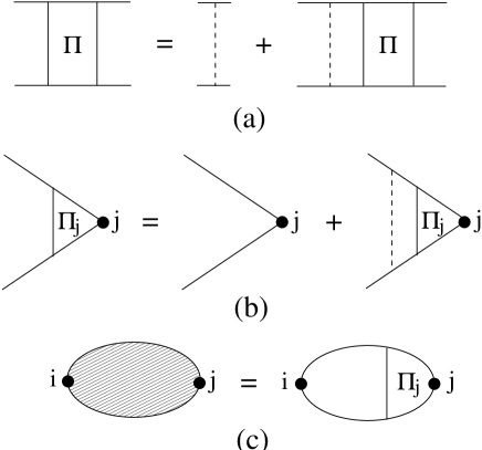
The pairing correlations in the clean superconductor can then be taken into account self-consistently as shown in Fig. (1a). Making the ansatz $\Sigma=\Delta\tau_{1}\sigma_{3}$ for the self-energy, the Green function for the pure superconductor becomes

$$G_{0}(k,z)={1\over z-\varepsilon_{k}\tau_{3}\sigma_{0}-\Delta\tau_{1}\sigma_{3}}={z+\varepsilon_{k}\tau_{3}\sigma_{0}+\Delta\tau_{1}\sigma_{3}\over z^{2}-\varepsilon_{k}^{2}-\Delta^{2}},$$ (15)

and the diagram of Fig. (1a) gives self-energy

$\displaystyle\Sigma\displaystyle$ $\displaystyle=$ $\displaystyle-\lambda T\sum_{\omega}N(0)\int d\varepsilon_{k}{\tau_{3}\sigma_{0}(z+\varepsilon_{k}\tau_{3}\sigma_{0}+\Delta\tau_{1}\sigma_{3})\tau_{3}\sigma_{0}\over\varepsilon_{k}^{2}-z^{2}+\Delta^{2}}$ (16)
$\displaystyle=$ $\displaystyle\displaystyle N(0)\lambda\Delta\tau_{1}\sigma_{3}T\sum_{\omega}{1\over\sqrt{\omega^{2}+\Delta^{2}}},$ (17)

which gives us the usual BCS self-consistency equation

$$1=N(0)\lambda T\sum_{\omega}{1\over\sqrt{\omega^{2}+\Delta^{2}}}.$$ (18)

We can treat the presence of non-magnetic and magnetic impurities by including an extra self-energy diagram to describe the dressing of the electron line by impurities as shown in Fig. (1b). We then make the ansatz that the pairing energy has the form $\Sigma_{p}=\Delta\tau_{1}\sigma_{3}$, and the impurity self-energy has the form $\Sigma_{imp}=-(\overline{z}-z)+(\overline{\Delta}-\Delta)\tau_{1}\sigma_{3}$, so that the Green function for the dirty superconductor is

$$G_{0}(k,z)={\overline{z}+\varepsilon_{k}\tau_{3}\sigma_{0}+\overline{\Delta}\tau_{1}\sigma_{3}\over\overline{z}^{2}-\varepsilon_{k}^{2}-\overline{\Delta}^{2}},$$ (19)

which is just the Green function for the clean superconductor with $z$, $\Delta$, replaced by $\overline{z}$, $\overline{\Delta}$, respectively. Since the impurity line has the form

Ξ“0=12​π​N​(0)​τ0​τ3​σ0βŠ—Ο„3​σ0+16​π​N​(0)​τs​[Ο„0​σ1βŠ—Ο„0​σ1+Ο„0​σ2βŠ—Ο„0​σ2+Ο„3​σ3βŠ—Ο„3​σ3],subscriptΞ“0tensor-product12πœ‹π‘0subscript𝜏0subscript𝜏3subscript𝜎0subscript𝜏3subscript𝜎016πœ‹π‘0subscriptπœπ‘ delimited-[]tensor-productsubscript𝜏0subscript𝜎1subscript𝜏0subscript𝜎1tensor-productsubscript𝜏0subscript𝜎2subscript𝜏0subscript𝜎2tensor-productsubscript𝜏3subscript𝜎3subscript𝜏3subscript𝜎3\Gamma_{0}={1\over 2\pi N(0)\tau_{0}}\tau_{3}\sigma_{0}\otimes\tau_{3}\sigma_{0}+{1\over 6\pi N(0)\tau_{s}}\left[\tau_{0}\sigma_{1}\otimes\tau_{0}\sigma_{1}+\tau_{0}\sigma_{2}\otimes\tau_{0}\sigma_{2}+\tau_{3}\sigma_{3}\otimes\tau_{3}\sigma_{3}\right], (20)

we obtain the self-consistency equation for $\overline{z}=i\overline{\omega}$ and $\overline{\Delta}$,

$$\overline{\omega}-\omega=\left({1\over 2\tau_{0}}+{1\over 2\tau_{s}}\right){\overline{\omega}\over\sqrt{\overline{\omega}^{2}+\overline{\Delta}^{2}}}\quad;\quad\overline{\Delta}-\Delta=\left({1\over 2\tau_{0}}-{1\over 2\tau_{s}}\right){\overline{\Delta}\over\sqrt{\overline{\omega}^{2}+\overline{\Delta}^{2}}}.$$ (21)

The diagrammatic definition of the pairing energy, $\Sigma_{p}$, leads to the same self-consistency equation for $\Delta$ as in the pure case except that $\omega$, $\Delta$, are replaced by $\overline{\omega}$, $\overline{\Delta}$. In the absence of magnetic impurities – i.e. 1/Ο„s=01subscriptπœπ‘ 01/\tau_{s}=0 – we see that $\overline{\omega}/\overline{\Delta}=\omega/\Delta$, and the equation for $\Delta$ is unchanged. This is Anderson’s theorem[16] that superconductivity is unaffected by non-magnetic impurities at mean-field level. In the presence of magnetic impurities we see that $\overline{\omega}/\overline{\Delta}\neq\omega/\Delta$, and if we define $u=\overline{\omega}/\overline{\Delta}$, ΞΆ=1/Ο„sβ€‹Ξ”πœ1subscriptπœπ‘ Ξ”\zeta=1/\tau_{s}\Delta, the problem reduces to solving the equation

$${\omega\over\Delta}=u\left(1-\zeta{1\over\sqrt{u^{2}+1}}\right).$$ (22)

The self-consistency equation for $\Delta$ then takes the form

$$1=N(0)\lambda T\sum_{\omega}{1\over\sqrt{u^{2}+1}},$$ (23)

and in particular if we set $\Delta=0$ we get for $T_{c}$,

1=N​(0)​λ​Tcβ€‹βˆ‘Ο‰1|Ο‰|+1/Ο„s.1𝑁0πœ†subscript𝑇𝑐subscriptπœ”1πœ”1subscriptπœπ‘ 1=N(0)\lambda T_{c}\sum_{\omega}{1\over|\omega|+1/\tau_{s}}. (24)

Subtracting off the equation for $T_{c0}$, the transition temperature in the absence of magnetic impurities leads to the famous result[17]

log⁑(TcTc​0)=Οˆβ€‹(12)βˆ’Οˆβ€‹(12+12​π​Tc​τs).subscript𝑇𝑐subscript𝑇𝑐0πœ“12πœ“1212πœ‹subscript𝑇𝑐subscriptπœπ‘ \log{\left({T_{c}\over T_{c0}}\right)}=\psi\left({1\over 2}\right)-\psi\left({1\over 2}+{1\over 2\pi T_{c}\tau_{s}}\right). (25)

Collective Mode Formalism and RPA:

The idea of the collective mode formalism is to treat the screened interactions in the system as bosonic collective modes. The relevant bosonic operators are order parameter amplitude and phase, and electron density. These are the only modes that are coupled by a bare interaction – the BCS interaction for order parameter amplitude and phase, the Coulomb interaction for electron density. The main advantage of this approach is that we are able to treat order parameter fluctuations and the Coulomb interaction on an identical footing. This procedure may be formally carried out within the path integral theory of superconductivity by decoupling the two four-fermion interaction terms with the introduction of appropriate collective variables. This is discussed in detail in the paper of Eckern and Pelzer[18]. The end result is that there are three effective bosonic modes, order parameter amplitude and phase and electronic density, and each can be written in the form

$$\hat{O}_{i}={1\over 2}\Psi^{+}M_{i}\Psi,$$ (26)

with matrices $M_{\Delta}=\tau_{1}\sigma_{3}$ for order parameter amplitude, $M_{\phi}=\tau_{2}\sigma_{3}$ for order parameter phase, and $M_{\rho}=\tau_{3}\sigma_{0}$ for electronic density. Interactions occur by exchange of these collective modes, and so the effective interaction potential is now a $3\times 3$ matrix. The screened interaction is found from the equation

Vi​j=Vi​j0+βˆ‘k​lVi​k0​Πk​l​Vl​j,subscript𝑉𝑖𝑗subscriptsuperscript𝑉0𝑖𝑗subscriptπ‘˜π‘™subscriptsuperscript𝑉0π‘–π‘˜subscriptΞ π‘˜π‘™subscript𝑉𝑙𝑗V_{ij}=V^{0}_{ij}+\sum_{kl}V^{0}_{ik}\Pi_{kl}V_{lj}, (27)

as shown in Fig. (2). Here Ξ i​jsubscriptΠ𝑖𝑗\Pi_{ij} is the polarization operator and $V^{0}_{ij}$ is the bare interaction matrix which is given by

$$V^{0}=\left(\matrix{-\lambda/2&0&0\cr 0&-\lambda/2&0\cr 0&0&{4\pi e^{2}/q^{2}}\cr}\right),$$ (28)

the BCS attraction being split equally between the two order parameter modes. The only new diagrammatic feature is that any of the matrices $M_{i}$ can now appear at an interaction vertex, corresponding to interaction with the collective variable described by that matrix.

In order to carry out the calculations in section III, we need the impurity dressed RPA polarization bubbles, Ξ i​jsubscriptΠ𝑖𝑗\Pi_{ij}, shown in Fig. (3). To evaluate the polarization bubble Ξ i​jsubscriptΠ𝑖𝑗\Pi_{ij} we must first evaluate the geometric series

Ξ =S+S​Γ0​S+S​Γ0​S​Γ0​S+…,Π𝑆𝑆subscriptΞ“0𝑆𝑆subscriptΞ“0𝑆subscriptΞ“0𝑆…\Pi=S+S\Gamma_{0}S+S\Gamma_{0}S\Gamma_{0}S+\dots, (29)

where $\Gamma_{0}$ is the impurity line defined in Eqn. (20), and $S$ is the momentum sum of a direct product of Green functions

$$S=\sum_{k}G(k,i\omega)\otimes G(k+q,i\omega+i\Omega).$$ (30)

Since we do not need the complete matrix structure of Ξ Ξ \Pi, but just its traces with two matrices from the set $\tau_{1}\sigma_{3}$, $\tau_{2}\sigma_{3}$, $\tau_{3}\sigma_{0}$, we actually evaluate the impurity dressed vertices Ξ jsubscriptΠ𝑗\Pi_{j} which have one matrix from the above set inserted between the two terms of the direct product in Ξ Ξ \Pi. These satisfy the equations

Ξ j=Sj+S​Γ0​Πj,subscriptΠ𝑗subscript𝑆𝑗𝑆subscriptΞ“0subscriptΠ𝑗\Pi_{j}=S_{j}+S\Gamma_{0}\Pi_{j}, (31)

where $S_{j}$ is obtained by inserting the matrix $M_{j}$ between the two terms of the direct product in $S$. These equations are solved in Appendix A to obtain the results

Ξ Ξ”subscriptΞ Ξ”\displaystyle\Pi_{\Delta} $\displaystyle=$ $\displaystyle-{\pi N(0)\over D_{+}}\left[{UU^{\prime}+uu^{\prime}-1\over UU^{\prime}}-{i(u^{\prime}+u)\over UU^{\prime}}\tau_{1}\sigma_{3}\right]\tau_{1}\sigma_{3}$ (32)
Ξ Ο•subscriptΞ italic-Ο•\displaystyle\Pi_{\phi} $\displaystyle=$ $\displaystyle-{\pi N(0)\over D_{-}}\left[{UU^{\prime}+uu^{\prime}+1\over UU^{\prime}}-{i(u^{\prime}-u)\over UU^{\prime}}\tau_{1}\sigma_{3}\right]\tau_{2}\sigma_{3}$ (33)
Ξ Ο•subscriptΞ italic-Ο•\displaystyle\Pi_{\phi} $\displaystyle=$ $\displaystyle{\pi N(0)\over D_{-}}\left[{UU^{\prime}-uu^{\prime}-1\over UU^{\prime}}+{i(u^{\prime}-u)\over UU^{\prime}}\tau_{1}\sigma_{3}\right]\tau_{3}\sigma_{0},$ (34)

where $U=\sqrt{u^{2}+1}$, $u^{\prime}=u(\omega+\Omega)=u(\omega^{\prime})$, $U^{\prime}=\sqrt{u^{\prime 2}+1}$ and

DΒ±=[D​q2+Δ​U+Δ​Uβ€²+1Ο„s​(u​uβ€²βˆ“1U​Uβ€²βˆ’1)].subscript𝐷plus-or-minusdelimited-[]𝐷superscriptπ‘ž2Ξ”π‘ˆΞ”superscriptπ‘ˆβ€²1subscriptπœπ‘ minus-or-plus𝑒superscript𝑒′1π‘ˆsuperscriptπ‘ˆβ€²1D_{\pm}=\left[Dq^{2}+\Delta U+\Delta U^{\prime}+{1\over\tau_{s}}\left({uu^{\prime}\mp 1\over UU^{\prime}}-1\right)\right]. (35)

We can finally obtain the non-zero polarization bubbles Ξ i​jsubscriptΠ𝑖𝑗\Pi_{ij} by inserting the second matrix from the set $\tau_{1}\sigma_{3}$, $\tau_{2}\sigma_{3}$, $\tau_{3}\sigma_{0}$ into Ξ jsubscriptΠ𝑗\Pi_{j}, taking the trace, and recalling the factor $-1$ for a fermion loop. This yields

ΠΔ​Δ​(q,Ξ©)subscriptΞ Ξ”Ξ”π‘žΞ©\displaystyle\Pi_{\Delta\Delta}(q,\Omega) $\displaystyle=$ π​N​(0)​Tβ€‹βˆ‘Ο‰[U​Uβ€²+u​uβ€²βˆ’1U​Uβ€²]​1(D​q2+Δ​U+Δ​Uβ€²βˆ’1Ο„s​[U​Uβ€²βˆ’u​uβ€²+1U​Uβ€²])πœ‹π‘0𝑇subscriptπœ”delimited-[]π‘ˆsuperscriptπ‘ˆβ€²π‘’superscript𝑒′1π‘ˆsuperscriptπ‘ˆβ€²1𝐷superscriptπ‘ž2Ξ”π‘ˆΞ”superscriptπ‘ˆβ€²1subscriptπœπ‘ delimited-[]π‘ˆsuperscriptπ‘ˆβ€²π‘’superscript𝑒′1π‘ˆsuperscriptπ‘ˆβ€²\displaystyle\displaystyle\pi N(0)T\sum_{\omega}\left[{UU^{\prime}+uu^{\prime}-1\over UU^{\prime}}\right]{1\over\left(Dq^{2}+\Delta U+\Delta U^{\prime}-\displaystyle{1\over\tau_{s}}\left[{UU^{\prime}-uu^{\prime}+1\over UU^{\prime}}\right]\right)} (36)
Πϕ​ϕ​(q,Ξ©)subscriptΞ italic-Ο•italic-Ο•π‘žΞ©\displaystyle\Pi_{\phi\phi}(q,\Omega) $\displaystyle=$ π​N​(0)​Tβ€‹βˆ‘Ο‰[U​Uβ€²+u​uβ€²+1U​Uβ€²]​1(D​q2+Δ​U+Δ​Uβ€²βˆ’1Ο„s​[U​Uβ€²βˆ’u​uβ€²βˆ’1U​Uβ€²])πœ‹π‘0𝑇subscriptπœ”delimited-[]π‘ˆsuperscriptπ‘ˆβ€²π‘’superscript𝑒′1π‘ˆsuperscriptπ‘ˆβ€²1𝐷superscriptπ‘ž2Ξ”π‘ˆΞ”superscriptπ‘ˆβ€²1subscriptπœπ‘ delimited-[]π‘ˆsuperscriptπ‘ˆβ€²π‘’superscript𝑒′1π‘ˆsuperscriptπ‘ˆβ€²\displaystyle\displaystyle\pi N(0)T\sum_{\omega}\left[{UU^{\prime}+uu^{\prime}+1\over UU^{\prime}}\right]{1\over\left(Dq^{2}+\Delta U+\Delta U^{\prime}-\displaystyle{1\over\tau_{s}}\left[{UU^{\prime}-uu^{\prime}-1\over UU^{\prime}}\right]\right)} (37)
Πρ​ρ​(q,Ξ©)subscriptΞ πœŒπœŒπ‘žΞ©\displaystyle\Pi_{\rho\rho}(q,\Omega) $\displaystyle=$ βˆ’Ο€β€‹N​(0)​Tβ€‹βˆ‘Ο‰[U​Uβ€²βˆ’u​uβ€²βˆ’1U​Uβ€²]​1(D​q2+Δ​U+Δ​Uβ€²βˆ’1Ο„s​[U​Uβ€²βˆ’u​uβ€²βˆ’1U​Uβ€²])+N​(0)πœ‹π‘0𝑇subscriptπœ”delimited-[]π‘ˆsuperscriptπ‘ˆβ€²π‘’superscript𝑒′1π‘ˆsuperscriptπ‘ˆβ€²1𝐷superscriptπ‘ž2Ξ”π‘ˆΞ”superscriptπ‘ˆβ€²1subscriptπœπ‘ delimited-[]π‘ˆsuperscriptπ‘ˆβ€²π‘’superscript𝑒′1π‘ˆsuperscriptπ‘ˆβ€²π‘0\displaystyle\displaystyle-\pi N(0)T\sum_{\omega}\left[{UU^{\prime}-uu^{\prime}-1\over UU^{\prime}}\right]{1\over\left(Dq^{2}+\Delta U+\Delta U^{\prime}-\displaystyle{1\over\tau_{s}}\left[{UU^{\prime}-uu^{\prime}-1\over UU^{\prime}}\right]\right)}+N(0) (38)
Πϕ​ρ​(q,Ξ©)subscriptΞ italic-Ο•πœŒπ‘žΞ©\displaystyle\Pi_{\phi\rho}(q,\Omega) $\displaystyle=$ βˆ’Ο€β€‹N​(0)​Tβ€‹βˆ‘Ο‰[uβ€²βˆ’uU​Uβ€²]​1(D​q2+Δ​U+Δ​Uβ€²βˆ’1Ο„s​[U​Uβ€²βˆ’u​uβ€²βˆ’1U​Uβ€²])=βˆ’Ξ Οβ€‹Ο•β€‹(q,Ξ©).πœ‹π‘0𝑇subscriptπœ”delimited-[]superscriptπ‘’β€²π‘’π‘ˆsuperscriptπ‘ˆβ€²1𝐷superscriptπ‘ž2Ξ”π‘ˆΞ”superscriptπ‘ˆβ€²1subscriptπœπ‘ delimited-[]π‘ˆsuperscriptπ‘ˆβ€²π‘’superscript𝑒′1π‘ˆsuperscriptπ‘ˆβ€²subscriptΠ𝜌italic-Ο•π‘žΞ©\displaystyle\displaystyle-\pi N(0)T\sum_{\omega}\left[{u^{\prime}-u\over UU^{\prime}}\right]{1\over\left(Dq^{2}+\Delta U+\Delta U^{\prime}-\displaystyle{1\over\tau_{s}}\left[{UU^{\prime}-uu^{\prime}-1\over UU^{\prime}}\right]\right)}=-\Pi_{\rho\phi}(q,\Omega). (39)

We note that if we set 1/Ο„s=01subscriptπœπ‘ 01/\tau_{s}=0 in Eqn. (36) we will obtain exactly the results found in I, as of course we must. The screened potentials $V_{ij}$ are then given by

V=[(βˆ’Ξ»βˆ’1+ΠΔ​Δ)βˆ’1000[(2​VC​(q))βˆ’1+Πρ​ρ]/π’Ÿβˆ’Ξ Ο•β€‹Ο/π’Ÿ0Πϕ​ρ/π’Ÿ(βˆ’Ξ»βˆ’1+Πϕ​ϕ)/π’Ÿ],𝑉delimited-[]matrixsuperscriptsuperscriptπœ†1subscriptΠΔΔ1000delimited-[]superscript2subscriptπ‘‰πΆπ‘ž1subscriptΞ πœŒπœŒπ’ŸsubscriptΞ italic-Ο•πœŒπ’Ÿ0subscriptΞ italic-Ο•πœŒπ’Ÿsuperscriptπœ†1subscriptΞ italic-Ο•italic-Ο•π’ŸV=\left[\matrix{(-\lambda^{-1}+\Pi_{\Delta\Delta})^{-1}&0&0\cr 0&[(2V_{C}(q))^{-1}+\Pi_{\rho\rho}]/{\cal{D}}&-\Pi_{\phi\rho}/{\cal{D}}\cr 0&\Pi_{\phi\rho}/{\cal{D}}&(-\lambda^{-1}+\Pi_{\phi\phi})/{\cal{D}}\cr}\right], (40)

where

π’Ÿβ‰‘(βˆ’Ξ»βˆ’1+Πϕ​ϕ)​[(2​VC​(q))βˆ’1+Πρ​ρ]+Πϕ​ρ2.π’Ÿsuperscriptπœ†1subscriptΞ italic-Ο•italic-Ο•delimited-[]superscript2subscriptπ‘‰πΆπ‘ž1subscriptΠ𝜌𝜌superscriptsubscriptΞ italic-Ο•πœŒ2{\cal{D}}\equiv(-\lambda^{-1}+\Pi_{\phi\phi})[(2V_{C}(q))^{-1}+\Pi_{\rho\rho}]+\Pi_{\phi\rho}^{2}. (41)

The coupling between phase and density fluctuations caused by the non-zero value of Πϕ​ρ=βˆ’Ξ Οβ€‹Ο•subscriptΞ italic-Ο•πœŒsubscriptΠ𝜌italic-Ο•\Pi_{\phi\rho}=-\Pi_{\rho\phi} is a manifestation of gauge invariance.

We can next show that the propagators $V_{\phi\phi}$, $V_{\phi\rho}$ and $V_{\rho\rho}$ all have a low-momentum singularity of the form $1/q^{d-1}$ for all non-zero frequencies and all temperatures. In other words, these propagators have the same long-range behavior as the unscreened Coulomb potential. An analogous situation occurs for the disorder screened potential in the normal metal, where the singularity is known to strongly affect the properties of the system. To show the existence of the singularity we simply need to show that the denominator ${\cal{D}}$ vanishes at $q=0$ for all Ξ©β‰ 0Ξ©0\Omega\neq 0 and all $T$. Since $V_{C}(q)\sim 1/q^{d-1}$, we need only prove that

[βˆ’Ξ»βˆ’1​Πϕ​ϕ​(0,Ξ©)]​Πρ​ρ​(0,Ξ©)+Πϕ​ρ​(0,Ξ©)2=0.delimited-[]superscriptπœ†1subscriptΞ italic-Ο•italic-Ο•0Ξ©subscriptΠ𝜌𝜌0Ξ©subscriptΞ italic-Ο•πœŒsuperscript0Ξ©20[-\lambda^{-1}\Pi_{\phi\phi}(0,\Omega)]\Pi_{\rho\rho}(0,\Omega)+\Pi_{\phi\rho}(0,\Omega)^{2}=0. (42)

This is proved in Appendix B where we show that

[βˆ’Ξ»βˆ’1+Πϕ​ϕ(0,Ξ©)]=Ξ©2​ΔΠϕ​ρ(0,Ξ©),Πϕ​ρ(0,Ξ©)=βˆ’Ξ©Ξ”Ξ Οβ€‹Ο(0,Ξ©),[-\lambda^{-1}+\Pi_{\phi\phi}(0,\Omega)]={\Omega\over 2\Delta}\Pi_{\phi\rho}(0,\Omega)\quad,\quad\Pi_{\phi\rho}(0,\Omega)=-{\Omega\over\Delta}\Pi_{\rho\rho}(0,\Omega), (43)

by direct calculation. We also show that this result is guaranteed by gauge invariance and is therefore true no matter which scattering mechanisms we include.

III First Order Correction to Grand Potential and Order-Parameter Self-Consistency Equation

In this section we evaluate the first-order perturbation correction to the grand potential, Ξ©1​(Ξ”)subscriptΞ©1Ξ”\Omega_{1}(\Delta). By minimising the sum Ξ©0​(Ξ”)+Ξ©1​(Ξ”)subscriptΞ©0Ξ”subscriptΞ©1Ξ”\Omega_{0}(\Delta)+\Omega_{1}(\Delta) with respect to ΔΔ\Delta we obtain the corresponding correction to the order parameter self-consistency equation. This method was first used for the system with only non-magnetic impurities by Eckern and Pelzer[18], and we choose to use it as it involves the smallest number of diagrams. The same result for Tcsubscript𝑇𝑐T_{c} 
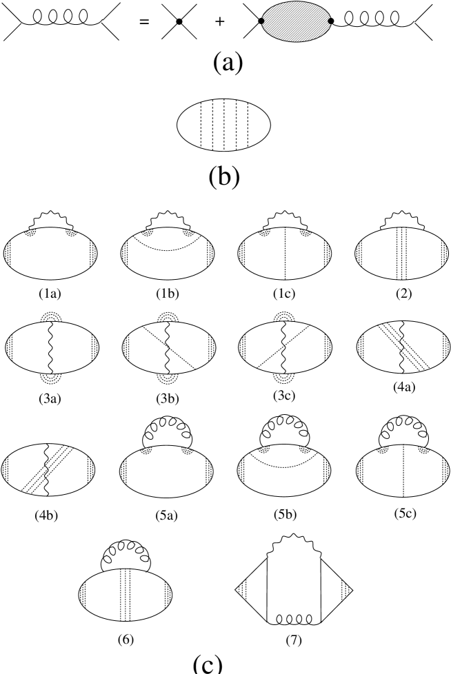
can also be obtained using the Eliashberg diagrams for ΔΔ\Delta shown in Fig. (5), or the pair propagator diagrams shown in Fig. (6).

The diagram for the first order correction to the grand potential simply consists of the β€œstring of bubbles” diagram shown in Fig. (4) Since the polarization bubbles in this diagram are just those evaluated in the previous section, we have all the information we need to derive $\Omega_{1}(\Delta)$. The only thing we need to remember is the extra symmetry factor of $1/n$ required for the diagram with $n$ bubbles. So whereas previously the RPA equation involved the series

V=V0+V0​Π​V0+V0​Π​V0​Π​V0+…=(V0βˆ’1βˆ’Ξ )βˆ’1,𝑉subscript𝑉0subscript𝑉0Ξ subscript𝑉0subscript𝑉0Ξ subscript𝑉0Ξ subscript𝑉0…superscriptsuperscriptsubscript𝑉01Ξ 1V=V_{0}+V_{0}\Pi V_{0}+V_{0}\Pi V_{0}\Pi V_{0}+\dots=(V_{0}^{-1}-\Pi)^{-1}, (44)

it now becomes

Ξ©1=V0​Π+12​V0​Π​V0​Π+13​V0​Π​V0​Π​V0​Π+…=βˆ’log⁑[V0βˆ’1βˆ’Ξ ]+log⁑[V0βˆ’1].subscriptΞ©1subscript𝑉0Ξ 12subscript𝑉0Ξ subscript𝑉0Ξ 13subscript𝑉0Ξ subscript𝑉0Ξ subscript𝑉0Π…superscriptsubscript𝑉01Ξ superscriptsubscript𝑉01\Omega_{1}=V_{0}\Pi+{1\over 2}V_{0}\Pi V_{0}\Pi+{1\over 3}V_{0}\Pi V_{0}\Pi V_{0}\Pi+\dots=-\log{[V_{0}^{-1}-\Pi]}+\log{[V_{0}^{-1}]}. (45)

After summing over all the internal variables – momentum $q$, Bose Matsubara frequency $\Omega$ and the three bosonic modes – we end up with the final expression for $\Omega_{1}$,

Ξ©1=βˆ’Tβ€‹βˆ‘Ξ©βˆ‘q{log⁑(βˆ’Ξ»βˆ’1+ΠΔ​Δ​(q,Ξ©))+log⁑[(βˆ’Ξ»βˆ’1+Πϕ​ϕ​(q,Ξ©))​[(2​VC​(q))βˆ’1+Πρ​ρ​(q,Ξ©)]+Πϕ​ρ​(q,Ξ©)2]}.subscriptΞ©1𝑇subscriptΞ©subscriptπ‘žsuperscriptπœ†1subscriptΞ Ξ”Ξ”π‘žΞ©superscriptπœ†1subscriptΞ italic-Ο•italic-Ο•π‘žΞ©delimited-[]superscript2subscriptπ‘‰πΆπ‘ž1subscriptΞ πœŒπœŒπ‘žΞ©subscriptΞ italic-Ο•πœŒsuperscriptπ‘žΞ©2\Omega_{1}=-T\sum_{\Omega}\sum_{q}\left\{\log{(-\lambda^{-1}+\Pi_{\Delta\Delta}(q,\Omega))}+\log{\big{[}(-\lambda^{-1}+\Pi_{\phi\phi}(q,\Omega))[(2V_{C}(q))^{-1}+\Pi_{\rho\rho}(q,\Omega)]+\Pi_{\phi\rho}(q,\Omega)^{2}\big{]}}\right\}. (46)

To proceed we need to minimise the total grand potential,

$${\partial\over\partial\Delta}\left\{\Omega_{0}(\Delta)+\Omega_{1}(\Delta)\right\}=0.$$ (47)

The mean-field grand potential, $\Omega_{0}(\Delta)$, is given by

$$\Omega_{0}(\Delta)=N(0){\Delta^{2}\over\lambda}+T\sum_{\omega}\sum_{k}\hbox{Tr}\left[\log{(\overline{z}-\xi_{k}\tau_{3}\sigma_{0}-\overline{\Delta}\tau_{1}\sigma_{3})}\right],$$ (48)

and after taking the derivative of $\Omega_{0}(\Delta)$ with respect to $\Delta$, we see that Eqn. (47) takes the form

$${1\over\lambda}-\pi N(0)T\sum_{\omega}{1\over U}=-{1\over\Delta}{\partial\Omega_{1}\over\partial\Delta}.$$ (49)

The next step in the procedure is to evaluate $\partial\Omega_{1}(\Delta)/\partial\Delta$. From Eqn. (46) we see that $\partial/\partial\Delta$ will be acting upon the Ξ i​jsubscriptΠ𝑖𝑗\Pi_{ij} to give

βˆ’βˆ‚Ξ©1βˆ‚Ξ”=Tβ€‹βˆ‘Ξ©βˆ‘q{βˆ‚Ξ Ξ”β€‹Ξ”βˆ‚Ξ”β€‹VΔ​Δ+βˆ‚Ξ Ο•β€‹Ο•βˆ‚Ξ”β€‹VΟ•β€‹Ο•βˆ’2β€‹βˆ‚Ξ Ο•β€‹Οβˆ‚Ξ”β€‹Vϕ​ρ+βˆ‚Ξ Οβ€‹Οβˆ‚Ξ”β€‹Vρ​ρ}.subscriptΞ©1Δ𝑇subscriptΞ©subscriptπ‘žsubscriptΠΔΔΔsubscript𝑉ΔΔsubscriptΞ italic-Ο•italic-ϕΔsubscript𝑉italic-Ο•italic-Ο•2subscriptΞ italic-Ο•πœŒΞ”subscript𝑉italic-Ο•πœŒsubscriptΞ πœŒπœŒΞ”subscriptπ‘‰πœŒπœŒ-{\partial\Omega_{1}\over\partial\Delta}=T\sum_{\Omega}\sum_{q}\left\{{\partial\Pi_{\Delta\Delta}\over\partial\Delta}V_{\Delta\Delta}+{\partial\Pi_{\phi\phi}\over\partial\Delta}V_{\phi\phi}-2{\partial\Pi_{\phi\rho}\over\partial\Delta}V_{\phi\rho}+{\partial\Pi_{\rho\rho}\over\partial\Delta}V_{\rho\rho}\right\}. (50)

From Eqn. (36) we see that the $\partial/\partial\Delta$ can act either on the coherence factor or on the denominator in the expression for Ξ i​jsubscriptΠ𝑖𝑗\Pi_{ij}. Acting on the denominator gives a result proportional to the denominator squared, corresponding to the two-ladder diagrams of Fig. (5a) in the Eliashberg approach. Similarly acting on the coherence factor leads to the one-ladder diagrams of Fig. (5b). We note that the explicit evaluation of the three-ladder diagrams of Fig. (5c) will give a zero result.

The only difficulty in taking the derivatives of the polarization bubbles, Ξ i​jsubscriptΠ𝑖𝑗\Pi_{ij}, with respect to $\Delta$ is that the quantity $u(\omega)$ present in all these equations satisfies the transcendental Eqn. (22). In Appendix C we evaluate the derivatives of the Ξ i​jsubscriptΠ𝑖𝑗\Pi_{ij} to obtain the results

βˆ‚Ξ Ξ”β€‹Ξ”βˆ‚Ξ”subscriptΠΔΔΔ\displaystyle{\partial\Pi_{\Delta\Delta}\over\partial\Delta} $\displaystyle=$ $\displaystyle-2\pi N(0)T\sum_{\omega}\left\{\left[1-{\zeta\over U^{3}}\right]^{-1}\times{1\over\Delta}{u(u^{\prime}+u)\over U^{3}U^{\prime}}{1\over D_{+}}+\left(1+{uu^{\prime}-1\over UU^{\prime}}\right)\left\{{1\over U}-{\zeta\over U^{2}}\left(1+{u(u^{\prime}-u)\over UU^{\prime}}\right)\right\}{1\over D_{+}^{2}}\right\}$ (51)
βˆ‚Ξ Ο•β€‹Ο•βˆ‚Ξ”subscriptΞ italic-Ο•italic-ϕΔ\displaystyle{\partial\Pi_{\phi\phi}\over\partial\Delta} $\displaystyle=$ $\displaystyle-2\pi N(0)T\sum_{\omega}\left\{\left[1-{\zeta\over U^{3}}\right]^{-1}\times{1\over\Delta}{u(u^{\prime}-u)\over U^{3}U^{\prime}}{1\over D_{-}}+\left(1+{uu^{\prime}+1\over UU^{\prime}}\right)\left\{{1\over U}-{\zeta\over U^{2}}\left(1+{u(u^{\prime}+u)\over UU^{\prime}}\right)\right\}{1\over D_{-}^{2}}\right\}$ (52)
βˆ‚Ξ Οβ€‹Οβˆ‚Ξ”subscriptΞ πœŒπœŒΞ”\displaystyle{\partial\Pi_{\rho\rho}\over\partial\Delta} $\displaystyle=$ $\displaystyle-2\pi N(0)T\sum_{\omega}\left\{\left[1-{\zeta\over U^{3}}\right]^{-1}\times{1\over\Delta}{u(u^{\prime}-u)\over U^{3}U^{\prime}}{1\over D_{-}}-\left(1-{uu^{\prime}+1\over UU^{\prime}}\right)\left\{{1\over U}-{\zeta\over U^{2}}\left(1+{u(u^{\prime}+u)\over UU^{\prime}}\right)\right\}{1\over D_{-}^{2}}\right\}$ (53)
βˆ‚Ξ Ο•β€‹Οβˆ‚Ξ”subscriptΞ italic-Ο•πœŒΞ”\displaystyle{\partial\Pi_{\phi\rho}\over\partial\Delta} $\displaystyle=$ $\displaystyle-2\pi N(0)T\sum_{\omega}\left\{\left[1-{\zeta\over U^{3}}\right]^{-1}\times{1\over\Delta}{u(uu^{\prime}+1)\over U^{3}U^{\prime}}{1\over D_{-}}-\left({u^{\prime}-u\over UU^{\prime}}\right)\left\{{1\over U}-{\zeta\over U^{2}}\left(1+{u(u^{\prime}+u)\over UU^{\prime}}\right)\right\}{1\over D_{-}^{2}}\right\}.$ (54)

These formulas together with Eqn. (50) lead to our final result for the first order correction to the order parameter self-consistency equation:

$\displaystyle\displaystyle{1\over N(0)\lambda}-\pi T\sum_{\omega}{1\over U}={\pi\over 2}T\sum_{\omega}T\sum_{\Omega}\sum_{q}\left[1-{\zeta\over U^{3}}\right]^{-1}\times$ (55)
$\displaystyle\displaystyle\left\{\left[{1\over\Delta^{2}}{1\over D_{+}}{u(u^{\prime}+u)\over U^{3}U^{\prime}}+{1\over\Delta}{1\over D_{+}^{2}}{1\over U}\left\{1-{\zeta\over U}\left(1+{u(u^{\prime}-u)\over UU^{\prime}}\right)\right\}\left(1+{uu^{\prime}-1\over UU^{\prime}}\right)\right]V_{\Delta\Delta}(q,\Omega)\right.$ (56)
$\displaystyle\displaystyle+{1\over\Delta^{2}}{1\over D_{-}}\left[{u(u^{\prime}-u)\over U^{3}U^{\prime}}V_{\phi\phi}(q,\Omega)-{2u(uu^{\prime}+1)\over U^{3}U^{\prime}}V_{\phi\rho}(q,\Omega)+{u(u^{\prime}-u)\over U^{3}U^{\prime}}V_{\rho\rho}(q,\Omega)\right]$ (57)
$\displaystyle\displaystyle\left.+{1\over\Delta}{1\over D_{-}^{2}}\left\{1-{\zeta\over U}\left(1+{u(u^{\prime}-u)\over UU^{\prime}}\right)\right\}\left[\left(1+{uu^{\prime}+1\over UU^{\prime}}\right)V_{\phi\phi}(q,\Omega)+{2(u^{\prime}-u)\over UU^{\prime}}V_{\phi\rho}(q,\Omega)-\left(1-{uu^{\prime}+1\over UU^{\prime}}\right)V_{\rho\rho}\right]\right\}.$ (58)

The above formula is valid for all temperatures $0\leq T\leq T_{c}$, but we are usually interested in the special cases $T=0$ and $\Delta=0$ (i.e. $T=T_{c}$). In these two cases the sum over $\omega$ on the LHS can be performed analytically to yield the two simple forms

$\displaystyle\log{\left({\Delta(0)\over\Delta_{0}(0)}\right)}$ $\displaystyle=$ $\displaystyle{\pi\over 2}T\sum_{\Omega}\sum_{q}T\sum_{\omega}\dots$ (59)
$\displaystyle\log{\left({T_{c}\over T_{c0}}\right)}$ $\displaystyle=$ $\displaystyle{\pi\over 2}T\sum_{\Omega}\sum_{q}T\sum_{\omega}\dots$ (60)

Having noted the presence of the $1/q^{d-1}$ singularities in the potentials $V_{\phi\phi}$, $V_{\phi\rho}$ and $V_{\rho\rho}$, we should now see whether the terms in Eqn. (55) containing these singularities cancel out. If we go back to Eqn. (46) for the correction to the grand potential, we see that the term ${\cal{D}}$ that goes as $q^{d-1}$ is inside a logarithm. Since $q^{d-1}$ occurs as a product, we can simply take off the term $\log{(q^{d-1})}$, and upon differentiating with respect to $\Delta$ should get zero. In other words we naively expect no singular term in Eqn. (55). However this is not quite correct since to prove that the denominator ${\cal{D}}$ vanished at $q=0$ we needed to replace $\lambda^{-1}$ using the mean-field self-consistency equation, Eqn. (23). We note that although the two sides of Eqn. (23) are numerically equal in the mean-field case, their dependences on $\Delta$ differ – $\lambda^{-1}$ gives zero under $\partial/\partial\Delta$, whilst $1/U$ does not. This discrepancy then leads to the only singular term in Eqn. (55), which may be written

$$\ln{\left({\Delta\over\Delta_{0}}\right)}_{mf}={1\over 4}\pi T\sum_{\omega}{1\over\Delta^{2}U^{3}}\left[1-{\zeta\over U^{3}}\right]^{-1}T\sum_{\Omega}\sum_{q}V_{\phi\phi}(q,\Omega).$$ (61)

Since this term tends to half the pair propagator contribution to the suppression of $T_{c}$ when we let $\Delta\rightarrow 0$, we interpret it as the phase fluctuation contribution. It is singular because of the Mermin-Wagner-Hohenberg theorem[19] which tells us that we cannot have broken symmetry states in 2D systems at finite temperature. In the following we will be mainly interested in the correction to $T_{c}$ due to Coulomb interaction and so will ignore this term.

IV First Order Correction to the Transition Temperature

We can now evaluate the first order correction to the transition temperature by linearizing the order parameter self-consistency equation with respect to $\Delta$. The former can also be obtained directly from the normal state by calculating the pair propagator $L(q,\Omega)$ to first order, and looking for the instability at $q=\Omega=0$. $L$ is given by

$$L^{-1}(q,\Omega)=\lambda^{-1}+P(q,\Omega),$$ (62)

where $P(q,\Omega)$ is the pair polarization bubble. The zeroth order polarization bubble $P_{0}(q,\Omega)$ is shown in Fig. (6b) and leads to the mean-field result

$\displaystyle L_{0}^{-1}(q,\Omega)$ $\displaystyle=$ N​(0)​[log⁑(TTc​00)+Οˆβ€‹(12+12​π​T​τs+D​q2+|Ξ©|4​π​T)βˆ’Οˆβ€‹(12)]𝑁0delimited-[]𝑇subscript𝑇𝑐00πœ“1212πœ‹π‘‡subscriptπœπ‘ π·superscriptπ‘ž2Ξ©4πœ‹π‘‡πœ“12\displaystyle N(0)\left[\log{\left({T\over T_{c00}}\right)}+\psi\left({1\over 2}+{1\over 2\pi T\tau_{s}}+{Dq^{2}+|\Omega|\over 4\pi T}\right)-\psi\left({1\over 2}\right)\right] (63)
$\displaystyle=$ N​(0)​[log⁑(TTc​0)+Οˆβ€‹(12+12​π​T​τs+D​q2+|Ξ©|4​π​T)βˆ’Οˆβ€‹(12+12​π​T​τs)],𝑁0delimited-[]𝑇subscript𝑇𝑐0πœ“1212πœ‹π‘‡subscriptπœπ‘ π·superscriptπ‘ž2Ξ©4πœ‹π‘‡πœ“1212πœ‹π‘‡subscriptπœπ‘ \displaystyle N(0)\left[\log{\left({T\over T_{c0}}\right)}+\psi\left({1\over 2}+{1\over 2\pi T\tau_{s}}+{Dq^{2}+|\Omega|\over 4\pi T}\right)-\psi\left({1\over 2}+{1\over 2\pi T\tau_{s}}\right)\right], (64)

where $T_{c00}$ is the BCS transition temperature (the mean field value in the absence of magnetic impurities), and $T_{c0}$ is the mean field value for the system with magnetic impurities. A correction to the polarization operator $\delta P(0,0)$ will lead to a change in the transition temperature, which is defined as the temperature at which the denominator of $L$ becomes zero, given by

$$\log{\left({T_{c}\over T_{c0}}\right)}={\delta P(0,0)\over N(0)}.$$ (65)

If we look at Fig. (6) we see that there are 7 diagrams which contribute to the first order correction to $T_{c}$. We will set $\Delta=0$ in the order parameter result of Eqn. (55) to get the transition temperature equation, and we will be able to identify the contribution that comes from each of the $P_{i}$ diagrams. When we set $\Delta\rightarrow 0$, then Δ​uβ†’(|Ο‰|+1/Ο„s)​sgn​(Ο‰)β†’Ξ”π‘’πœ”1subscriptπœπ‘ sgnπœ”\Delta u\rightarrow(|\omega|+1/\tau_{s})\hbox{sgn}(\omega); Δ​Uβ†’|Ο‰|+1/Ο„sβ†’Ξ”π‘ˆπœ”1subscriptπœπ‘ \Delta U\rightarrow|\omega|+1/\tau_{s}; $V_{\rho\rho}\rightarrow 2V_{C}$; $V_{\Delta\Delta}$ and $V_{\phi\phi}\rightarrow-L$; Vϕ​ρ→2​Πϕ​ρ​L​VCβ†’subscript𝑉italic-Ο•πœŒ2subscriptΞ italic-Ο•πœŒπΏsubscript𝑉𝐢V_{\phi\rho}\rightarrow 2\Pi_{\phi\rho}LV_{C}. The coherence factors then become Heaviside functions that set the relative signs of the frequencies

$\displaystyle 1-{uu^{\prime}\pm 1\over UU^{\prime}}$ $\displaystyle\rightarrow$ $\displaystyle 2\theta(-\omega(\omega+\Omega))$ (66)
$\displaystyle 1+{uu^{\prime}\pm 1\over UU^{\prime}}$ $\displaystyle\rightarrow$ $\displaystyle 2\theta(\omega(\omega+\Omega)).$ (67)

The two denominators, $D_{\pm}$, both become $Dq^{2}+|\Omega|$ for $\omega$, $\omega+\Omega$ of opposite sign; D​q2+|2​ω+Ξ©|+2/Ο„s𝐷superscriptπ‘ž22πœ”Ξ©2subscriptπœπ‘ Dq^{2}+|2\omega+\Omega|+2/\tau_{s} for $\omega$, $\omega+\Omega$ of the same sign. Making all these substitutions leads to

$\displaystyle P_{1}$ $\displaystyle=$ βˆ’Ο€β€‹N​(0)​Tβ€‹βˆ‘Ο‰Tβ€‹βˆ‘Ξ©βˆ‘q[1(|Ο‰|+1/Ο„s)2​1(D​q2+|Ξ©|)+2(|Ο‰|+1/Ο„s)​1(D​q2+|Ξ©|)2]​VC​(q,Ξ©)​θ​(βˆ’Ο‰β€‹(Ο‰+Ξ©))πœ‹π‘0𝑇subscriptπœ”π‘‡subscriptΞ©subscriptπ‘ždelimited-[]1superscriptπœ”1subscriptπœπ‘ 21𝐷superscriptπ‘ž2Ξ©2πœ”1subscriptπœπ‘ 1superscript𝐷superscriptπ‘ž2Ξ©2subscriptπ‘‰πΆπ‘žΞ©πœƒπœ”πœ”Ξ©\displaystyle-\pi N(0)T\sum_{\omega}T\sum_{\Omega}\sum_{q}\left[{1\over(|\omega|+1/\tau_{s})^{2}}{1\over(Dq^{2}+|\Omega|)}+{2\over(|\omega|+1/\tau_{s})}{1\over(Dq^{2}+|\Omega|)^{2}}\right]V_{C}(q,\Omega)\theta(-\omega(\omega+\Omega)) (68)
$\displaystyle P_{2}$ $\displaystyle=$ π​N​(0)​Tβ€‹βˆ‘Ο‰Tβ€‹βˆ‘Ξ©βˆ‘q1(|Ο‰|+1/Ο„s)2​1D​q2+|2​ω+Ξ©|+2/Ο„s​VC​(q,Ξ©)​θ​(ω​(Ο‰+Ξ©))πœ‹π‘0𝑇subscriptπœ”π‘‡subscriptΞ©subscriptπ‘ž1superscriptπœ”1subscriptπœπ‘ 21𝐷superscriptπ‘ž22πœ”Ξ©2subscriptπœπ‘ subscriptπ‘‰πΆπ‘žΞ©πœƒπœ”πœ”Ξ©\displaystyle\pi N(0)T\sum_{\omega}T\sum_{\Omega}\sum_{q}{1\over(|\omega|+1/\tau_{s})^{2}}{1\over Dq^{2}+|2\omega+\Omega|+2/\tau_{s}}V_{C}(q,\Omega)\theta(\omega(\omega+\Omega)) (69)
$\displaystyle P_{3}$ $\displaystyle=$ βˆ’Ο€β€‹N​(0)​Tβ€‹βˆ‘Ο‰Tβ€‹βˆ‘Ξ©βˆ‘q1(|Ο‰|+1/Ο„s)​(|Ο‰+Ξ©|+1/Ο„s)​[1(D​q2+|Ξ©|)+2/Ο„s(D​q2+|Ξ©|)2]​VC​(q,Ξ©)​θ​(βˆ’Ο‰β€‹(Ο‰+Ξ©))πœ‹π‘0𝑇subscriptπœ”π‘‡subscriptΞ©subscriptπ‘ž1πœ”1subscriptπœπ‘ πœ”Ξ©1subscriptπœπ‘ delimited-[]1𝐷superscriptπ‘ž2Ξ©2subscriptπœπ‘ superscript𝐷superscriptπ‘ž2Ξ©2subscriptπ‘‰πΆπ‘žΞ©πœƒπœ”πœ”Ξ©\displaystyle-\pi N(0)T\sum_{\omega}T\sum_{\Omega}\sum_{q}{1\over(|\omega|+1/\tau_{s})(|\omega+\Omega|+1/\tau_{s})}\left[{1\over(Dq^{2}+|\Omega|)}+{2/\tau_{s}\over(Dq^{2}+|\Omega|)^{2}}\right]V_{C}(q,\Omega)\theta(-\omega(\omega+\Omega)) (70)
$\displaystyle P_{4}$ $\displaystyle=$ βˆ’Ο€β€‹N​(0)​Tβ€‹βˆ‘Ο‰Tβ€‹βˆ‘Ξ©βˆ‘q1(|Ο‰|+1/Ο„s)​(|Ο‰+Ξ©|+1/Ο„s)​1(D​q2+|2​ω+Ξ©|+2/Ο„s)​VC​(q,Ξ©)​θ​(ω​(Ο‰+Ξ©))πœ‹π‘0𝑇subscriptπœ”π‘‡subscriptΞ©subscriptπ‘ž1πœ”1subscriptπœπ‘ πœ”Ξ©1subscriptπœπ‘ 1𝐷superscriptπ‘ž22πœ”Ξ©2subscriptπœπ‘ subscriptπ‘‰πΆπ‘žΞ©πœƒπœ”πœ”Ξ©\displaystyle-\pi N(0)T\sum_{\omega}T\sum_{\Omega}\sum_{q}{1\over(|\omega|+1/\tau_{s})(|\omega+\Omega|+1/\tau_{s})}{1\over(Dq^{2}+|2\omega+\Omega|+2/\tau_{s})}V_{C}(q,\Omega)\theta(\omega(\omega+\Omega)) (71)
$\displaystyle P_{5}$ $\displaystyle=$ βˆ’Ο€β€‹N​(0)​Tβ€‹βˆ‘Ο‰Tβ€‹βˆ‘Ξ©βˆ‘q1(|Ο‰|+1/Ο„s)2​[1(D​q2+|2​ω+Ξ©|+2/Ο„s)+|Ο‰|βˆ’1/Ο„s(D​q2+|2​ω+Ξ©|+2/Ο„s)2]​L​(q,Ξ©)​θ​(ω​(Ο‰+Ξ©))πœ‹π‘0𝑇subscriptπœ”π‘‡subscriptΞ©subscriptπ‘ž1superscriptπœ”1subscriptπœπ‘ 2delimited-[]1𝐷superscriptπ‘ž22πœ”Ξ©2subscriptπœπ‘ πœ”1subscriptπœπ‘ superscript𝐷superscriptπ‘ž22πœ”Ξ©2subscriptπœπ‘ 2πΏπ‘žΞ©πœƒπœ”πœ”Ξ©\displaystyle-\pi N(0)T\sum_{\omega}T\sum_{\Omega}\sum_{q}{1\over(|\omega|+1/\tau_{s})^{2}}\left[{1\over(Dq^{2}+|2\omega+\Omega|+2/\tau_{s})}+{|\omega|-1/\tau_{s}\over(Dq^{2}+|2\omega+\Omega|+2/\tau_{s})^{2}}\right]L(q,\Omega)\theta(\omega(\omega+\Omega)) (72)
$\displaystyle P_{6}$ $\displaystyle=$ π​N​(0)​Tβ€‹βˆ‘Ο‰Tβ€‹βˆ‘Ξ©βˆ‘q1(|Ο‰|+1/Ο„s)2​(D​q2+|Ξ©|)​L​(q,Ξ©)​θ​(βˆ’Ο‰β€‹(Ο‰+Ξ©))πœ‹π‘0𝑇subscriptπœ”π‘‡subscriptΞ©subscriptπ‘ž1superscriptπœ”1subscriptπœπ‘ 2𝐷superscriptπ‘ž2Ξ©πΏπ‘žΞ©πœƒπœ”πœ”Ξ©\displaystyle\pi N(0)T\sum_{\omega}T\sum_{\Omega}\sum_{q}{1\over(|\omega|+1/\tau_{s})^{2}(Dq^{2}+|\Omega|)}L(q,\Omega)\theta(-\omega(\omega+\Omega)) (73)
$\displaystyle P_{7}$ $\displaystyle=$ $\displaystyle 4\pi^{2}N(0)^{2}T\sum_{\Omega}\sum_{q}\left[T\sum_{\omega}{\hbox{sgn}(\omega+\Omega)\over(|\omega|+1/\tau_{s})(Dq^{2}+|\omega|+|\omega+\Omega|+2/\tau_{s})\theta(\omega(\omega+\Omega)))}\right]^{2}V_{C}(q,\Omega)L(q,\Omega).$ (74)

The assignment of terms to the polarization bubble diagram they would arise from if we had done the calculation by that method is unique, and can be summarised below:

  • $P_{1}$ : term proportional to $V_{C}$, $\theta(-\omega(\omega+\Omega))$ with no |Ο‰+Ξ©|+1/Ο„sπœ”Ξ©1subscriptπœπ‘ |\omega+\Omega|+1/\tau_{s} denominator.

  • $P_{2}$ : term proportional to $V_{C}$, $\theta(\omega(\omega+\Omega))$ with no |Ο‰+Ξ©|+1/Ο„sπœ”Ξ©1subscriptπœπ‘ |\omega+\Omega|+1/\tau_{s} denominator.

  • $P_{3}$ : term proportional to $V_{C}$, $\theta(-\omega(\omega+\Omega))$ with |Ο‰+Ξ©|+1/Ο„sπœ”Ξ©1subscriptπœπ‘ |\omega+\Omega|+1/\tau_{s} denominator.

  • $P_{4}$ : term proportional to $V_{C}$, $\theta(\omega(\omega+\Omega))$ with no |Ο‰+Ξ©|+1/Ο„sπœ”Ξ©1subscriptπœπ‘ |\omega+\Omega|+1/\tau_{s} denominator.

  • $P_{5}$ : term proportional to $L$ and $\theta(-\omega(\omega+\Omega))$.

  • $P_{6}$ : term proportional to $L$ and $\theta(\omega(\omega+\Omega))$.

  • $P_{7}$ : term proportional to $LV_{C}$.

We find that these reduce to the results of I when we set 1/Ο„sβ†’0β†’1subscriptπœπ‘ 01/\tau_{s}\rightarrow 0, providing a useful consistency check on the present calculation.

To evaluate the correction to $T_{c}$ we split it into two parts: the Coulomb part consisting of those parts that contain a Coulomb propagator, ($P_{1}-P_{4}$, $P_{7}$), and consequently require special attention at $q=0$, and the fluctuation part consisting of those terms that contain only a fluctuation propagator, ($P_{5}$, $P_{6}$). Performing the $\omega$-sum first we get for the Coulomb part

$\displaystyle\log{\left({T_{c}\over T_{c0}}\right)}=-T_{c}\sum_{\Omega}\sum_{q}\left\{{1\over 2\pi T_{c}}{Dq^{2}\over\Omega^{2}-(Dq^{2})^{2}}\psi^{\prime}\left({1\over 2}+{1\over 2\pi T_{c}\tau_{s}}+{|\Omega|\over 2\pi T_{c}}\right)\right.$ (75)
$\displaystyle+$ [2​D​q2​[Ξ©2+(D​q2)2]|Ξ©|​[Ξ©2βˆ’(D​q2)2]2βˆ’(2Ο„s)​D​q2|Ξ©|​(|Ξ©|+2Ο„s)​(|Ξ©|+D​q2)]​[Οˆβ€‹(12+12​π​Tc​τs+|Ξ©|2​π​Tc)βˆ’Οˆβ€‹(12+12​π​Tc​τs)]delimited-[]2𝐷superscriptπ‘ž2delimited-[]superscriptΞ©2superscript𝐷superscriptπ‘ž22Ξ©superscriptdelimited-[]superscriptΞ©2superscript𝐷superscriptπ‘ž2222subscriptπœπ‘ π·superscriptπ‘ž2ΩΩ2subscriptπœπ‘ Ξ©π·superscriptπ‘ž2delimited-[]πœ“1212πœ‹subscript𝑇𝑐subscriptπœπ‘ Ξ©2πœ‹subscriptπ‘‡π‘πœ“1212πœ‹subscript𝑇𝑐subscriptπœπ‘ \displaystyle\left.\left[{2Dq^{2}[\Omega^{2}+(Dq^{2})^{2}]\over|\Omega|[\Omega^{2}-(Dq^{2})^{2}]^{2}}-{\displaystyle\left({2\over\tau_{s}}\right)Dq^{2}\over\displaystyle|\Omega|\left(|\Omega|+{2\over\tau_{s}}\right)\left(|\Omega|+Dq^{2}\right)}\right]\left[\psi\left({1\over 2}+{1\over 2\pi T_{c}\tau_{s}}+{|\Omega|\over 2\pi T_{c}}\right)-\psi\left({1\over 2}+{1\over 2\pi T_{c}\tau_{s}}\right)\right]\right. (76)
$\displaystyle-$ $\displaystyle\left.\displaystyle{4(Dq^{2})^{2}\over[\Omega^{2}-(Dq^{2})^{2}]^{2}}{\displaystyle\left[\psi\left({1\over 2}+{1\over 2\pi T_{c}\tau_{s}}+{|\Omega|\over 2\pi T_{c}}\right)-\psi\left({1\over 2}+{1\over 2\pi T_{c}\tau_{s}}\right)\right]^{2}\over\displaystyle\left[\psi\left({1\over 2}+{1\over 2\pi T_{c}\tau_{s}}+{Dq^{2}+|\Omega|)\over 4\pi T_{c}}\right)-\psi\left({1\over 2}+{1\over 2\pi T_{c}\tau_{s}}\right)\right]}\right\}V_{C}(q,\Omega).$ (77)

Since the worst singularity possible in $V_{C}(q,\Omega)$ at $q=0$ goes as $1/q^{2}$, the overall $q^{2}$ factor multiplying $V_{C}$ in the above expression means that this singularity is removed. It follows that the removal of the $q=0$ singularity in the Coulomb part is unaffected by the addition of magnetic impurities – this is because it is a general feature enforced by gauge invariance, as we will show in Appendix B.

To calculate the Coulombic suppression term of Eqn. (75), we change variables to $m=\Omega/2\pi T$ and $y=Dq^{2}/2\pi T$, noting that $\sum_{q}=\int dy/(8\pi^{2}DT)$, and

$$N(0)V_{C}(q,\Omega)=N(0)\left[{q^{2}\over 4\pi e^{2}}+{2N(0)Dq^{2}\over Dq^{2}+|\Omega|}\right]^{-1}\approx{Dq^{2}+|\Omega|\over 2Dq^{2}}={m+y\over 2y}.$$ (78)

This leads to the result

$\displaystyle\log{\left({T_{c}\over T_{c0}}\right)}=\displaystyle-{1\over 8\pi^{2}N(0)D}\sum_{m=1}^{M}\int_{0}^{M}dy$ $\displaystyle\left\{{1\over m-y}\psi^{\prime}\left({1\over 2}+\alpha\right)\right.$ (79)
$\displaystyle+$ $\displaystyle\left[{2y(m^{2}+y^{2})\over m(m^{2}-y^{2})^{2}}-{2\alpha y\over m(m+2\alpha)(m+y)}\right]\left[\psi\left({1\over 2}+\alpha+m\right)-\psi\left({1\over 2}+\alpha\right)\right]$ (80)
$\displaystyle-$ $\displaystyle\left.{4y\over(m-y)(m^{2}-y^{2})}{\left[\psi\left({1\over 2}+\alpha+m\right)-\left({1\over 2}+\alpha\right)\right]^{2}\over\left[\psi\left({1\over 2}+\alpha+{m+y\over 2}\right)-\psi\left({1\over 2}+\alpha\right)\right]}\right\},$ (81)

where Ξ±=1/2​π​Tc​τs𝛼12πœ‹subscript𝑇𝑐subscriptπœπ‘ \alpha=1/2\pi T_{c}\tau_{s} and the upper cutoff $M=1/2\pi T_{c}\tau$. The leading order term is that which goes like $1/y$ at large $y$, leading to logarithmic behavior. To isolate this, we add and subtract the term

$\displaystyle\sum_{m=1}^{M}\int_{0}^{M}{dy\over(m+y)}\left\{\left({2\over m}-{2\alpha\over m(m+2\alpha)}\right)\left[\psi\left({1\over 2}+\alpha+m\right)-\psi\left({1\over 2}+\alpha\right)\right]-\psi^{\prime}\left({1\over 2}+\alpha\right)\right\}$ (82)
$\displaystyle=$ $\displaystyle\sum_{m=1}^{M}\ln{\left({M+m\over m}\right)}\left\{{2(m+\alpha)\over m(m+2\alpha)}\left[\psi\left({1\over 2}+\alpha+m\right)-\psi\left({1\over 2}+\alpha\right)\right]-\psi^{\prime}\left({1\over 2}+\alpha\right)\right\},$ (83)

to give the result

$\displaystyle\ln{\left({T_{c}\over T_{c0}}\right)}=$ $\displaystyle-$ RΒ Β Β Β R0{βˆ‘m=1Mln(M+mm)[2​(m+Ξ±)m​(m+2​α)[ψ(12+Ξ±+m)βˆ’Οˆ(12+Ξ±)]βˆ’Οˆβ€²(12+Ξ±)]\displaystyle{R_{\mathchoice{\vbox{\vbox{\hrule height=0.4pt\hbox{\vrule width=0.4pt,height=3.0pt\kern 3.0pt\vrule width=0.4pt} \hrule height=0.4pt}}}{\vbox{\vbox{\hrule height=0.4pt\hbox{\vrule width=0.4pt,height=3.0pt\kern 3.0pt\vrule width=0.4pt} \hrule height=0.4pt}}}{\vbox{\vbox{\hrule height=0.3pt\hbox{\vrule width=0.3pt,height=2.1pt\kern 2.1pt\vrule width=0.3pt} \hrule height=0.3pt}}}{\vbox{\vbox{\hrule height=0.3pt\hbox{\vrule width=0.3pt,height=1.5pt\kern 1.5pt\vrule width=0.3pt} \hrule height=0.3pt}}}}\over R_{0}}\left\{\sum_{m=1}^{M}\ln{\left({M+m\over m}\right)}\left[{2(m+\alpha)\over m(m+2\alpha)}\left[\psi\left({1\over 2}+\alpha+m\right)-\psi\left({1\over 2}+\alpha\right)\right]-\psi^{\prime}\left({1\over 2}+\alpha\right)\right]\right. (84)
$\displaystyle-$ $\displaystyle\sum_{m=1}^{M}\int_{0}^{M}dy{4y\over(m-y)(m^{2}-y^{2})}\left[{\left[\psi\left({1\over 2}+\alpha+m\right)-\psi\left({1\over 2}+\alpha\right)\right]^{2}\over\left[\psi\left({1\over 2}+\alpha+{m+y\over 2}\right)\right]}\right.$ (85)
$\displaystyle-$ $\displaystyle\left.\left.\left[\psi\left({1\over 2}+\alpha+m\right)-\psi\left({1\over 2}+\alpha\right)\right]+{y-m\over 2}\psi^{\prime}\left({1\over 2}+\alpha\right)\right]\right\},$ (86)

where we have noted that 1/8​π2​N​(0)​D=RΒ Β Β Β Β /R018superscriptπœ‹2𝑁0𝐷subscript𝑅     subscript𝑅01/8\pi^{2}N(0)D=R_{\mathchoice{\vbox{\vbox{\hrule height=0.4pt\hbox{\vrule width=0.4pt,height=3.0pt\kern 3.0pt\vrule width=0.4pt} \hrule height=0.4pt}}}{\vbox{\vbox{\hrule height=0.4pt\hbox{\vrule width=0.4pt,height=3.0pt\kern 3.0pt\vrule width=0.4pt} \hrule height=0.4pt}}}{\vbox{\vbox{\hrule height=0.3pt\hbox{\vrule width=0.3pt,height=2.1pt\kern 2.1pt\vrule width=0.3pt} \hrule height=0.3pt}}}{\vbox{\vbox{\hrule height=0.3pt\hbox{\vrule width=0.3pt,height=1.5pt\kern 1.5pt\vrule width=0.3pt} \hrule height=0.3pt}}}}/R_{0}. We could now proceed to evaluate this expression, but before we do so, let us consider the domain of validity of the first-order perturbative result.

V Beyond Perturbation Theory

Since we now have the full first-order perturbative correction to the transition temperature due to the effect of disorder on the Coulomb interaction, we could in principle plot curves of Tc​(RΒ Β Β Β Β ,1/Ο„s)subscript𝑇𝑐subscript𝑅     1subscriptπœπ‘ T_{c}(R_{\mathchoice{\vbox{\vbox{\hrule height=0.4pt\hbox{\vrule width=0.4pt,height=3.0pt\kern 3.0pt\vrule width=0.4pt} \hrule height=0.4pt}}}{\vbox{\vbox{\hrule height=0.4pt\hbox{\vrule width=0.4pt,height=3.0pt\kern 3.0pt\vrule width=0.4pt} \hrule height=0.4pt}}}{\vbox{\vbox{\hrule height=0.3pt\hbox{\vrule width=0.3pt,height=2.1pt\kern 2.1pt\vrule width=0.3pt} \hrule height=0.3pt}}}{\vbox{\vbox{\hrule height=0.3pt\hbox{\vrule width=0.3pt,height=1.5pt\kern 1.5pt\vrule width=0.3pt} \hrule height=0.3pt}}}},1/\tau_{s}) and compare to experiment. However the curves of $T_{c}$ vs RΒ Β Β Β Β subscript𝑅     R_{\mathchoice{\vbox{\vbox{\hrule height=0.4pt\hbox{\vrule width=0.4pt,height=3.0pt\kern 3.0pt\vrule width=0.4pt} \hrule height=0.4pt}}}{\vbox{\vbox{\hrule height=0.4pt\hbox{\vrule width=0.4pt,height=3.0pt\kern 3.0pt\vrule width=0.4pt} \hrule height=0.4pt}}}{\vbox{\vbox{\hrule height=0.3pt\hbox{\vrule width=0.3pt,height=2.1pt\kern 2.1pt\vrule width=0.3pt} \hrule height=0.3pt}}}{\vbox{\vbox{\hrule height=0.3pt\hbox{\vrule width=0.3pt,height=1.5pt\kern 1.5pt\vrule width=0.3pt} \hrule height=0.3pt}}}} for different values of 1/Ο„s1subscriptπœπ‘ 1/\tau_{s} would simply be exponential decays with different initial slopes. First-order perturbation theory is unable to treat the strong disorder region, and so cannot lead to the complete destruction of the superconductivity by non-magnetic disorder. If we are to consider the effects of arbitrary disorder strength, we must work beyond perturbation theory. In what follows we discuss two methods of doing this, and compare the results we obtain from them.

The simplest way to proceed is to β€œself-consistently” solve the first-order perturbative expression of Eq. (84). This simply means that we replace $T_{c0}$ by $T_{c}$ on the right-hand side of Eq. (84), and solve the implicit equation we obtain for $T_{c}$ which has the form

ln⁑(TcTc​0)=Οˆβ€‹(12)βˆ’Οˆβ€‹(12+12​π​Tc​τs)βˆ’RΒ Β Β Β Β R0​f​(Tc,1/Ο„s).subscript𝑇𝑐subscript𝑇𝑐0πœ“12πœ“1212πœ‹subscript𝑇𝑐subscriptπœπ‘ subscript𝑅     subscript𝑅0𝑓subscript𝑇𝑐1subscriptπœπ‘ \ln{\left({T_{c}\over T_{c0}}\right)}=\psi\left({1\over 2}\right)-\psi\left({1\over 2}+{1\over 2\pi T_{c}\tau_{s}}\right)-{R_{\mathchoice{\vbox{\vbox{\hrule height=0.4pt\hbox{\vrule width=0.4pt,height=3.0pt\kern 3.0pt\vrule width=0.4pt} \hrule height=0.4pt}}}{\vbox{\vbox{\hrule height=0.4pt\hbox{\vrule width=0.4pt,height=3.0pt\kern 3.0pt\vrule width=0.4pt} \hrule height=0.4pt}}}{\vbox{\vbox{\hrule height=0.3pt\hbox{\vrule width=0.3pt,height=2.1pt\kern 2.1pt\vrule width=0.3pt} \hrule height=0.3pt}}}{\vbox{\vbox{\hrule height=0.3pt\hbox{\vrule width=0.3pt,height=1.5pt\kern 1.5pt\vrule width=0.3pt} \hrule height=0.3pt}}}}\over R_{0}}f(T_{c},1/\tau_{s}). (87)

Here f​(Tc,1/Ο„s)𝑓subscript𝑇𝑐1subscriptπœπ‘ f(T_{c},1/\tau_{s}) is the complicated expression on the right-hand side of Eq. (84), whilst the first term is just the mean-field suppression of $T_{c}$ by the magnetic impurities. From our knowledge of the situation without magnetic impurities, we know that unphysical re-entrance problems may arise with the solution of this equation, and we should not take it too seriously in the region where superconductivity is strongly suppressed.

The fact that we cannot trust the results obtained from this β€œself-consistent” theory leads us to ask the question of how to correctly go beyond first-order perturbation theory. The best approach is to derive the effective field theory from which the perturbation series may be deduced – in this case a non-linear sigma model[20] – and treat this using the renormalization group. This has been done by Finkel’stein[10] for the system without magnetic impurities, but has the problem that it is very difficult, and would become even more so if magnetic impurities were added. Recently Oreg and Finkel’stein[12] demonstrated that the same results could be obtained using a much simpler non-perturbative resummation technique, which we show diagrammatically in Fig. (7). The method uses a featureless Coulomb interaction of magnitude $N(0)V_{C}=1/2$, consistent with the cancellation of the $1/q^{d-1}$ divergence discussed earlier, and keeps only diagrams 3 and 4 of Fig. (6), since they give the greatest contribution. This leads to the equation for the pair scattering amplitude, $\Gamma(\omega_{n},\omega_{l})$,

Γ​(Ο‰n,Ο‰l)=βˆ’|Ξ»|+t​Λ​(Ο‰n,Ο‰l)βˆ’Ο€β€‹Tβ€‹βˆ‘m=βˆ’(M+1)M[βˆ’|Ξ»|+t​Λ​(Ο‰n,Ο‰m)]​1|Ο‰m|+1/Ο„s​Γ​(Ο‰m,Ο‰l),Ξ“subscriptπœ”π‘›subscriptπœ”π‘™πœ†π‘‘Ξ›subscriptπœ”π‘›subscriptπœ”π‘™πœ‹π‘‡superscriptsubscriptπ‘šπ‘€1𝑀delimited-[]πœ†π‘‘Ξ›subscriptπœ”π‘›subscriptπœ”π‘š1subscriptπœ”π‘š1subscriptπœπ‘ Ξ“subscriptπœ”π‘šsubscriptπœ”π‘™\Gamma(\omega_{n},\omega_{l})=-|\lambda|+t\Lambda(\omega_{n},\omega_{l})-\pi T\sum_{m=-(M+1)}^{M}[-|\lambda|+t\Lambda(\omega_{n},\omega_{m})]{1\over|\omega_{m}|+1/\tau_{s}}\Gamma(\omega_{m},\omega_{l}), (88)

where $\omega_{n}=2\pi T(n+1/2)$ is a Fermi Matsubara frequency, and the upper cut-off $M=1/2\pi T\tau$. The amplitude $\Lambda(\omega_{n},\omega_{l})$ is given by

Λ​(Ο‰n,Ο‰l)={ln⁑[1(|Ο‰n|+|Ο‰l|)​τ]Ο‰n​ωl<0ln⁑[1(|Ο‰n|+|Ο‰l|+2/Ο„s)​τ]Ο‰n​ωl>0Ξ›subscriptπœ”π‘›subscriptπœ”π‘™cases1subscriptπœ”π‘›subscriptπœ”π‘™πœsubscriptπœ”π‘›subscriptπœ”π‘™01subscriptπœ”π‘›subscriptπœ”π‘™2subscriptπœπ‘ πœsubscriptπœ”π‘›subscriptπœ”π‘™0\Lambda(\omega_{n},\omega_{l})=\cases{\displaystyle\ln{\left[{1\over(|\omega_{n}|+|\omega_{l}|)\tau}\right]}&$\quad\omega_{n}\omega_{l}<0$\cr\displaystyle\ln{\left[{1\over(|\omega_{n}|+|\omega_{l}|+2/\tau_{s})\tau}\right]}&$\quad\omega_{n}\omega_{l}>0$\cr} (89)

where the breaking of time-reversal invariance by the spin-flip scattering means that $\Lambda$ has a different form depending upon the relative signs of its two Matsubara frequencies. If we treat the $\Gamma(\omega_{n},\omega_{m})$ as elements of a matrix $\hat{\Gamma}$, the matrix equation for $\hat{\Gamma}$ can be solved to yield

Ξ“^=Ο‰^1/2​(I^βˆ’|Ξ»|​Π^)βˆ’1​ω^βˆ’1/2​(βˆ’|Ξ»|​1^+t​Λ^),^Ξ“superscript^πœ”12superscript^πΌπœ†^Ξ 1superscript^πœ”12πœ†^1𝑑^Ξ›\hat{\Gamma}=\hat{\omega}^{1/2}(\hat{I}-|\lambda|\hat{\Pi})^{-1}\hat{\omega}^{-1/2}(-|\lambda|\hat{1}+t\hat{\Lambda}), (90)

where

Ξ ^=12​ω^βˆ’1/2​[1^βˆ’|Ξ»|βˆ’1​t​Λ^]​ω^βˆ’1/2,^Ξ 12superscript^πœ”12delimited-[]^1superscriptπœ†1𝑑^Ξ›superscript^πœ”12\hat{\Pi}={1\over 2}\hat{\omega}^{-1/2}[\hat{1}-|\lambda|^{-1}t\hat{\Lambda}]\hat{\omega}^{-1/2}, (91)

$\hat{\omega}_{nm}=(n+1/2+\alpha)\delta_{nm}$, $\hat{\Lambda}_{nm}=\Lambda(\omega_{n},\omega_{m})$, $\hat{1}_{nm}=1$ and $\hat{I}_{nm}=\delta_{nm}$. The matrix $\hat{\Gamma}$ becomes singular when an eigenvalue of Ξ ^^Ξ \hat{\Pi} equals $1/|\lambda|$, and this signals the onset of superconductivity. Note that the matrix Ξ ^^Ξ \hat{\Pi} depends on temperature both through the temperature dependence of its elements, and also through its rank $2M$. To find $T_{c}$, we start at the BCS value $T_{c0}$, which corresponds to a value of $M$ given by $M_{0}=1/2\pi T_{c0}\tau$. We decrease the temperature $T$ by increasing the upper cut-off $M$ successively by one. For each value of $M$, we construct the matrix Ξ ^^Ξ \hat{\Pi}, and diagonalise it. When its lowest eigenvalue equals $1/|\lambda|$, we have reached the transition temperature $T_{c}$, which is given by $T_{c}/T_{c0}=M_{0}/M$. This method allows us to go to as low a temperature as we like, provided that we are prepared to diagonalize large enough matrices.

We will now plot curves of $T_{c}$ vs RΒ Β Β Β Β subscript𝑅     R_{\mathchoice{\vbox{\vbox{\hrule height=0.4pt\hbox{\vrule width=0.4pt,height=3.0pt\kern 3.0pt\vrule width=0.4pt} \hrule height=0.4pt}}}{\vbox{\vbox{\hrule height=0.4pt\hbox{\vrule width=0.4pt,height=3.0pt\kern 3.0pt\vrule width=0.4pt} \hrule height=0.4pt}}}{\vbox{\vbox{\hrule height=0.3pt\hbox{\vrule width=0.3pt,height=2.1pt\kern 2.1pt\vrule width=0.3pt} \hrule height=0.3pt}}}{\vbox{\vbox{\hrule height=0.3pt\hbox{\vrule width=0.3pt,height=1.5pt\kern 1.5pt\vrule width=0.3pt} \hrule height=0.3pt}}}} for fixed 1/Ο„s1subscriptπœπ‘ 1/\tau_{s}, and $T_{c}$ vs 1/Ο„s1subscriptπœπ‘ 1/\tau_{s} for fixed RΒ Β Β Β Β subscript𝑅     R_{\mathchoice{\vbox{\vbox{\hrule height=0.4pt\hbox{\vrule width=0.4pt,height=3.0pt\kern 3.0pt\vrule width=0.4pt} \hrule height=0.4pt}}}{\vbox{\vbox{\hrule height=0.4pt\hbox{\vrule width=0.4pt,height=3.0pt\kern 3.0pt\vrule width=0.4pt} \hrule height=0.4pt}}}{\vbox{\vbox{\hrule height=0.3pt\hbox{\vrule width=0.3pt,height=2.1pt\kern 2.1pt\vrule width=0.3pt} \hrule height=0.3pt}}}{\vbox{\vbox{\hrule height=0.3pt\hbox{\vrule width=0.3pt,height=1.5pt\kern 1.5pt\vrule width=0.3pt} \hrule height=0.3pt}}}}, derived both from the self-consistent perturbation theory of Eqn. (87), and from the non-perturbative resummation approach of Eqn. (88). This is done in Fig.Β (8), and we see that the two approaches are in rough agreement. The resummation technique is seen to remove the re-entrance problem which occurs in the $\alpha=0$ curve at large RΒ Β Β Β Β subscript𝑅     R_{\mathchoice{\vbox{\vbox{\hrule height=0.4pt\hbox{\vrule width=0.4pt,height=3.0pt\kern 3.0pt\vrule width=0.4pt} \hrule height=0.4pt}}}{\vbox{\vbox{\hrule height=0.4pt\hbox{\vrule width=0.4pt,height=3.0pt\kern 3.0pt\vrule width=0.4pt} \hrule height=0.4pt}}}{\vbox{\vbox{\hrule height=0.3pt\hbox{\vrule width=0.3pt,height=2.1pt\kern 2.1pt\vrule width=0.3pt} \hrule height=0.3pt}}}{\vbox{\vbox{\hrule height=0.3pt\hbox{\vrule width=0.3pt,height=1.5pt\kern 1.5pt\vrule width=0.3pt} \hrule height=0.3pt}}}}, but surprisingly this re-entrance seems to be partially cured by the presence of magnetic impurities.

The above curves are fine from the theorist’s point of view, but experimentally what is measured is the suppression of $T_{c}$ by a certain fixed amount of magnetic impurities as the thickness of the superconductor is altered. The data is then presented in the form of the pair-breaking per magnetic impurity which can be written as

α′​(RΒ Β Β Β Β )=Tc​(RΒ Β Β Β Β ,0)βˆ’Tc​(RΒ Β Β Β Β ,1/Ο„s)1/Ο„s,superscript𝛼′subscript𝑅     subscript𝑇𝑐subscript𝑅     0subscript𝑇𝑐subscript𝑅     1subscriptπœπ‘ 1subscriptπœπ‘ \alpha^{\prime}(R_{\mathchoice{\vbox{\vbox{\hrule height=0.4pt\hbox{\vrule width=0.4pt,height=3.0pt\kern 3.0pt\vrule width=0.4pt} \hrule height=0.4pt}}}{\vbox{\vbox{\hrule height=0.4pt\hbox{\vrule width=0.4pt,height=3.0pt\kern 3.0pt\vrule width=0.4pt} \hrule height=0.4pt}}}{\vbox{\vbox{\hrule height=0.3pt\hbox{\vrule width=0.3pt,height=2.1pt\kern 2.1pt\vrule width=0.3pt} \hrule height=0.3pt}}}{\vbox{\vbox{\hrule height=0.3pt\hbox{\vrule width=0.3pt,height=1.5pt\kern 1.5pt\vrule width=0.3pt} \hrule height=0.3pt}}}})={T_{c}(R_{\mathchoice{\vbox{\vbox{\hrule height=0.4pt\hbox{\vrule width=0.4pt,height=3.0pt\kern 3.0pt\vrule width=0.4pt} \hrule height=0.4pt}}}{\vbox{\vbox{\hrule height=0.4pt\hbox{\vrule width=0.4pt,height=3.0pt\kern 3.0pt\vrule width=0.4pt} \hrule height=0.4pt}}}{\vbox{\vbox{\hrule height=0.3pt\hbox{\vrule width=0.3pt,height=2.1pt\kern 2.1pt\vrule width=0.3pt} \hrule height=0.3pt}}}{\vbox{\vbox{\hrule height=0.3pt\hbox{\vrule width=0.3pt,height=1.5pt\kern 1.5pt\vrule width=0.3pt} \hrule height=0.3pt}}}},0)-T_{c}(R_{\mathchoice{\vbox{\vbox{\hrule height=0.4pt\hbox{\vrule width=0.4pt,height=3.0pt\kern 3.0pt\vrule width=0.4pt} \hrule height=0.4pt}}}{\vbox{\vbox{\hrule height=0.4pt\hbox{\vrule width=0.4pt,height=3.0pt\kern 3.0pt\vrule width=0.4pt} \hrule height=0.4pt}}}{\vbox{\vbox{\hrule height=0.3pt\hbox{\vrule width=0.3pt,height=2.1pt\kern 2.1pt\vrule width=0.3pt} \hrule height=0.3pt}}}{\vbox{\vbox{\hrule height=0.3pt\hbox{\vrule width=0.3pt,height=1.5pt\kern 1.5pt\vrule width=0.3pt} \hrule height=0.3pt}}}},1/\tau_{s})\over 1/\tau_{s}}, (92)

which we can also generate from our theoretical expressions. The result will of course depend upon the magnitude of the value of $\alpha$ we choose: we would like to choose $\alpha$ as small as possible so that we are always in the linear regime of pair-breaking, but not too small so that the difference is very sensitive to the discrete sums used in the numerical calculation. A typical plot is shown in Fig. (9). If we ignore the numerical noise we see that $\alpha^{\prime}$ is roughly constant and equal to its mean field value of $\pi^{2}/2$. It only appears to increase as we approach the region where superconductivity is destroyed, and its total variation is only about $10\%$ even if we include this region. This is in agreement with the experimental data of Chervenak and Valles[14].

VI Discussion and Conclusions

The main conclusion of this paper is that the effects of localization and interaction do not lead to an appreciable change of pair-breaking rate per magnetic impurity in disordered superconducting films provided that we are not too close to the superconductor-insulator transition. The experimental data agrees with this theoretical prediction, and thus confirms the validity of the basic model of $T_{c}$ suppression in disordered superconductors which consists of the BCS interaction, Coulomb repulsion and static disorder. The fact that the theoretical prediction is obtained both from first-order perturbation theory, and from a non-perturbative resummation technique, gives us increased confidence in its validity. Our calculations demonstrate that the resummation technique is a very powerful tool for going beyond perturbation theory which can be adapted to a variety of situations. Moreover we find that the ad hoc β€œself-consistent” extension of first-order perturbation theory can give sensible results even at values of RΒ Β Β Β Β subscript𝑅     R_{\mathchoice{\vbox{\vbox{\hrule height=0.4pt\hbox{\vrule width=0.4pt,height=3.0pt\kern 3.0pt\vrule width=0.4pt} \hrule height=0.4pt}}}{\vbox{\vbox{\hrule height=0.4pt\hbox{\vrule width=0.4pt,height=3.0pt\kern 3.0pt\vrule width=0.4pt} \hrule height=0.4pt}}}{\vbox{\vbox{\hrule height=0.3pt\hbox{\vrule width=0.3pt,height=2.1pt\kern 2.1pt\vrule width=0.3pt} \hrule height=0.3pt}}}{\vbox{\vbox{\hrule height=0.3pt\hbox{\vrule width=0.3pt,height=1.5pt\kern 1.5pt\vrule width=0.3pt} \hrule height=0.3pt}}}} near the superconductor-insulator transition, at least in the presence of pair-breaking.

The effect of nonmagnetic disorder on pair-breaking in superconducting films has previously been considered by Devereaux and Belitz[21] using a model in which strong coupling effects are considered. Good agreement with experiment is also obtained with this approach, although more fitting parameters are required in this model. We note that only a single fitting parameter – the initial slope of the Tc​(RΒ Β Β Β Β )subscript𝑇𝑐subscript𝑅     T_{c}(R_{\mathchoice{\vbox{\vbox{\hrule height=0.4pt\hbox{\vrule width=0.4pt,height=3.0pt\kern 3.0pt\vrule width=0.4pt} \hrule height=0.4pt}}}{\vbox{\vbox{\hrule height=0.4pt\hbox{\vrule width=0.4pt,height=3.0pt\kern 3.0pt\vrule width=0.4pt} \hrule height=0.4pt}}}{\vbox{\vbox{\hrule height=0.3pt\hbox{\vrule width=0.3pt,height=2.1pt\kern 2.1pt\vrule width=0.3pt} \hrule height=0.3pt}}}{\vbox{\vbox{\hrule height=0.3pt\hbox{\vrule width=0.3pt,height=1.5pt\kern 1.5pt\vrule width=0.3pt} \hrule height=0.3pt}}}}) curve – is required in our approach. Unfortunately we see that the experimental data is unable to determine which, if any, of the two approaches is correct. In support of our approach we note that it is a β€œminimal model” in the sense that it contains the minimal physics to describe the system, and requires the input of a single fitting parameter. However, this is not to say that strong-coupling effects are not important in this system.

Another important result which emerges from the approach based on the grand-canonical potential is that the $1/q^{2}$ singularity of the disorder screened Coulomb potential is always cancelled in first-order perturbation theory. This removes the possibility of changing some experimental parameter to obtain a strong suppression of $T_{c}$ from this singularity. We have shown that this cancellation is enforced by gauge invariance, and leads us to suspect that it occurs to all orders in perturbation theory. It is this cancellation which makes it legitimate to use a featureless interaction in the resummation technique.


ACKNOWLEDGEMENTS

We thank I. Aleiner, A.M. Finkel’stein and Y. Oreg for helpful discussions. R.A.S. acknowledges support from the Nuffield Foundation. V.A. is supported by the U.S. National Science Foundation under grant DMR-9805613.

A Calculation of Polarization Bubbles

In this appendix we give a detailed derivation of the polarization bubbles, Ξ i​jsubscriptΠ𝑖𝑗\Pi_{ij}, shown in Fig. (3). To evaluate these we must first calculate the impurity ladder, Ξ Ξ \Pi, which is given by the geometric series

Ξ =S+S​Γ0​S+S​Γ0​S​Γ0​S+…,Π𝑆𝑆subscriptΞ“0𝑆𝑆subscriptΞ“0𝑆subscriptΞ“0𝑆…\Pi=S+S\Gamma_{0}S+S\Gamma_{0}S\Gamma_{0}S+\dots, (A1)

where $\Gamma_{0}$ is the impurity line

$$\Gamma_{0}={1\over 2\pi N(0)\tau}\left[\lambda_{1}\tau_{3}\sigma_{0}\otimes\tau_{3}\sigma_{0}+\lambda_{2}\left(\tau_{0}\sigma_{1}\otimes\tau_{0}\sigma_{1}+\tau_{0}\sigma_{2}\otimes\tau_{0}\sigma_{2}+\tau_{3}\sigma_{3}\otimes\tau_{3}\sigma_{3}\right)\right],$$ (A2)

and 1/Ο„=1/Ο„0+1/Ο„s1𝜏1subscript𝜏01subscriptπœπ‘ 1/\tau=1/\tau_{0}+1/\tau_{s} is the total impurity scattering rate, $\lambda_{1}=\tau/\tau_{0}$, and Ξ»2=Ο„/3​τssubscriptπœ†2𝜏3subscriptπœπ‘ \lambda_{2}=\tau/3\tau_{s}. $S$ is the momentum sum of a direct product of Green functions

$\displaystyle S$ $\displaystyle=$ $\displaystyle\sum_{k}G(k,i\omega)\otimes G(k+q,i\omega+i\Omega)$ (A3)
$\displaystyle=$ $\displaystyle\displaystyle\pi N(0)\tau I\left[\tau_{3}\sigma_{0}\tau_{3}\sigma_{0}-{(\overline{z}-\overline{\Delta}\tau_{1}\sigma_{3})(\overline{z}^{\prime}-\overline{\Delta}^{\prime}\tau_{1}\sigma_{3})\over\varepsilon\varepsilon^{\prime}}\right],$ (A4)

and $I$ is the integral

$$I={1\over\pi\tau}\int d\xi_{k}d\hat{\Omega}{\xi_{k}(\xi_{k}-{\bf q.v_{F}})\over(\xi_{k}^{2}-\varepsilon^{2})[(\xi_{k}-{\bf q.v_{F}})^{2}-\varepsilon^{\prime 2}]}.$$ (A5)

Since we do not need the complete matrix structure of Ξ Ξ \Pi, but just its traces with two matrices from the set $\tau_{1}\sigma_{3}$, $\tau_{2}\sigma_{3}$, $\tau_{3}\sigma_{0}$, we actually evaluate the impurity dressed vertices Ξ jsubscriptΠ𝑗\Pi_{j} which have one matrix from the above set inserted between the two terms of the direct product in Ξ Ξ \Pi. These satisfy the equation

Ξ j=Sj+S​Γ0​Πj.subscriptΠ𝑗subscript𝑆𝑗𝑆subscriptΞ“0subscriptΠ𝑗\Pi_{j}=S_{j}+S\Gamma_{0}\Pi_{j}. (A6)

Starting with Ξ Ξ”subscriptΞ Ξ”\Pi_{\Delta} we see that

$\displaystyle S_{\Delta}$ $\displaystyle=$ $\displaystyle\displaystyle 2\pi N(0)\tau I\left[\tau_{3}\sigma_{0}\tau_{1}\sigma_{3}\tau_{3}\sigma_{0}-{(\overline{z}+\overline{\Delta}\tau_{1}\sigma_{3})\tau_{1}\sigma_{3}(\overline{z}^{\prime}+\overline{\Delta}^{\prime}\tau_{1}\sigma_{3})\over\varepsilon\varepsilon^{\prime}}\right]$ (A7)
$\displaystyle=$ $\displaystyle\displaystyle 2\pi N(0)\tau I\left[-1-{(\overline{z}+\overline{\Delta}\tau_{1}\sigma_{3})(\overline{z}^{\prime}+\overline{\Delta}^{\prime}\tau_{1}\sigma_{3})\over\varepsilon\varepsilon^{\prime}}\right]\tau_{1}\sigma_{3}$ (A8)
$\displaystyle=$ $\displaystyle\displaystyle 2\pi N(0)\tau I(\overline{\alpha}_{+}-\beta_{+}\tau_{1}\sigma_{3})\tau_{1}\sigma_{3},$ (A9)

where the $\alpha$ and $\beta$ terms are coherence factors

$$\alpha_{\pm}=1-{\overline{z}\overline{z}^{\prime}\pm\overline{\Delta}\overline{\Delta}^{\prime}\over\varepsilon\varepsilon^{\prime}}\quad;\quad\overline{\alpha}_{\pm}=\alpha_{\pm}-2\quad;\quad\beta_{\pm}={\overline{z}^{\prime}\overline{\Delta}\pm\overline{z}\overline{\Delta}^{\prime}\over\varepsilon\varepsilon^{\prime}}.$$ (A10)

By inspection we see that Ξ Ξ”subscriptΞ Ξ”\Pi_{\Delta} must have the matrix form

Ξ Ξ”=2​π​N​(0)​τ​I​[A+B​τ1​σ3]​τ1​σ3,subscriptΞ Ξ”2πœ‹π‘0𝜏𝐼delimited-[]𝐴𝐡subscript𝜏1subscript𝜎3subscript𝜏1subscript𝜎3\Pi_{\Delta}=2\pi N(0)\tau I[A+B\tau_{1}\sigma_{3}]\tau_{1}\sigma_{3}, (A11)

and we now substitute this into Eqn. (A6) to deduce the coefficients $A$ and $B$. To derive the second term on the RHS of Eqn. (A6) we see that

$$\Gamma_{0}\Pi_{\Delta}=-I\lambda_{1}(A-B\tau_{1}\sigma_{3})\tau_{1}\sigma_{3}+3I\lambda_{2}(A+B\tau_{1}\sigma_{3})\tau_{1}\sigma_{3},$$ (A12)

and thus

S​Γ0​ΠΔ𝑆subscriptΞ“0subscriptΞ Ξ”\displaystyle S\Gamma_{0}\Pi_{\Delta} $\displaystyle=$ $\displaystyle\displaystyle 2\pi N(0)\tau I\left\{\lambda_{1}(A+B\tau_{1}\sigma_{3})\tau_{1}\sigma_{3}+{(\overline{z}+\overline{\Delta}\tau_{1}\sigma_{3})\lambda_{1}(A+B\tau_{1}\sigma_{3})\tau_{1}\sigma_{3}(\overline{z}^{\prime}+\overline{\Delta}^{\prime}\tau_{1}\sigma_{3})\over\varepsilon\varepsilon^{\prime}}\right.$ (A14)
$\displaystyle\left.\qquad\qquad\qquad\displaystyle-3\lambda_{2}(A-B\tau_{1}\sigma_{3})\tau_{1}\sigma_{3}-{(\overline{z}+\overline{\Delta}\tau_{1}\sigma_{3})\lambda_{2}(A-B\tau_{1}\sigma_{3})\tau_{1}\sigma_{3}(\overline{z}^{\prime}+\overline{\Delta}^{\prime}\tau_{1}\sigma_{3})\over\varepsilon\varepsilon^{\prime}}\right\}$
$\displaystyle=$ $\displaystyle\displaystyle 2\pi N(0)\tau I\left\{(\lambda_{1}-3\lambda_{2})A\left[1+{(\overline{z}+\overline{\Delta}\tau_{1}\sigma_{3})(\overline{z}^{\prime}+\overline{\Delta}^{\prime}\tau_{1}\sigma_{3})\over\varepsilon\varepsilon^{\prime}}\right]\tau_{1}\sigma_{3}\right.$ (A16)
$\displaystyle\displaystyle\left.\qquad\qquad\qquad+(\lambda_{1}+3\lambda_{2})B\tau_{1}\sigma_{3}\left[1-{(\overline{z}+\overline{\Delta}\tau_{1}\sigma_{3})(\overline{z}^{\prime}+\overline{\Delta}^{\prime}\tau_{1}\sigma_{3})\over\varepsilon\varepsilon^{\prime}}\right]\tau_{1}\sigma_{3}\right\}$
$\displaystyle=$ $\displaystyle\displaystyle 2\pi N(0)\tau I[(\lambda_{1}-3\lambda_{2})A(-\overline{\alpha}_{+}+\beta_{+}\tau_{1}\sigma_{3})\tau_{1}\sigma_{3}+(\lambda_{1}+3\lambda_{2})B(\alpha_{+}-\beta_{+}\tau_{1}\sigma_{3})].$ (A17)

We can now equate the coefficients of $1$ and $\tau_{1}\sigma_{3}$ on the LHS and RHS of Eqn. (A6) to obtain the linear equations for $A$ and $B$,

$$\left[\matrix{1+I(\lambda_{1}-3\lambda_{2})\overline{\alpha}_{+}&I(\lambda_{1}+3\lambda_{2})\beta_{+}\cr-I(\lambda_{1}-3\lambda_{2})\beta_{+}&1-I(\lambda_{1}+3\lambda_{2})\alpha_{+}\cr}\right]\left[\matrix{A\cr B\cr}\right]=\left[\matrix{\overline{\alpha}_{+}\cr-\beta_{+}\cr}\right].$$ (A18)

This matrix equation can then be inverted by inverting the $2\times 2$ matrix and using the identity $\alpha_{+}\overline{\alpha}_{+}=\beta_{+}^{2}$ to obtain

$$\left[\matrix{A\cr B\cr}\right]={1\over D_{+}}\left[\matrix{1-I(\lambda_{1}+3\lambda_{2})\alpha_{+}&-I(\lambda_{1}+3\lambda_{2})\beta_{+}\cr I(\lambda_{1}-3\lambda_{2})\beta_{+}&1+I(\lambda_{1}-3\lambda_{2})\overline{\alpha}_{+}\cr}\right]\left[\matrix{\overline{\alpha}_{+}\cr-\beta_{+}\cr}\right]={1\over D_{+}}\left[\matrix{\overline{\alpha}_{+}\cr-\beta_{+}\cr}\right],$$ (A19)

where the determinant $D_{+}$ can be written

$\displaystyle D_{+}$ $\displaystyle=$ $\displaystyle[1+I(\lambda_{1}-3\lambda_{2})\overline{\alpha}_{+}][1-I(\lambda_{1}+3\lambda_{2})\alpha_{+}]+I^{2}(\lambda_{1}+3\lambda_{2})(\lambda_{1}-3\lambda_{2})\beta_{+}^{2}$ (A20)
$\displaystyle=$ $\displaystyle 1+I(\lambda_{1}-3\lambda_{2})\overline{\alpha}_{+}-I(\lambda_{1}+3\lambda_{2})\alpha_{+}=\displaystyle 1-2I\lambda_{1}+6I\lambda_{2}\left({\overline{z}\overline{z}^{\prime}+\overline{\Delta}\overline{\Delta}^{\prime}\over\varepsilon\varepsilon^{\prime}}\right).$ (A21)

Similar results are obtained for Ξ Ο•subscriptΞ italic-Ο•\Pi_{\phi} and $\Pi_{\rho}$, leading to the results

Ξ Ξ”subscriptΞ Ξ”\displaystyle\Pi_{\Delta} $\displaystyle=$ $\displaystyle 2\pi N(0)\tau{I\over D_{+}}(\overline{\alpha}_{+}-\beta_{+}\tau_{1}\sigma_{3})\tau_{1}\sigma_{3}$ (A22)
Ξ Ο•subscriptΞ italic-Ο•\displaystyle\Pi_{\phi} $\displaystyle=$ $\displaystyle 2\pi N(0)\tau{1\over D_{-}}(\overline{\alpha}_{-}-\beta_{-}\tau_{1}\sigma_{3})\tau_{2}\sigma_{3}$ (A23)
$\displaystyle\Pi_{\rho}$ $\displaystyle=$ $\displaystyle 2\pi N(0)\tau{I\over D_{-}}(\alpha_{-}-\beta_{-}\tau_{1}\sigma_{3})\tau_{3}\sigma_{0},$ (A24)

where

$$D_{\pm}=1-2I\lambda_{1}+6I\lambda_{2}\left({\overline{z}\overline{z}^{\prime}\pm\overline{\Delta}\overline{\Delta}^{\prime}\over\varepsilon\varepsilon^{\prime}}\right).$$ (A25)

If we evaluate the integral in Eqn. (A5) we find that $I$ is given by

$$2I\tau={1\over\overline{W}+\overline{W}^{\prime}}-{q^{2}v_{F}^{2}\over 2(\overline{W}+\overline{W}^{\prime})^{3}},$$ (A26)

where

$$\overline{W}=\sqrt{\overline{\omega}^{2}+\overline{\Delta}^{2}}\quad;\quad\overline{W}=\sqrt{\omega^{\prime 2}+\overline{\Delta}^{\prime 2}}.$$ (A27)

From the second part of Eqn. (21) we see that we can write

WΒ―+WΒ―β€²=1Ο„0βˆ’1Ο„s+Δ​U+Δ​Uβ€²,Β―π‘ŠsuperscriptΒ―π‘Šβ€²1subscript𝜏01subscriptπœπ‘ Ξ”π‘ˆΞ”superscriptπ‘ˆβ€²\overline{W}+\overline{W}^{\prime}={1\over\tau_{0}}-{1\over\tau_{s}}+\Delta U+\Delta U^{\prime}, (A28)

and substituting Eqns. (A28) and (A26) into Eqn. (A25) gives the result

DΒ±=1βˆ’[1Ο„0βˆ’1Ο„s​(u​uβ€²βˆ“1U​Uβ€²)][1Ο„0βˆ’1Ο„s+Δ​U+Δ​Uβ€²]+D​q2β€‹Ο„β‰ˆ[D​q2+Δ​U+Δ​Uβ€²+1Ο„s​(u​uβ€²βˆ“1U​Uβ€²βˆ’1)]​τ.subscript𝐷plus-or-minus1delimited-[]1subscript𝜏01subscriptπœπ‘ minus-or-plus𝑒superscript𝑒′1π‘ˆsuperscriptπ‘ˆβ€²delimited-[]1subscript𝜏01subscriptπœπ‘ Ξ”π‘ˆΞ”superscriptπ‘ˆβ€²π·superscriptπ‘ž2𝜏delimited-[]𝐷superscriptπ‘ž2Ξ”π‘ˆΞ”superscriptπ‘ˆβ€²1subscriptπœπ‘ minus-or-plus𝑒superscript𝑒′1π‘ˆsuperscriptπ‘ˆβ€²1𝜏D_{\pm}=\displaystyle 1-{\displaystyle\left[{1\over\tau_{0}}-{1\over\tau_{s}}\left({uu^{\prime}\mp 1\over UU^{\prime}}\right)\right]\over\displaystyle\left[{1\over\tau_{0}}-{1\over\tau_{s}}+\Delta U+\Delta U^{\prime}\right]}+Dq^{2}\tau\approx\left[Dq^{2}+\Delta U+\Delta U^{\prime}+{1\over\tau_{s}}\left({uu^{\prime}\mp 1\over UU^{\prime}}-1\right)\right]\tau. (A29)

We can finally obtain the non-zero polarization bubbles Ξ i​jsubscriptΠ𝑖𝑗\Pi_{ij} by inserting the second matrix from the set $\tau_{1}\sigma_{3}$, $\tau_{2}\sigma_{3}$, $\tau_{3}\sigma_{0}$ into Ξ jsubscriptΠ𝑗\Pi_{j} and taking the trace. This yields

ΠΔ​Δ​(q,Ξ©)subscriptΞ Ξ”Ξ”π‘žΞ©\displaystyle\Pi_{\Delta\Delta}(q,\Omega) $\displaystyle=$ π​N​(0)​Tβ€‹βˆ‘Ο‰[U​Uβ€²+u​uβ€²βˆ’1U​Uβ€²]​1(D​q2+Δ​U+Δ​Uβ€²βˆ’1Ο„s​[U​Uβ€²βˆ’u​uβ€²+1U​Uβ€²])πœ‹π‘0𝑇subscriptπœ”delimited-[]π‘ˆsuperscriptπ‘ˆβ€²π‘’superscript𝑒′1π‘ˆsuperscriptπ‘ˆβ€²1𝐷superscriptπ‘ž2Ξ”π‘ˆΞ”superscriptπ‘ˆβ€²1subscriptπœπ‘ delimited-[]π‘ˆsuperscriptπ‘ˆβ€²π‘’superscript𝑒′1π‘ˆsuperscriptπ‘ˆβ€²\displaystyle\displaystyle\pi N(0)T\sum_{\omega}\left[{UU^{\prime}+uu^{\prime}-1\over UU^{\prime}}\right]{1\over\left(Dq^{2}+\Delta U+\Delta U^{\prime}-\displaystyle{1\over\tau_{s}}\left[{UU^{\prime}-uu^{\prime}+1\over UU^{\prime}}\right]\right)} (A30)
Πϕ​ϕ​(q,Ξ©)subscriptΞ italic-Ο•italic-Ο•π‘žΞ©\displaystyle\Pi_{\phi\phi}(q,\Omega) $\displaystyle=$ π​N​(0)​Tβ€‹βˆ‘Ο‰[U​Uβ€²+u​uβ€²+1U​Uβ€²]​1(D​q2+Δ​U+Δ​Uβ€²βˆ’1Ο„s​[U​Uβ€²βˆ’u​uβ€²βˆ’1U​Uβ€²])πœ‹π‘0𝑇subscriptπœ”delimited-[]π‘ˆsuperscriptπ‘ˆβ€²π‘’superscript𝑒′1π‘ˆsuperscriptπ‘ˆβ€²1𝐷superscriptπ‘ž2Ξ”π‘ˆΞ”superscriptπ‘ˆβ€²1subscriptπœπ‘ delimited-[]π‘ˆsuperscriptπ‘ˆβ€²π‘’superscript𝑒′1π‘ˆsuperscriptπ‘ˆβ€²\displaystyle\displaystyle\pi N(0)T\sum_{\omega}\left[{UU^{\prime}+uu^{\prime}+1\over UU^{\prime}}\right]{1\over\left(Dq^{2}+\Delta U+\Delta U^{\prime}-\displaystyle{1\over\tau_{s}}\left[{UU^{\prime}-uu^{\prime}-1\over UU^{\prime}}\right]\right)} (A31)
Πρ​ρ​(q,Ξ©)subscriptΞ πœŒπœŒπ‘žΞ©\displaystyle\Pi_{\rho\rho}(q,\Omega) $\displaystyle=$ βˆ’Ο€β€‹N​(0)​Tβ€‹βˆ‘Ο‰[U​Uβ€²βˆ’u​uβ€²βˆ’1U​Uβ€²]​1(D​q2+Δ​U+Δ​Uβ€²βˆ’1Ο„s​[U​Uβ€²βˆ’u​uβ€²βˆ’1U​Uβ€²])+N​(0)πœ‹π‘0𝑇subscriptπœ”delimited-[]π‘ˆsuperscriptπ‘ˆβ€²π‘’superscript𝑒′1π‘ˆsuperscriptπ‘ˆβ€²1𝐷superscriptπ‘ž2Ξ”π‘ˆΞ”superscriptπ‘ˆβ€²1subscriptπœπ‘ delimited-[]π‘ˆsuperscriptπ‘ˆβ€²π‘’superscript𝑒′1π‘ˆsuperscriptπ‘ˆβ€²π‘0\displaystyle\displaystyle-\pi N(0)T\sum_{\omega}\left[{UU^{\prime}-uu^{\prime}-1\over UU^{\prime}}\right]{1\over\left(Dq^{2}+\Delta U+\Delta U^{\prime}-\displaystyle{1\over\tau_{s}}\left[{UU^{\prime}-uu^{\prime}-1\over UU^{\prime}}\right]\right)}+N(0) (A32)
Πϕ​ρ​(q,Ξ©)subscriptΞ italic-Ο•πœŒπ‘žΞ©\displaystyle\Pi_{\phi\rho}(q,\Omega) $\displaystyle=$ βˆ’Ο€β€‹N​(0)​Tβ€‹βˆ‘Ο‰[uβ€²βˆ’uU​Uβ€²]​1(D​q2+Δ​U+Δ​Uβ€²βˆ’1Ο„s​[U​Uβ€²βˆ’u​uβ€²βˆ’1U​Uβ€²])=βˆ’Ξ Οβ€‹Ο•β€‹(q,Ξ©).πœ‹π‘0𝑇subscriptπœ”delimited-[]superscriptπ‘’β€²π‘’π‘ˆsuperscriptπ‘ˆβ€²1𝐷superscriptπ‘ž2Ξ”π‘ˆΞ”superscriptπ‘ˆβ€²1subscriptπœπ‘ delimited-[]π‘ˆsuperscriptπ‘ˆβ€²π‘’superscript𝑒′1π‘ˆsuperscriptπ‘ˆβ€²subscriptΠ𝜌italic-Ο•π‘žΞ©\displaystyle\displaystyle-\pi N(0)T\sum_{\omega}\left[{u^{\prime}-u\over UU^{\prime}}\right]{1\over\left(Dq^{2}+\Delta U+\Delta U^{\prime}-\displaystyle{1\over\tau_{s}}\left[{UU^{\prime}-uu^{\prime}-1\over UU^{\prime}}\right]\right)}=-\Pi_{\rho\phi}(q,\Omega). (A33)

B Low-Momentum Singularities in Density and Phase Propagators

The identities

βˆ’Ξ»βˆ’1+Πϕ​ϕ​(0,Ξ©)=x​Πϕ​ρ​(0,Ξ©),Πϕ​ρ​(0,Ξ©)=βˆ’x​Πρ​ρ​(0,Ξ©),formulae-sequencesuperscriptπœ†1subscriptΞ italic-Ο•italic-Ο•0Ξ©π‘₯subscriptΞ italic-Ο•πœŒ0Ξ©subscriptΞ italic-Ο•πœŒ0Ξ©π‘₯subscriptΠ𝜌𝜌0Ξ©-\lambda^{-1}+\Pi_{\phi\phi}(0,\Omega)=x\Pi_{\phi\rho}(0,\Omega)~{},~{}~{}~{}~{}\Pi_{\phi\rho}(0,\Omega)=-x\Pi_{\rho\rho}(0,\Omega), (B1)

where $x=\Omega/2\Delta$, play a central role in the present paper and in I. As we have seen, their consequence

[βˆ’Ξ»βˆ’1+Πϕ​ϕ​(0,Ξ©)]​Πρ​ρ​(0,Ξ©)+Πϕ​ρ​(0,Ξ©)2=0delimited-[]superscriptπœ†1subscriptΞ italic-Ο•italic-Ο•0Ξ©subscriptΠ𝜌𝜌0Ξ©subscriptΞ italic-Ο•πœŒsuperscript0Ξ©20[-\lambda^{-1}+\Pi_{\phi\phi}(0,\Omega)]\Pi_{\rho\rho}(0,\Omega)+\Pi_{\phi\rho}(0,\Omega)^{2}=0 (B2)

leads to the potentials $V_{\phi\phi}$, $V_{\phi\rho}$, and $V_{\rho\rho}$ having $1/q^{d-1}$ singularities at low momentum $q$ for all temperatures $0\leq T\leq T_{c}$ and all non-zero frequencies Ξ©β‰ 0Ξ©0\Omega\neq 0. The importance of these identities suggests that they embody an underlying invariance principle. In this appendix we show that they are Ward identities connected to charge conservation, which is very reasonable since the impossibility of instantaneously moving the conserved screening charge a finite distance is at the root of these singularites, The ideas at work here go back to Nambu’s 1960 paper and its elaborations[22, 23, 24] and they are only included here for completeness. It is unfortunate that the physical basis for these identities was left obscure in I.

To avoid irrelevant notational complications, we shall work within the $2\times 2$ Nambu space. The $4\times 4$ space needed to deal with spin flip scattering does not affect the general argument, and we shall in any case explicitly verify the identities for this case later in this appendix.

The β€˜proper polarization parts’, Ξ Ξ \Pi, are calculated within a mean field approximation, in which the interactions are replaced according to

$$V\rightarrow V_{MF}=\Delta Tr{\Psi^{\dagger}\tau_{1}\Psi},$$ (B3)

which implies a choice of phase for the order parameter. It is known that the quasiparticles obtained in this approximation do not conserve charge, because $V_{MF}$ does not commute with the electron density. Since the only other non-commuting part of the Hamiltonian is the kinetic energy, the operator equation of motion for the density $\rho\equiv Tr{\Psi^{\dagger}\tau_{3}\Psi}$ is

$${\partial\rho\over\partial t}+\nabla\cdot\vec{j}=i[V_{MF},\rho]=2\Delta Tr{\Psi^{\dagger}\tau_{2}\Psi},$$ (B4)

where jβ†’=T​r​[Ξ¨β€ β€‹βˆ‡β†’β€‹Ξ¨βˆ’Ξ¨β€‹βˆ‡β†’β€‹Ξ¨β€ ]β†’π‘—π‘‡π‘Ÿdelimited-[]superscriptΞ¨β€ β†’βˆ‡Ξ¨Ξ¨β†’βˆ‡superscriptΨ†\vec{j}=Tr[\Psi^{\dagger}\vec{\nabla}\Psi-\Psi\vec{\nabla}\Psi^{\dagger}] is the current density operator. Eq. (B4) leads to the identity

$\displaystyle~{}~{}~{}~{}~{}~{}~{}~{}~{}~{}~{}~{}{\partial\over\partial t_{2}}T\langle\Psi_{i}(\vec{x}_{1},t_{1})\rho(\vec{x}_{2},t_{2})\Psi^{\dagger}_{j}(\vec{x}_{3},t_{3})\rangle=$ (B5)
$\displaystyle\delta(\vec{x}_{1}-\vec{x}_{2})\delta(t_{1}-t_{2})i[\tau_{3}G(\vec{x}_{2},t_{2},\vec{x}_{3},t_{3})]_{ij}-\delta(\vec{x}_{2}-\vec{x}_{3})\delta(t_{2}-t_{3})i[G(\vec{x}_{1},t_{1},\vec{x}_{2},t_{2})\tau_{3}]_{ij}$ (B6)
$\displaystyle-T\langle\Psi_{i}(\vec{x}_{1},t_{1})\nabla_{2}\cdot\vec{j}(\vec{x}_{2},t_{2})\Psi^{\dagger}_{j}(\vec{x}_{3},t_{3})\rangle+T\langle\Psi_{i}(\vec{x}_{1},t_{1})\rho_{\phi}(\vec{x}_{2},t_{2})\Psi^{\dagger}_{j}(\vec{x}_{3},t_{3})\rangle,$ (B7)

where $T$ is the time ordering operator and we have defined $\rho_{\phi}\equiv Tr{\Psi^{\dagger}\tau_{2}\Psi}$. [The first two terms on the right of Eq. (B5) come from the derivative of the time ordering operator.] Multiplying Eq. (B5) by $\tau_{3}$, taking the trace, and Fourier transforming in space and time leads in the limit of zero wave vector to the identity

$$\Omega~{}\Pi_{\rho\rho}(0,\Omega)=2\Delta~{}\Pi_{\rho\phi}(0,\Omega).$$ (B8)

On the other hand, multiplying by $\tau_{2}$ and performing these same operations yields

Ω​Πϕ​ρ​(0,Ξ©)Ξ©subscriptΞ italic-Ο•πœŒ0Ξ©\displaystyle\Omega~{}\Pi_{\phi\rho}(0,\Omega) $\displaystyle=$ βˆ’iβ​T​r​[Ο„1​G]+2β€‹Ξ”β€‹Ξ Ο•β€‹Ο•π‘–π›½π‘‡π‘Ÿdelimited-[]subscript𝜏1𝐺2Ξ”subscriptΞ italic-Ο•italic-Ο•\displaystyle-{i\over\beta}Tr[\tau_{1}G]+2\Delta~{}\Pi_{\phi\phi} (B9)
$\displaystyle=$ 2​Δ​[βˆ’Ξ»βˆ’1+Πϕ​ϕ].2Ξ”delimited-[]superscriptπœ†1subscriptΞ italic-Ο•italic-Ο•\displaystyle 2\Delta[-\lambda^{-1}+\Pi_{\phi\phi}]. (B10)

In the second line above the self consistency equation within the mean field approximation has been used. To obtain Eq. (B1) we must note that $\Pi_{\rho\phi}$ is antisymmetric in its indices because of time reversal invarianceβ€”under which $\rho$ is symmetric and $\rho_{\phi}$ antisymmetric.

Since the impurity interaction commutes with the charge density these identities survive in any β€˜conserving’ approximation[25] and, in particular, in our sum of all non-overlapping graphs. In the main body of this paper, the mean field approximation was used as a way station on the road to the single loop approximation of Section III. There the phase of the order parameter is not fixed as in Eq. (B3) but determined self consistently, which restores charge conservation.[26, 27]

Finally, we shall verify explicitly that the identities (B1) are satisfied by our calculated expressions. We start with the equations for βˆ’Ξ»βˆ’1+Πϕ​ϕsuperscriptπœ†1subscriptΞ italic-Ο•italic-Ο•-\lambda^{-1}+\Pi_{\phi\phi}, Πϕ​ρsubscriptΞ italic-Ο•πœŒ\Pi_{\phi\rho}, and $\Pi_{\rho\rho}$,

βˆ’Ξ»βˆ’1+Πϕ​ϕ​(0,Ξ©)superscriptπœ†1subscriptΞ italic-Ο•italic-Ο•0Ξ©\displaystyle-\lambda^{-1}+\Pi_{\phi\phi}(0,\Omega) $\displaystyle=$ $\displaystyle\displaystyle T\sum_{\omega}\left[{UU^{\prime}+uu^{\prime}+1\over UU^{\prime}\left(U+U^{\prime}-\zeta\left[{UU^{\prime}-uu^{\prime}-1\over UU^{\prime}}\right]\right)}-{1\over U}\right]$ (B11)
Πϕ​ρ​(0,Ξ©)subscriptΞ italic-Ο•πœŒ0Ξ©\displaystyle\Pi_{\phi\rho}(0,\Omega) $\displaystyle=$ $\displaystyle\displaystyle T\sum_{\omega}{u^{\prime}-u\over UU^{\prime}\left(U+U^{\prime}-\zeta\left[{UU^{\prime}-uu^{\prime}-1\over UU^{\prime}}\right]\right)}$ (B12)
$\displaystyle\Pi_{\rho\rho}(0,\Omega)$ $\displaystyle=$ $\displaystyle\displaystyle{1\over\pi}-T\sum_{\omega}{UU^{\prime}-uu^{\prime}-1\over UU^{\prime}\left(U+U^{\prime}-\zeta\left[{UU^{\prime}-uu^{\prime}-1\over UU^{\prime}}\right]\right)},$ (B13)

where we have removed the common factor $\pi N(0)$ from each Ξ Ξ \Pi, and set $\Delta=1$ for algebraic convenience. These factors can, of course, be replaced when we have finished.

We will first prove the relationship between βˆ’Ξ»βˆ’1+Πϕ​ϕsuperscriptπœ†1subscriptΞ italic-Ο•italic-Ο•-\lambda^{-1}+\Pi_{\phi\phi} and Πϕ​ρsubscriptΞ italic-Ο•πœŒ\Pi_{\phi\rho}, namely

βˆ’Ξ»βˆ’1+Πϕ​ϕ​(0,Ξ©)=Ξ©2​Φϕ​ρ​(0,Ξ©).superscriptπœ†1subscriptΞ italic-Ο•italic-Ο•0ΩΩ2subscriptΞ¦italic-Ο•πœŒ0Ξ©-\lambda^{-1}+\Pi_{\phi\phi}(0,\Omega)={\Omega\over 2}\Phi_{\phi\rho}(0,\Omega). (B14)

To proceed note that we can write

$$uu^{\prime}={1\over 2}[u^{2}+u^{\prime 2}-(u^{\prime}-u)^{2}]={1\over 2}[U^{2}+U^{\prime 2}-2-(u^{\prime}-u)^{2}],$$ (B15)

from which it follows that

$\displaystyle UU^{\prime}+uu^{\prime}+1$ $\displaystyle=$ $\displaystyle{1\over 2}[(U+U^{\prime})^{2}-(u^{\prime}-u)^{2}]$ (B16)
$\displaystyle UU^{\prime}-uu^{\prime}-1$ $\displaystyle=$ $\displaystyle-{1\over 2}[(U^{\prime}-U)^{2}-(u^{\prime}-u)^{2}].$ (B17)

In the last term on the RHS of Eq. (B11) for Πϕ​ϕsubscriptΞ italic-Ο•italic-Ο•\Pi_{\phi\phi}, we can use the transformation $\omega\leftrightarrow-\omega^{\prime}$, under which the sum over $\omega$ is invariant. This leads to $u\leftrightarrow-u^{\prime}$ and $U\leftrightarrow U^{\prime}$, so that

$$2T\sum_{\omega}{1\over U}=T\sum_{\omega}\left[{1\over U}+{1\over U^{\prime}}\right]=T\sum_{\omega}{U+U^{\prime}\over UU^{\prime}}.$$ (B18)

We can now write, using Eqs. (B11), (B16) and (B18),

2​(βˆ’Ξ»βˆ’1+Πϕ​ϕ)βˆ’Ξ©β€‹Ξ Ο•β€‹Ο2superscriptπœ†1subscriptΞ italic-Ο•italic-ϕΩsubscriptΞ italic-Ο•πœŒ\displaystyle 2(-\lambda^{-1}+\Pi_{\phi\phi})-\Omega\Pi_{\phi\rho} $\displaystyle=$ $\displaystyle T\sum_{\omega}\left[{(U+U^{\prime})^{2}-(u^{\prime}-u)^{2}+\Omega(u^{\prime}-u)\over UU^{\prime}\left(U+U^{\prime}-\zeta\left[{UU^{\prime}-uu^{\prime}-1\over UU^{\prime}}\right]\right)}-{U+U^{\prime}\over UU^{\prime}}\right]$ (B19)
$\displaystyle=$ $\displaystyle T\sum_{\omega}{(U+U^{\prime})^{2}-(u^{\prime}-u)(u^{\prime}-u-\Omega)-(U+U^{\prime})\left(U+U^{\prime}-\zeta\left[{UU^{\prime}-uu^{\prime}-1\over UU^{\prime}}\right]\right)\over UU^{\prime}\left(U+U^{\prime}-\zeta\left[{UU^{\prime}-uu^{\prime}-1\over UU^{\prime}}\right]\right)}.$ (B20)

From the definition of $u$ and $u^{\prime}$ in Eqn. (22) we obtain the identity

$\displaystyle u^{\prime}-u-\Omega$ $\displaystyle=$ $\displaystyle(u^{\prime}-\omega^{\prime})-(u-\omega)=\zeta\left({u^{\prime}\over U^{\prime}}-{u\over U}\right)$ (B21)
$\displaystyle\Rightarrow\quad(u^{\prime}-u)(u^{\prime}-u-\Omega)$ $\displaystyle=$ $\displaystyle\zeta(u^{\prime}-u)\left({u^{\prime}\over U^{\prime}}-{u\over U}\right)$ (B22)
$\displaystyle=$ $\displaystyle\zeta\left[{u^{\prime 2}\over U^{\prime}}+{u^{2}\over U}-{uu^{\prime}\over U^{\prime}}-{uu^{\prime}\over U}\right]$ (B23)
$\displaystyle=$ $\displaystyle\zeta\left[U+U^{\prime}-{1\over U}-{1\over U^{\prime}}-{uu^{\prime}\over U}-{uu^{\prime}\over U^{\prime}}\right]$ (B24)
$\displaystyle=$ $\displaystyle\zeta(U+U^{\prime})\left[{UU^{\prime}-uu^{\prime}-1\over UU^{\prime}}\right].$ (B25)

It follows that the numerator in Eqn. (B19) is zero, and hence we have proved the required result (B14).

We next prove the relation between $\Pi_{\rho\rho}$ and Πϕ​ρsubscriptΞ italic-Ο•πœŒ\Pi_{\phi\rho}, namely

Πϕ​ρ​(0,Ξ©)=βˆ’Ξ©2​Πρ​ρ​(0,Ξ©).subscriptΞ italic-Ο•πœŒ0ΩΩ2subscriptΠ𝜌𝜌0Ξ©\Pi_{\phi\rho}(0,\Omega)=-{\Omega\over 2}\Pi_{\rho\rho}(0,\Omega). (B26)

We start by considering the sum

$$\lim_{\omega_{0}\rightarrow\infty}T\sum_{\omega=-(\omega_{0}+\Omega)}^{\omega_{0}}{u\over\Omega U}.$$ (B27)

As $|\omega|\rightarrow\infty$, $u\rightarrow(|\omega|+\zeta)\hbox{sgn}(\omega)$ and $u/U\rightarrow\hbox{sgn}(\omega)$. Since there are $\Omega/2\pi T$ more negative terms than positive, the sum becomes

$$\lim_{\omega_{0}\rightarrow\infty}T\sum_{\omega=-(\omega_{0}+\Omega)}^{\omega_{0}}{u\over\Omega U}=-\left({\Omega\over 2\pi T}\right)\left({T\over\Omega}\right)=-{1\over 2\pi}.$$ (B28)

We have chosen the limits so that we are able to make the usual $\omega\leftrightarrow-\omega^{\prime}$ transformation in this sum. It follows that

$${1\over\pi}=-2T\sum_{\omega}{u\over U\Omega}=T\sum_{\omega}{1\over\Omega}\left({u^{\prime}\over U^{\prime}}-{u\over U}\right)=T\sum_{\omega}{U+U^{\prime}\over\Omega(u^{\prime}-u)}\left({UU^{\prime}-uu^{\prime}-1\over UU^{\prime}}\right),$$ (B29)

where we first make the $\omega\leftrightarrow-\omega^{\prime}$ transformation, and then use (B21). We can then rewrite Eq. (B11) for $\Pi_{\rho\rho}$ in the form

$\displaystyle\Pi_{\rho\rho}$ $\displaystyle=$ $\displaystyle T\sum_{\omega}\left({UU^{\prime}-uu^{\prime}-1\over UU^{\prime}}\right)\left[{U+U^{\prime}\over\Omega(u^{\prime}-u)}-{1\over\left(U+U^{\prime}-\zeta\left[{UU^{\prime}-uu^{\prime}-1\over UU^{\prime}}\right]\right)}\right]$ (B30)
$\displaystyle=$ $\displaystyle{T\over\Omega}\sum_{\omega}\left({UU^{\prime}-uu^{\prime}-1\over UU^{\prime}}\right){(U+U^{\prime})\left(U+U^{\prime}-\zeta\left[{UU^{\prime}-uu^{\prime}-1\over UU^{\prime}}\right]\right)-(u-u^{\prime})\Omega\over(u^{\prime}-u)\left(U+U^{\prime}-\zeta\left[{UU^{\prime}-uu^{\prime}-1\over UU^{\prime}}\right]\right)}.$ (B31)

From the identity (B21) we see that the numerator of (B30) can be rewritten as

$\displaystyle(U+U^{\prime})\left(U+U^{\prime}-\zeta\left[{UU^{\prime}-uu^{\prime}-1\over UU^{\prime}}\right]\right)-(u^{\prime}-u)\Omega$ (B32)
$\displaystyle=$ $\displaystyle(U+U^{\prime})^{2}-(u^{\prime}-u)(u^{\prime}-u-\Omega)-(u^{\prime}-u)\Omega$ (B33)
$\displaystyle=$ $\displaystyle(U+U^{\prime})^{2}-(u^{\prime}-u)^{2},$ (B34)

and inserting the identity (B21) into the first factor in (B30), we get

Πρ​ρ=βˆ’T2β€‹Ξ©β€‹βˆ‘Ο‰[(Uβ€²βˆ’U)2βˆ’(uβ€²βˆ’u)2]​[(U+Uβ€²)2βˆ’(uβ€²βˆ’u)2](uβ€²βˆ’u)​U​U′​(U+Uβ€²βˆ’ΞΆβ€‹[U​Uβ€²βˆ’u​uβ€²βˆ’1U​Uβ€²]).subscriptΞ πœŒπœŒπ‘‡2Ξ©subscriptπœ”delimited-[]superscriptsuperscriptπ‘ˆβ€²π‘ˆ2superscriptsuperscript𝑒′𝑒2delimited-[]superscriptπ‘ˆsuperscriptπ‘ˆβ€²2superscriptsuperscript𝑒′𝑒2superscriptπ‘’β€²π‘’π‘ˆsuperscriptπ‘ˆβ€²π‘ˆsuperscriptπ‘ˆβ€²πœdelimited-[]π‘ˆsuperscriptπ‘ˆβ€²π‘’superscript𝑒′1π‘ˆsuperscriptπ‘ˆβ€²\Pi_{\rho\rho}=-{T\over 2\Omega}\sum_{\omega}{[(U^{\prime}-U)^{2}-(u^{\prime}-u)^{2}][(U+U^{\prime})^{2}-(u^{\prime}-u)^{2}]\over(u^{\prime}-u)UU^{\prime}\left(U+U^{\prime}-\zeta\left[{UU^{\prime}-uu^{\prime}-1\over UU^{\prime}}\right]\right)}. (B35)

Multiplying out the numerator yields

$\displaystyle[(U^{\prime}-U)^{2}-(u^{\prime}-u)^{2}][(U+U^{\prime})^{2}-(u^{\prime}-u)^{2}]$ (B36)
$\displaystyle=$ $\displaystyle(u^{\prime 2}-u^{2})^{2}-2(u^{\prime}-u)^{2}(U^{2}+U^{\prime 2})+(u^{\prime}-u)^{4}$ (B37)
$\displaystyle=$ $\displaystyle(u^{\prime}-u)^{2}[(u+u^{\prime})^{2}-2u^{2}-2u^{\prime 2}-4+(u^{\prime}-u)^{2}]$ (B38)
$\displaystyle=$ $\displaystyle-4(u^{\prime}-u)^{2},$ (B39)

from which it follows that

Πρ​ρ​(0,Ξ©)=βˆ’2​TΞ©β€‹βˆ‘Ο‰uβ€²βˆ’uU​U′​(U+Uβ€²βˆ’ΞΆβ€‹[U​Uβ€²βˆ’u​uβ€²βˆ’1U​Uβ€²])=βˆ’2Ω​Πϕ​ρ​(0,Ξ©),subscriptΠ𝜌𝜌0Ξ©2𝑇Ωsubscriptπœ”superscriptπ‘’β€²π‘’π‘ˆsuperscriptπ‘ˆβ€²π‘ˆsuperscriptπ‘ˆβ€²πœdelimited-[]π‘ˆsuperscriptπ‘ˆβ€²π‘’superscript𝑒′1π‘ˆsuperscriptπ‘ˆβ€²2Ξ©subscriptΞ italic-Ο•πœŒ0Ξ©\Pi_{\rho\rho}(0,\Omega)=-{2T\over\Omega}\sum_{\omega}{u^{\prime}-u\over UU^{\prime}\left(U+U^{\prime}-\zeta\left[{UU^{\prime}-uu^{\prime}-1\over UU^{\prime}}\right]\right)}=-{2\over\Omega}\Pi_{\phi\rho}(0,\Omega), (B40)

completing our proof of the result (B26).

C Evaluating Derivatives of Ξ i​jsubscriptΠ𝑖𝑗\Pi_{ij} with respect to $\Delta$

In this appendix we evaluate the derivatives of the polarization bubbles Ξ i​jsubscriptΠ𝑖𝑗\Pi_{ij} with respect to the order parameter $\Delta$ so that we may evaluate the first order correction to the order parameter self-consistency equation. The formulas for the Ξ i​jsubscriptΠ𝑖𝑗\Pi_{ij} are given in Eqn. (A30), and we see that the derivative can operate either on the coherence factor or the denominator present in these expressions.

The difficulty in evaluating these derivatives arises because $u(\omega)$ satisfies the transcendental equation

ωΔ=u​[1βˆ’1Δ​τs​1(u2+1)1/2],πœ”Ξ”π‘’delimited-[]11Ξ”subscriptπœπ‘ 1superscriptsuperscript𝑒2112{\omega\over\Delta}=u\left[1-{1\over\Delta\tau_{s}}{1\over(u^{2}+1)^{1/2}}\right], (C1)

from which it follows that

βˆ’Ο‰Ξ”2=βˆ‚uβˆ‚Ξ”β€‹[1βˆ’1Δ​τs​1(u2+1)3/2]+1Ξ”2​τs​u(u2+1)1/2,πœ”superscriptΞ”2𝑒Δdelimited-[]11Ξ”subscriptπœπ‘ 1superscriptsuperscript𝑒21321superscriptΞ”2subscriptπœπ‘ π‘’superscriptsuperscript𝑒2112-{\omega\over\Delta^{2}}={\partial u\over\partial\Delta}\left[1-{1\over\Delta\tau_{s}}{1\over(u^{2}+1)^{3/2}}\right]+{1\over\Delta^{2}\tau_{s}}{u\over(u^{2}+1)^{1/2}}, (C2)

and thus

βˆ‚uβˆ‚Ξ”=βˆ’uΔ​[1βˆ’1Δ​τs​1(u2+1)3/2]βˆ’1,𝑒Δ𝑒Δsuperscriptdelimited-[]11Ξ”subscriptπœπ‘ 1superscriptsuperscript𝑒21321{\partial u\over\partial\Delta}=-{u\over\Delta}\left[1-{1\over\Delta\tau_{s}}{1\over(u^{2}+1)^{3/2}}\right]^{-1}, (C3)

with a similar result for $u^{\prime}$.

We first consider the effect of $\partial/\partial\Delta$ on the coherence factors present in the Ξ i​jsubscriptΠ𝑖𝑗\Pi_{ij}. We see that it suffices to evaluate the derivatives

$${\partial\over\partial\Delta}\left\{{uu^{\prime}\over UU^{\prime}}\quad;\quad{1\over UU^{\prime}}\quad;\quad{u^{\prime}-u\over UU^{\prime}}\right\}.$$ (C4)

The first term in Eqn. (C4) gives

$${\partial\over\partial\Delta}\left[{uu^{\prime}\over UU^{\prime}}\right]={u^{\prime}\over U^{\prime}}\left[{1\over U}-{u^{2}\over U^{3}}\right]{\partial u\over\partial\Delta}+(u\leftrightarrow u^{\prime})=-{1\over\Delta}{uu^{\prime}\over U^{3}U^{\prime}}\left[1-{\zeta\over U^{3}}\right]^{-1}+(u\leftrightarrow u^{\prime}).$$ (C5)

Since this expression will occur inside a sum over $\omega$, and will multiply an expression that is invariant under the transformation $\omega\leftrightarrow-\omega^{\prime}$, we see that the two terms in Eqn. (C5) will give equal results. Thus

$${\partial\over\partial\Delta}\left[{uu^{\prime}\over UU^{\prime}}\right]\equiv-{2\over\Delta}{uu^{\prime}\over U^{3}U^{\prime}}\left[1-{\zeta\over U^{3}}\right]^{-1}.$$ (C6)

The second term in Eqn. (C4) gives

$${\partial\over\partial\Delta}\left[{1\over UU^{\prime}}\right]=-{1\over U^{\prime}}{u\over U^{3}}{\partial u\over\Delta}+(u\leftrightarrow u^{\prime})\equiv{2\over\Delta}{u^{2}\over UU^{\prime}}\left[1-{\zeta\over U^{3}}\right]^{-1},$$ (C7)

whilst the third term in Eqn. (C4) gives

$${\partial\over\partial\Delta}\left[u^{\prime}-u\over UU^{\prime}\right]=-{u^{\prime}\over U^{\prime}}{u\over U^{3}}{\partial u\over\partial\Delta}-{1\over U^{\prime}}{1\over U^{3}}{\partial u\over\partial\Delta}+(u\leftrightarrow u^{\prime})\equiv{2\over\Delta}{u(uu^{\prime}+1)\over U^{3}U^{\prime}}\left[1-{\zeta\over U^{3}}\right]^{-1}.$$ (C8)

The effect of $\partial/\partial\Delta$ on the coherence factors can then be summarised in the form

$\displaystyle{\partial\over\partial\Delta}\left[{uu^{\prime}\pm 1\over UU^{\prime}}\right]$ $\displaystyle\equiv$ $\displaystyle-{2\over\Delta}{u(u^{\prime}\mp u)\over U^{3}U^{\prime}}\left[1-{\zeta\over U^{3}}\right]^{-1}$ (C9)
$\displaystyle{\partial\over\partial\Delta}\left[{u^{\prime}-u\over UU^{\prime}}\right]$ $\displaystyle\equiv$ $\displaystyle{2\over\Delta}{u(uu^{\prime}+1)\over U^{3}U^{\prime}}\left[1-{\zeta\over U^{3}}\right]^{-1}.$ (C10)

Next we must consider the effect of $\partial/\partial\Delta$ on the two denominators

DΒ±=D​q2+Δ​U+Δ​Uβ€²βˆ’1Ο„s​(1βˆ’u​uβ€²βˆ“1U​Uβ€²).subscript𝐷plus-or-minus𝐷superscriptπ‘ž2Ξ”π‘ˆΞ”superscriptπ‘ˆβ€²1subscriptπœπ‘ 1minus-or-plus𝑒superscript𝑒′1π‘ˆsuperscriptπ‘ˆβ€²D_{\pm}=Dq^{2}+\Delta U+\Delta U^{\prime}-{1\over\tau_{s}}\left(1-{uu^{\prime}\mp 1\over UU^{\prime}}\right). (C11)

The last term on the RHS is a coherence factor, and its derivative can be read off from Eqn. (C9) above. The only terms then to consider are $\Delta U$ and $\Delta U^{\prime}$, which, of course, will give identical results after summation over $\omega$. We see that

$${\partial\over\partial\Delta}(\Delta U)=U+\Delta{u\over U^{3}}{\partial u\over\partial\Delta}=U-{u^{2}\over U^{3}}\left[1-{\zeta\over U^{3}}\right]^{-1}={1\over U}\left[1-{\zeta\over U}\right]\left[1-{\zeta\over U^{3}}\right]^{-1}.$$ (C12)

From this we obtain the final result

$${\partial\over\partial\Delta}D_{\pm}=\left\{{1\over U}-{\zeta\over U^{2}}\left(1+{u(u^{\prime}-u)\over UU^{\prime}}\right)\right\}\left[1-{\zeta\over U^{3}}\right]^{-1}.$$ (C13)

Having now evaluated the action of $\partial/\partial\Delta$ on all the components of the polarization bubbles, Ξ i​jsubscriptΠ𝑖𝑗\Pi_{ij}, we can now write down the results for the βˆ‚Ξ i​j/βˆ‚Ξ”subscriptΠ𝑖𝑗Δ\partial\Pi_{ij}/\partial\Delta,

βˆ‚Ξ Ξ”β€‹Ξ”βˆ‚Ξ”subscriptΠΔΔΔ\displaystyle{\partial\Pi_{\Delta\Delta}\over\partial\Delta} $\displaystyle=$ $\displaystyle-2\pi N(0)T\sum_{\omega}\left\{\left[1-{\zeta\over U^{3}}\right]^{-1}\times{1\over\Delta}{u(u^{\prime}+u)\over U^{3}U^{\prime}}{1\over D_{+}}+\left(1+{uu^{\prime}-1\over UU^{\prime}}\right)\left\{{1\over U}-{\zeta\over U^{2}}\left(1+{u(u^{\prime}-u)\over UU^{\prime}}\right)\right\}{1\over D_{+}^{2}}\right\}$ (C14)
βˆ‚Ξ Ο•β€‹Ο•βˆ‚Ξ”subscriptΞ italic-Ο•italic-ϕΔ\displaystyle{\partial\Pi_{\phi\phi}\over\partial\Delta} $\displaystyle=$ $\displaystyle-2\pi N(0)T\sum_{\omega}\left\{\left[1-{\zeta\over U^{3}}\right]^{-1}\times{1\over\Delta}{u(u^{\prime}-u)\over U^{3}U^{\prime}}{1\over D_{-}}+\left(1+{uu^{\prime}+1\over UU^{\prime}}\right)\left\{{1\over U}-{\zeta\over U^{2}}\left(1+{u(u^{\prime}+u)\over UU^{\prime}}\right)\right\}{1\over D_{-}^{2}}\right\}$ (C15)
βˆ‚Ξ Οβ€‹Οβˆ‚Ξ”subscriptΞ πœŒπœŒΞ”\displaystyle{\partial\Pi_{\rho\rho}\over\partial\Delta} $\displaystyle=$ $\displaystyle-2\pi N(0)T\sum_{\omega}\left\{\left[1-{\zeta\over U^{3}}\right]^{-1}\times{1\over\Delta}{u(u^{\prime}-u)\over U^{3}U^{\prime}}{1\over D_{-}}-\left(1-{uu^{\prime}+1\over UU^{\prime}}\right)\left\{{1\over U}-{\zeta\over U^{2}}\left(1+{u(u^{\prime}+u)\over UU^{\prime}}\right)\right\}{1\over D_{-}^{2}}\right\}$ (C16)
βˆ‚Ξ Ο•β€‹Οβˆ‚Ξ”subscriptΞ italic-Ο•πœŒΞ”\displaystyle{\partial\Pi_{\phi\rho}\over\partial\Delta} $\displaystyle=$ $\displaystyle-2\pi N(0)T\sum_{\omega}\left\{\left[1-{\zeta\over U^{3}}\right]^{-1}\times{1\over\Delta}{u(uu^{\prime}+1)\over U^{3}U^{\prime}}{1\over D_{-}}-\left({u^{\prime}-u\over UU^{\prime}}\right)\left\{{1\over U}-{\zeta\over U^{2}}\left(1+{u(u^{\prime}+u)\over UU^{\prime}}\right)\right\}{1\over D_{-}^{2}}\right\}.$ (C17)

REFERENCES

  • [1] A useful review of the whole area can be found in: A.M. Finkel’stein, Physica 197B, 636 (1994).
  • [2] H.R. Raffy, R.B. Laibowitz, P. Chaudhari and S. Maekawa, Phys. Rev. B 26, 6607 (1983).
  • [3] J.M. Graybeal and M.R. Beasley, Phys. Rev. B 29, 4167 (1984).
  • [4] D.B. Haviland, Y. Liu and A.M. Goldman, Phys. Rev. Lett. 62, 2180 (1989).
  • [5] S.J. Lee and J.B. Ketterson, Phys. Rev. Lett. 64, 3078 (1990)
  • [6] A.F. Hebard and M.A. Paalanen, Phys. Rev. B 30, 4063 (1984).
  • [7] S. Okuma, F. Komori, Y. Ootuka and S. Kobayashi, J. Phys. Soc. Jpn. 52, 3269 (1983).
  • [8] J.M. Valles Jnr, R.C. Dynes and J.P. Garno, Phys. Rev. B 40, 6680 (1989); Phys. Rev. Lett. 69, 3567 (1992).
  • [9] J.M. Valles Jnr, S-Y Hsu, R.C. Dynes and J.P. Garno, Physica 197B, 522 (1994).
  • [10] A.M. Finkel’stein, Pis’ma Zh. Eksp. Teor. Fiz. 45, 37 (1987) [JETP Lett. 45, 46 (1987)].
  • [11] R.A. Smith, M.Y. Reizer and J.W. Wilkins, Phys. Rev. B 51, 6470 (1995).
  • [12] Y. Oreg and A.M. Finkel’stein, Phys. Rev. Lett. 83, 191 (1999).
  • [13] D. Belitz, Phys. Rev. B 35, 1636 (1987); 35, 1651 (1987); 40, 111 (1989).
  • [14] J.A. Chervenak and J.M. Valles Jnr, Phys. Rev. B 51, 11977 (1995).
  • [15] V. Ambegaokar and A. Griffin, Phys. Rev. 137, A1151 (1964), Appendix A.
  • [16] P.W. Anderson, J. Phys. Chem. Solids 11, 26 (1959).
  • [17] A.A. Abrikosov and L.P. Gor’kov, Zh. Eksp. Teor. Fiz. 39, 1781 (1961) [Sov. Phys. JETP 12, 1243 (1961)].
  • [18] U. Eckern and F. Pelzer, J. Low. Temp. Phys. 73, 433 (1988).
  • [19] N.D. Mermin and H. Wagner, Phys. Rev. Lett. 17, 1133 (1966); P.C. Hohenberg, Phys. Rev. 158, 383 (1967).
  • [20] A.M. Finkel’stein, Zh. Eksp. Teor. Fiz. 84, 168 (1983) [Sov. Phys. JETP 57, 97 (1983)]; Z. Phys. B: Condens. Matter 56, 189 (1984).
  • [21] T.P. Devereaux and D. Belitz, Phys. Rev. B 53, 359 (1996) .
  • [22] Y. Nambu, Phys. Rev. 117, 648 (1960).
  • [23] V. Ambegaokar and L.P. Kadanoff, Nuovo Cimento 22, 914 (1961).
  • [24] J.R. Schrieffer, Theory of Superconductivity (Perseus, Reading MA, 1964), Chap 8.
  • [25] G. Baym and L.P. Kadanoff, Phys. Rev. 124, 287 (1961).
  • [26] P.W. Anderson, Phys. Rev. 112, 1900 (1958).
  • [27] G. Rickayzen, Phys. Rev. 111, 817 (1958).

FIGURES

Refer to caption

FIG. 1.: The electron Green function in a superconductor. (a) Self-energy for a clean superconductor. The wiggly line is the BCS interaction. (b) Extra self-energy diagram needed for dirty superconductor.

Refer to caption

FIG. 2.: Definition of the screened potential $V_{ij}$ in terms of the polarization bubble Ξ i​jsubscriptΠ𝑖𝑗\Pi_{ij} and bare potential $V^{0}_{ij}$.

Refer to caption

FIG. 3.: Definition of the polarization bubbles Ξ i​jsubscriptΠ𝑖𝑗\Pi_{ij}. (a) The geometric series for the ladder Ξ Ξ \Pi. (b) the geometric series for the vertex function Ξ jsubscriptΠ𝑗\Pi_{j} which is obtained from Ξ Ξ \Pi by taking the trace at one end with a Pauli matrix. (c) The polarization bubble Ξ i​jsubscriptΠ𝑖𝑗\Pi_{ij} is obtained from the vertex operator Ξ jsubscriptΠ𝑗\Pi_{j} by taking the trace with a Pauli matrix at the open end.

Refer to caption


FIG. 4.: The first-order correction to the grand canonical potential. This has the form of a β€œstring of bubbles”, where the wiggly lines can be either the bare Coulomb or BCS interaction, and the bubbles are any of the non-zero polarization bubbles.

Refer to caption

FIG. 5.: The equivalent Eliashberg-like self-energy diagrams for the correction to the order parameter $\Delta$. (a) The two-ladder diagrams are obtained by differentiating the diffusion propagator term in the Ξ i​jsubscriptΠ𝑖𝑗\Pi_{ij} with respect to $\Delta$. (b) The one-ladder diagrams are obtained by differentiating the coherence factor term in Ξ i​jsubscriptΠ𝑖𝑗\Pi_{ij} with respect to $\Delta$. (c) No three-ladder terms are obtained by differentiating $\Omega_{1}(\Delta)$ with respect to $\Delta$, and direct calculation of these diagrams shows that they equal zero.

Refer to caption

FIG. 6.: The first-order correction to the pair propagator. The value of temperature at which this first diverges is the transition temperature $T_{c}$. (a) Definition of pair propagator in terms of BCS interaction and pair polarization bubble. (b) Zeroth-order (mean field) pair polarization bubble. (c) The 7 diagrams which contribute to the first-order correction to the pair polarization bubble. The wiggly line is the screened Coulomb interaction, whilst the spring-like line is the pair propagator, as defined in (a).

Refer to caption

FIG. 7.: Diagrammatic equation for the scattering amplitude matrix $\Gamma(\omega_{n},\omega_{l})$. Block $\gamma$ is the BCS interaction. Block $t\Lambda$ is the correction to the effective interaction caused by the interplay of Coulomb interaction and disorder.

Refer to captionΒ Β Β Β Β Β Refer to caption

FIG. 8.: Plots of transition temperature as a function of resistance per square and spin-flip scattering rate. The plot on the left shows $T_{c}$ as a function of RΒ Β Β Β Β subscript𝑅     R_{\mathchoice{\vbox{\vbox{\hrule height=0.4pt\hbox{\vrule width=0.4pt,height=3.0pt\kern 3.0pt\vrule width=0.4pt} \hrule height=0.4pt}}}{\vbox{\vbox{\hrule height=0.4pt\hbox{\vrule width=0.4pt,height=3.0pt\kern 3.0pt\vrule width=0.4pt} \hrule height=0.4pt}}}{\vbox{\vbox{\hrule height=0.3pt\hbox{\vrule width=0.3pt,height=2.1pt\kern 2.1pt\vrule width=0.3pt} \hrule height=0.3pt}}}{\vbox{\vbox{\hrule height=0.3pt\hbox{\vrule width=0.3pt,height=1.5pt\kern 1.5pt\vrule width=0.3pt} \hrule height=0.3pt}}}} for values of (top to bottom) Ξ±=1/2​π​Tc​o​τs𝛼12πœ‹subscriptπ‘‡π‘π‘œsubscriptπœπ‘ \alpha=1/2\pi T_{co}\tau_{s} equal to 00, $0.2$, $0.4$, $0.6$ and $0.8$ times the critical value $\alpha_{0}$. We see that the $\alpha=0$ curve has a re-entrance problem, but that the situation improves for finite $\alpha$. The circles are the results from the non-perturbative resummation technique. We see that they are roughly in agreement with the perturbation theory. The plot on the right is of $T_{c}$ as a function of spin-flip scattering measured in the dimensionless form $\alpha/\alpha_{0}$ for values of RΒ Β Β Β Β subscript𝑅     R_{\mathchoice{\vbox{\vbox{\hrule height=0.4pt\hbox{\vrule width=0.4pt,height=3.0pt\kern 3.0pt\vrule width=0.4pt} \hrule height=0.4pt}}}{\vbox{\vbox{\hrule height=0.4pt\hbox{\vrule width=0.4pt,height=3.0pt\kern 3.0pt\vrule width=0.4pt} \hrule height=0.4pt}}}{\vbox{\vbox{\hrule height=0.3pt\hbox{\vrule width=0.3pt,height=2.1pt\kern 2.1pt\vrule width=0.3pt} \hrule height=0.3pt}}}{\vbox{\vbox{\hrule height=0.3pt\hbox{\vrule width=0.3pt,height=1.5pt\kern 1.5pt\vrule width=0.3pt} \hrule height=0.3pt}}}} equal to (top to bottom) $0\Omega$, $500\Omega$, $1000\Omega$, $1500\Omega$ and $2000\Omega$. The circles are the non-perturbative resummation results, and are again in good agreement with perturbation theory except for the $2000\Omega$ curve. This might be expected since this curve is very close to the superconductor-insulator transition.

Refer to captionΒ Β Β Β Β Β Refer to caption

FIG. 9.: Plot of pair-breaking rate per impurity versus resistance per square of film. We see that this is roughly constant, only increasing very near to the superconductor-insulator transition, with a variation of only 10% over the whole range. The curve on the left is from perturbation theory; the curve on the right from the non-perturbative resummation.