[

Hole-burning experiments within solvable glassy models

Abstract

We reproduce the results of non-resonant spectral hole-burning experiments with fully-connected (equivalently infinite-dimensional) glassy models that are generalizations of the mode-coupling approach to nonequilibrium situations. We show that an ac-field modifies the integrated linear response and the correlation function in a way that depends on the amplitude and frequency of the pumping field. We study the effect of the waiting and recovery-times and the number of oscillations applied. This calculation will help descriminating which results can and which cannot be attributed to dynamic heterogeneities in real systems.

PACS Numbers: 64.70.Pf, 75.10Nr ]

One of the most interesting questions in glassy physics is whether localized spatial heterogenities are generated in supercooled liquids and glasses. [1]

In most supercooled liquids, the linear response to small external perturbations is nonexponential in the time-difference $\tau$. Within the “heteregeneous scenario”, the stretching is due to the existence of dynamically distinguishable entities in the sample, each of them relaxing exponentially with its own characteristic time. A different interpretation is that the macroscopic response is intrinsically nonexponential. In the glass phase, the relaxation is nonstationary and the dependence in $\tau$ is also much slower than exponential.

The heterogeneous regions, if they exist, are expected to be nanoscopic. The development of experimental techniques capable of giving evidence for the existence of such distinguishable spatial regions has been a challenge for experimentalists.

With non-resonant spectral hole-burning (NSHB) techniques one expects to probe, selectively, the microscopic responses.[2] The method is based on a wait, pump, recovery and probe scheme depicted in Fig. 1. The amplitude of the ac perturbation is sufficiently large to pump energy in the sample, modifying the response as a linear function of the absorbed energy. The step-like perturbation $\delta$ is very weak and serves as a probe to measure the integrated linear response of the full system. The large ac and small dc fields can be magnetic, electric, or any other perturbation relevant for the sample studied. The idea behind the method is that the comparison of the modified (perturbed by the oscillation) and unmodified (unperturbed) integrated responses yield information about the microscopic structure of the sample. On the one hand, a spatially homogeneous sample will absorb energy uniformly and its modified integrated response is expected to be a simple translation towards shorter time-differences $\tau$ of the unmodified one. On the other hand, in a heterogeneous sample, the degrees of freedom that respond near the pump frequency $\Omega$ are expected to absorb an important amount of energy and a maximum difference in the relaxation (equivalently, a spectral hole) is expected to generate around $t\sim 1/\Omega$.

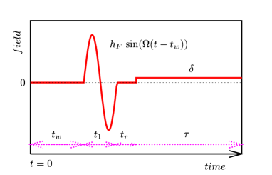
FIG. 1.: Wait, pump, recovery and probe scheme.

The NSHB technique has been first applied to the study of supercooled liquids. The polarization response of dielectric samples, glycerol and propylene carbonate, was measured after being modified by an ac electric field.[2] More recently, ion-conducting glasses like CKN [3], relaxor ferroelectrics (90PMN-10PT ceramics) [4] and spin-glasses (5% Au:Fe) [5] were studied with similar methods. The results have been interpreted as evidence for the existence of spatial heterogeneities. We show here that their main features can be reproduced by a system with no spatial structure. We use one model, out of a family, that captures many of the experimentally observed features of super-cooled liquids and glasses as, for instance, a two-step equilibrium relaxation close and above $T_{c}$ [6], aging effects below $T_{c}$ [7], etc. The model is the $p$ spherical spin-glass [8], that is intimately related to the $F_{p-1}$ mode-coupling model [9]. It can be interpreted as a system of $N$ fully-connected continuous spins or as a model of a particles in an infinite dimensional random environment. [10] In both cases, no reference to a geometry in real space nor any identification of spatially distinguishable regions can be made.

In the presence of a uniform field, the model is

$$H_{J}[{\bf s}]=\sum_{i_{1}\leq\dots\leq i_{p}}J_{i_{1}\dots i_{p}}\;s_{i_{1}}\dots s_{i_{p}}+h\;\sum_{i=1}^{N}s_{i}\;.$$ (1)

The interactions $J_{i_{1}\dots i_{p}}$ are quenched independent random variables taken from a Gaussian distribution with zero mean and variance $[J^{2}_{i_{1}\dots i_{p}}]_{J}={\tilde{J}}^{2}p!/(2N^{p-1})$. $p$ is a parameter and we take $p=3$. Hereafter $[\;\;]_{J}$ represents an average over $P[J]$ and $\tilde{J}=1$. The continuous variables $s_{i}$ are constrained spherically $\sum_{i=1}^{N}s_{i}^{2}=N$. A stochastic evolution is given to $\textstyle s$, $\dot{s}_{i}(t)=-\delta_{s_{i}(t)}H_{J}[{\mathchoice{{\hbox{\boldmath$\displaystyle s$}}}{{\hbox{\boldmath$\textstyle s$}}}{{\hbox{\boldmath$\scriptstyle s$}}}{{\hbox{\boldmath$\scriptscriptstyle s$}}}}]+\xi_{i}(t)$ with $\xi_{i}$ a white noise with $\langle\xi_{i}\rangle=0$ and $\langle\xi_{i}(t)\xi_{i}(t^{\prime})\rangle=2T\delta(t-t^{\prime})$. When $N\to\infty$, standard techniques lead to a set of coupled integro-differential equations for the autocorrelation $NC(t,t^{\prime})\equiv\sum_{i=1}^{N}[\langle s_{i}(t)s_{j}(t^{\prime})\rangle]_{J}$ and the linear response $R(t,t^{\prime})\equiv\left.\sum_{i=1}^{N}\delta[\langle s_{i}(t)\rangle]_{J}/\delta\delta_{i}(t^{\prime})\right|_{\delta=0}$, with $\delta_{i}(t^{\prime})$ an infinitesimal perturbation modifying the energy at time $t^{\prime}$ according to $H\to H-\sum_{i}\delta_{i}s_{i}$. The dynamic equations read [11]

$$\partial_{t}C(t,t^{\prime})=-z(t)\,C(t,t^{\prime})+\frac{p}{2}\int_{0}^{t^{\prime}}dt^{\prime\prime}C^{p-1}(t,t^{\prime\prime})R(t^{\prime},t^{\prime\prime})$$ (2)

$$\;\;\;\;\;\;\;+\frac{p(p-1)}{2}\int_{0}^{t}dt^{\prime\prime}C^{p-2}(t,t^{\prime\prime})R(t,t^{\prime\prime})C(t^{\prime\prime},t^{\prime})$$ (3)

$$\;\;\;\;\;\;\;+2TR(t^{\prime},t)+h(t)\int_{0}^{t^{\prime}}dt^{\prime\prime}h(t^{\prime\prime})R(t^{\prime},t^{\prime\prime})\;,$$ (4)

$$\partial_{t}R(t,t^{\prime})=-z(t)\,R(t,t^{\prime})$$ (5)

$$\;\;\;\;\;\;\;+\frac{p(p-1)}{2}\int_{t^{\prime}}^{t}dt^{\prime\prime}C^{p-2}(t,t^{\prime\prime})R(t,t^{\prime\prime})R(t^{\prime\prime},t^{\prime})\;,$$ (6)

The Lagrange multiplier $z(t)$ enforces the spherical constraint and an integral equation for it follows from Eq. (4) and the condition $C(t,t)=1$. In deriving these equations, a random initial condition at $t_{0}=0$ has been used. It corresponds to an infinitely fast quench from equilibrium at $T=\infty$ to the working temperature $T$. The evolution continues in isothermal conditions.

In the absence of energy pumping, these models have a dynamic phase transition at a ($p$-dependent) critical temperature $T_{c}$, $T_{c}\sim 0.61$ for $p=3$. When an external ac-field is applied, it drives the system out-of-equilibrium and stationarity and FDT do not necessarily hold at any temperature. The question as to whether the clearcut dynamic transition survives under an oscillatory field is open and we do not address it here. We simply study the dynamics close to the critical temperature in the absence of the field by constructing a numerical solution to Eqs. (4) and (6) with a constant grid algorithm of spacing $\epsilon$. We present data for small spacings, typically $\epsilon=0.02$, to minimize the numerical errors. Due to the fact that Eqs. (4) and (6) include integrals ranging from $t_{0}=0$ to present time $t$, the algorithm is limited to a maximum number of iterations of the order of $8000$ that imposes a lower limit $\Omega\sim 2\pi/(8000\epsilon)\sim 0.1$ to the frequencies we use.

A word of caution concerning the scheme in Fig. 1 and the times involved is in order. For the purpose of collecting the data for each reference unmodified integrated response, the sample is prepared at the working temperature $T$ at $t_{0}=0$ and let freely evolve during a total waiting time $t_{w}+t_{1}+t_{r}$. Depending on $T$, this interval may or may not be enough to equilibrate the sample. ($t_{1}$ is chosen as $t_{1}=2\pi n_{c}/\Omega$ with $\Omega$ the angular velocity of the field that will be used to record the modified curve.) A constant infinitesimal probe $\delta$ is applied after $t_{w}+t_{1}+t_{r}$ to measure

$$\Phi(\tau)\equiv\int_{0}^{\tau}d\tau^{\prime}\,R(t_{w}+t_{1}+t_{r}+\tau,t_{w}+t_{1}+t_{r}+\tau^{\prime})\;.$$

As an abuse of notation we explicitate only the $\tau$ dependence and eliminate the possible $t_{w}+t_{1}+t_{r}$ dependence. The modified integrated response $\Phi^{*}$ is measured after waiting $t_{w}$, applying $n_{c}$ oscillations of duration $t_{1}=2\pi n_{c}/\Omega$, further waiting $t_{r}$, and only then applying the probe $\delta$. The effect of the ac perturbation is then quantified by studying the difference:

$$\Delta\Phi\equiv\Phi^{*}-\Phi\;.$$ (7)

We have examined $\Delta\Phi$ at $T=0.8>T_{c}$ and $T=0.59<T_{c}$. We pump one oscillation with $h_{F}=0.1$ and later check that this field is small enough to provoke a spectral modification that is linear in the absorbed energy (see Fig. 5 below). For simplicity, we start by choosing $t_{w}=t_{r}=0$. In Fig. 3 we show $\Delta\Phi$ against $\log\tau$ for different $\Omega$ at $T=0.8$. All the curves are bell-shaped and vanish both at short and long times. In panel a, the $\Omega$s are larger than a threshold value $\Omega_{c}\sim 1$. The height of the peak $\Delta\Phi_{m}\equiv\max(\Delta\Phi)$ decreases with increasing frequency reaching the limit $\Delta\Phi_{m}=0$ for $\Omega\to\infty$. In addition, the location of the peak $t_{m}$ moves towards longer times when $\Omega$ decreases. In panel b, $\Omega<\Omega_{c}$ and the behaviour of the height of the peak is the opposite, it decreases when $\Omega$ decreases and, within numerically errors, its position is either independent of $\Omega$ or it very smoothly moves towards shorter times for increasing $\Omega$. The nonmonotonic behaviour of $\Phi_{m}$ with $\Omega$ is a consequence of the interplay between $t_{\alpha}$, the $\alpha$ relaxation time, and $2\pi/\Omega$ the period of the oscillation. The term $\int_{0}^{\min(t^{\prime},t_{1})}dt^{\prime\prime}h(t^{\prime\prime})R(t^{\prime},t^{\prime\prime})$ in Eq. (4) controls the effect of the field and, clearly, vanishes in the limits $\Omega\to\infty$ and $\Omega\to 0$. The inversion then occurs at a frequency $\Omega_{c}$ that is of the order of $2\pi/t_{\alpha}$. These results qualitatively coincide with the measurements of the electric relaxation in CKN at $T<T_{g}$ in Fig 1 a and b of Ref. [3]. In Fig. 3 we show $\Delta\Phi$ against $\log\tau$ for different $\Omega$ at $T=0.59$. For all $\Omega$ we reproduced the situation of panel a in Fig. 3, as if $\Omega>\Omega_{c}$. We have not found a threshold $\Omega_{c}$, that has gone below the minimum $\Omega$ reachable with the algorithm.

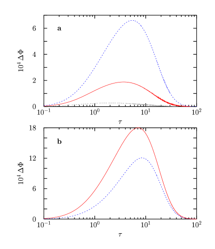
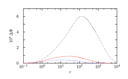
FIG. 2.: Time-difference dependence of the distortion $\Delta\Phi$ due to a single oscillation in a log-linear scale. $T=0.8>T_{c}$, $h_{F}=0.1$, $t_{w}=t_{r}=0$. At high pumping frequencies $\Omega>\Omega_{c}\sim 1$, shown in panel a, both the height of the peak $\Delta\Phi_{m}$ and its position $t_{m}$ decrease with increasing frequency. The dotted (blue), solid (red) and dashed (black) curves correspond to $\Omega=1,2,5$ respectively. In panel b, $\Omega<\Omega_{c}\sim 1$ and $\Delta\Phi_{m}$ increases with increasing $\Omega$ while $t_{m}$ is almost unchanged. The dotted (blue) and solid (red) curves correspond to $\Omega=0.1$ and $0.2$, respectively.

FIG. 3.: The same plot as in Fig. 3 for $T=0.59<T_{c}$. For all pumping frequencies explored, the peak moves towars shorter times and its height decreases for increasing frequencies. The dashed (black), solid (red) and dotted (blue) curves correspond to $\Omega=0.1,0.5$ and $1$, respectively.

The maximum modification of the relaxation $\Delta\Phi_{m}$ increases quadratically with the square of the amplitude of the pumping field $h_{F}$, and hence linearly in the absorbed energy, as long as $h_{F}\leq 1$. In Fig. 5 we display the relation $\Delta\Phi_{m}\propto h_{F}^{2}$ in a log-log scale for the two temperatures explored. The amplitude $h_{F}=0.1$ used in Figs. 3 and 3 is in the linear regime.

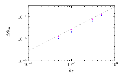
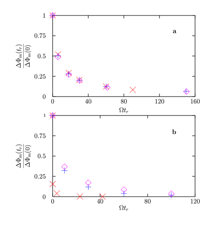
FIG. 4.: Check of $\Delta\Phi_{m}\propto h_{F}^{2}$ in a log-log scale. Squares (pink) correspond to $T=0.8$ and circles (blue) to $T=0.59$. In both cases one cycle of an ac-field with $\Omega=1$ was applied. The line has a slope equal to $2$ and is a guide-to-the-eye. The linear relation breaks down beyond $h_{F}\sim 1$.

FIG. 5.: The normalized maximum distortion for several recovery times $t_{r}$. In panel a $T=0.59$ and crosses, diamonds and pluses correspond to $\Omega=1,2$ and $3$, respectively. In panel b $T=0.8$ and crosses, pluses and diamonds correspond to $\Omega=1,5,10$, respectively.

The effect of the pump diminishes with increasing recovery time $t_{r}$. A convenient way of displaying this result is to plot the normalized maximum deviation $\Delta\Phi_{m}(t_{r})/\Delta\Phi_{m}(0)$ vs $\Omega t_{r}$. Using several frequencies and recovery times, we verified that this scaling holds for $T=0.59$ but does not hold for $T=0.8$, as shown in Fig. 5. This simple saling holds very nicely in the relaxor ferroelectric [4] and in the spin-glass [5] but it is very different from the $\Omega$-independence of the propylene carbonate [2].

Up to now, the effect of a single cycle of different frequencies has been studied. Another procedure can be envisaged. Since $t_{1}=2\pi n_{c}/\Omega$, we can change $t_{1}$ by applying different numbers of cycles $n_{c}$ while keeping $\Omega$ fixed. In Fig. 7 we show the distortion due to $n_{c}=10,2,1$ cycles with $\Omega=10$ at $T=0.8$. The qualitative dependence on $n_{c}$ is indeed the same as the dependence on $1/\Omega$: the peaks are displaced towards longer times with increasing $n_{c}$ (longer $t_{1}$). This behaviour is similar to the results obtained for propylene carbonate in Fig. 11 of Ref. [2]b. though we do not reach the expected saturation within our accessible time window.

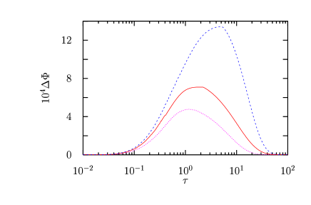
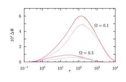
FIG. 6.: Effect of several cycles at $T=0.8$ for $\Omega=10$. The dashed (blue), solid (red) and dotted (pink) curves correspond to $n_{c}=10,2,1$ respectively.

FIG. 7.: Distortion for $t_{w}=8$ with dots (pink) compared with the one for $t_{w}=0$ with full line (red) at $T=0.59$.

Below $T_{c}$ the nonperturbed model never equilibrates and the relaxation depends on $t_{w}$. Indeed, $t_{\alpha}$ is an approximately linear function of $t_{w}$[7, 10] and the distortion might depend on $t_{w}$. We compare $\Delta\Phi$ vs $\log\tau$ for two $t_{w}$’s in Fig. 7.

Finally, we checked that the effect of one or many pump oscillations on the difference $\Delta C\equiv C^{*}(t_{w}+t_{1}+t_{r}+\tau,t_{w}+t_{1}+t_{r})-C(t_{w}+t_{1}+t_{r}+\tau,t_{w}+t_{1}+t_{r})$ is very similar to the one observed in $\Delta\Phi$. This observation is interesting since it is easier to compute numerically correlations than responses. Figure 8 shows the modification observed at $T=0.8$ and $\Omega>\Omega_{c}$ (to be compared to Fig. 3).

We conclude by stressing that we do not claim that spatial heterogeneities do not exist in real glassy systems. We just wish to stress that the ambiguities in the interpretation of experimental results have to be eliminated in order to have unequivocal evidence for them. The detailed comparison of the experimental measurements to the behaviour of glassy models with and without space will certainly help us refine the experimental techniques. Numerical simulations can play an important role in this respect.

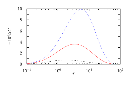
FIG. 8.: Change in the autocorrelation. $T=0.8$ and $\Omega=1$ (dashed blue), $\Omega=2$ (solid red) and $\Omega=5$ (dotted black).

LFC and JLI thank the Dept. of Phys. (UNMDP) and LPTHE (Jussieu) for hospitality, and ECOS-Sud, CONICET and UNMDP for financial support. We thank R. Böhmer, H. Cummins, G. Diezemann, M. Ediger, J. Kurchan and G. Mc Kenna for very useful discussions and T. Grigera, N. Israeloff and E. Vidal-Russel for introducing us to the hole-burning experiments.

REFERENCES

- [1] H. Sillescu, J. Non-Cryst. Solids, 243, 81 (1999). M. T. Cicerone and M. D. Ediger, J. Chem. Phys. 103, 5684 (1995). R. Böhmer et al, J. Non-Cryst. Solids 235-237 I-9 (1998).
- [2] a. B. Schiener et al Science 274, 752 (1996). b. B. Schieneret al J. Chem. Phys. 107, 7746 (1997).
- [3] R. Richert and R Böhmer, Phys. Rev. Lett. 83, 4337 (1999).
- [4] O. Kircher, B. Schiener and R. Böhmer, Phys. Rev. Lett. 20, 4520 (1998).
- [5] R. V. Chamberlin, Phys. Rev. Lett. 24, 5134 (1999).
- [6] W. Götze, J. Phys. C11, A1 (1999).
- [7] L. F. Cugliandolo and J. Kurchan, Phys. Rev. Lett. 71, 173 (1993).
- [8] A. Crisanti and H.-J. Sommers, Z. Phys. B87, 341 (1992).
- [9] T. R. Kirkpatrick and D. Thirumalai, Phys. Rev. B36, 5388 (1987).
- [10] For a review see J-P Bouchaud, L. F. Cugliandolo, J. Kurchan and M. Mézard, in Sping glasses and random fields, A. P. Young ed. (World Scientific, 1998).
- [11] L. F. Cugliandolo and J. Kurchan, Phys. Rev. B60, 922 (1999).