Multifractality of Entangled Random Walks and Nonuniform Hyperbolic Spaces

Abstract

Multifractal properties of the distribution of topological invariants for a model of trajectories randomly entangled with a nonsymmetric lattice of obstacles are investigated. Using the equivalence of the model to random walks on a locally nonsymmetric tree, statistical properties of topological invariants, such as drift and return probabilities, have been studied by means of a renormalization group (RG) technique. The comparison of the analytical RG–results with numerical simulations as well as with the rigorous results of P.Gerl and W.Woess [15] demonstrates clearly the validity of our approach. It is shown explicitly by direct counting for the discrete version of the model and by conformal methods for the continuous version that multifractality occurs when local uniformity of the phase space (which has an exponentially large number of states) has been broken.

I Introduction

The phenomenon of multifractality consists in a scale dependence of critical exponents. It has been widely discussed in the literature for a wide range of issues, such as statistics of strange sets [1], diffusion limited aggregation [2], wavelet transforms [3], conformal invariance [4] or statistical properties of critical wave functions of massless Dirac fermions in a random magnetic field [5, 6, 7].

The aim of our work is not only to describe a new model possessing multiscaling dependence, but also to show that the phenomenon of multifractality is related to local nonuniformity of the exponentially growing (”hyperbolic”) underlying ”target” phase space, through an example of entangled random walks distribution in homotopy classes. Indeed, to our knowledge, almost all examples of multifractal behavior for physical [5, 6, 7] or more abstract [1, 8] systems share one common feature—all target phase spaces have a noncommutative structure and are locally nonuniform.

We believe that multiscaling is a much more generic physical phenomenon compared with uniform scaling, appearing when the phase space of a system possesses a hyperbolic structure with local symmetry breaking. Such perturbation of local symmetry could be either regular or random—from our point of view the details of the origin of local nonuniformity play a less significant role.

We discuss below the basic features of multifractality in a locally nonuniform regular hyperbolic phase space. We show in particular that a multifractal behavior is encountered in statistical topology in the case of entangled (or knotted) random walks distribution in topological classes.

The paper is organized as follows. In Section II we consider a 2D $N$–step random walk in a nonsymmetric array of topological obstacles and investigate the multiscaling properties of the “target” phase space for a set of specific topological invariants—the “primitive paths”. The renormalization group computations of mean length of the primitive path, as well as return probabilities to the unentangled topological state are developed in Section III. Section IV is devoted to the application of conformal methods to a geometrical analysis of multifractality in locally nonuniform hyperbolic spaces.

II Multifractality of topological invariants for random entanglements in a lattice of obstacles

The concept of multifractality has been formulated and clearly explained in the paper [1]. We begin by recalling the basic definitions of Rényi spectrum, which will be used in the following.

Let $\nu(C_{i})$ be an abstract invariant distribution characterizing the probability of a dynamical system to stay in a basin of attraction of some stable configuration $C_{i}$ $(i=1,2,\ldots,{\cal N})$. Taking a uniform grid parameterized by ”balls” of size $l$, we define the family of fractal dimensions $D_{q}$:

$$D_{q}=\frac{1}{q-1}\lim_{l\to 0}\frac{\displaystyle\ln\sum_{i=1}^{\cal N}\nu^{q}(C_{i})}{\ln l}$$ (1)

As $q$ is varied, different subsets of $\nu^{q}$ associated with different values of $q$ become dominant.

Let us define the scaling exponent $\alpha$ as follows

$$\nu^{q}(C_{i})\sim l^{\alpha\,q}$$

where $\alpha$ can take different values corresponding to different regions of the measure which become dominant in Eq.(1). In particular, it is natural to suggest that $\sum_{i=1}^{\cal N}\nu^{q}(C_{i})$ can be rewritten as follows:

$$\sum_{i=1}^{\cal N}\nu^{q}(C_{i})=\left.\left[\int d\alpha^{\prime}\rho(\alpha^{\prime})l^{-f(\alpha^{\prime})}l^{\alpha^{\prime}\,q}\right]\right|_{l\to 0}$$

where $\rho(\alpha)$ is the probability to have the value $\alpha$ lying in a small ”window” $[\alpha^{\prime},\,\alpha^{\prime}+\Delta\alpha^{\prime}]$ and $f(\alpha)$ is a continuous function which has sense of fractal dimension of the subset characterized by the value $\alpha$.

Supposing $\rho(\alpha)>0$ one can approximately evaluate the last expression via the saddle–point method. Thus, one gets (see, for example, [1]):

$$\begin{array}[]{l}\displaystyle\frac{d}{d\alpha}f(\alpha)=q\vskip 6.0pt plus 2.0pt minus 2.0pt\\ \displaystyle\frac{d^{2}}{d\alpha^{2}}f(\alpha)<0\end{array}$$

what together with (1) leads to the following equations

$$\begin{array}[]{l}\displaystyle\tau(q)=q\alpha(q)-f[\alpha(q)]\vskip 6.0pt plus 2.0pt minus 2.0pt\\ \displaystyle\alpha(q)=\frac{d}{\displaystyle dq}\tau(q)\end{array}$$ (2)

where $\tau(q)=(q-1)D_{q}$. Hence, the exponents $\tau(q)$ and $f[\alpha(q)]$ are related via Legendre transform. For further details and more advanced mathematical analysis, the reader is refered to [9].

A 2D topological systems and their relation to hyperbolic geometry

Topological constraints essentially modify physical properties of the broad class of statistical systems composed of chain–like objects. It should be stressed that topological problems are widely investigated in connection with quantum field and string theories, 2D gravitation, statistics of vortices in superconductors, quantum Hall effect, thermodynamic properties of entangled polymers etc. Modern methods of theoretical physics allow us to describe rather comprehensively the effects of nonabelian statistics on the physical behavior of some systems. However the following question remains still obscure: what are the fractal (and as it is shown below, multifractal) properties of the distribution function of topological invariants, characterizing the homotopy states of a statistical system with topological constraints? We investigate this problem in the framework of the model ”Random Walk in an Array of Obstacles” (RWAO).

The RWAO–model can be regarded as physically clear and as a very representative image for systems of fluctuating chain–like objects with a full range of nonabelian topological properties. This model is formulated as follows: suppose that a random walk of $N$ steps of length $a$ takes place on a plane between obstacles which form a simple 2D rectangular lattice with unit cell of size $c_{x}\times c_{y}$. We assume that the random walk cannot cross (”pass through”) any obstacles.

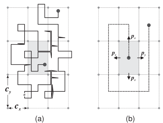
FIG. 1.: Random walk in the two-dimensional rectangular lattice of obstacles.

It is convenient to begin with the lattice realization of the RWAO–model. In this case the random path can be represented as a $N$–step random walk in a square lattice of size $a\times a$ ($a\leq c_{y}\leq c_{x}$)—see fig.1.

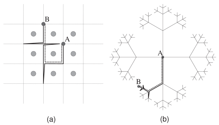
FIG. 2.: Random path for $a=c_{x}=c_{y}$: (a) in the 2D lattice of obstacles; (b) in the covering space (on the Cayley tree).

It had been shown previously (see, for example [10, 11]) that for $a=c_{x}=c_{y}$ a lattice random walk in the presence of a regular array of obstacles (punctures) on the dual lattice ${{\sf Z\kern-4.49997ptZ}}^{2}$ is topologicaly equivalent to a free random walk on a graph—a Cayley tree with branching number $z=4$ (see Fig.2). An outline of the derivation of this result is as follows. The different topological states of our problem coincide with the elements of the homotopy group of the multi-punctured plane, which is the free group $\Gamma_{\infty}$ generated by a countable set of elements. The translational invariance allows to consider a local basis and therefore to study the factored group $\Gamma_{\infty}/{{\sf Z\kern-4.49997ptZ}}^{2}=\Gamma_{z/2}$, where $\Gamma_{z/2}$ is a free group with $z/2$ generators whose Cayley graph is precisely a $z$–branching tree.

The relation between Cayley trees and hyperbolic geometry is discussed in details in Section III. Intuitively such a relation could be understood as follows. The Cayley tree can be isometrically embedded in the hyperbolic plane ${\cal H}$ (surface of constant negative curvature). The group $\Gamma_{z/2}$ is one of the discrete subgroups of the group of motion of the hyperbolic plane ${\cal H}=SL(2,{{\sf I\kern-1.49994ptR}})/SO(2)$, therefore the Cayley tree can be considered as a particular discrete realization of the hyperbolic plane.

Returning to the RWAO–model, we conclude that each trajectory in the lattice of obstacles can be lifted to a path in the “universal covering space” i.e to a path on the $z$–branching Cayley tree. The geodesic on the Cayley graph, i.e the shortest trajectory along the graph which connects ends of the path, plays the role of a complete topological invariant for the original trajectory in the lattice of obstacles. For example, the random walk in the lattice of obstacles is closed and contractible to a point (i.e. is not entangled with the array of obstacles) if and only if the geodesic length between the ends of the trajectory on the Cayley graph is zero. Hence, this geodesic length can be regarded as a topological invariant, which preserves the main nonabelian features of the considered problem.

We would like to stress two facts concerning our model: (i) The exact configuration of a geodesic is a complete topological invariant, while its length $k$ is only a partial topological invariant (except the case $k=0$); (ii) Geodesics have a clear geometrical interpretation, having sense of a bar (or ”primitive”) path which remains after deleting all even times folded parts of a random trajectory in the lattice of obstacles. The concept of ”primitive path” has been repeatedly used in statistical physics of polymers, leading to a successful classification of the topological states of chain–like molecules in various topological problems [10, 11, 12].

Even if many aspects of statistics of random walks in fixed lattices of obstacles have been well understood (see, for example [13] and references therein), the set of problems dealing with the investigation of fractal properties of the distribution of topological invariants in the RWAO–model are practically out of discussion. Thus we devote the next Section to the study of fractal and multifractal structures of the measure on the set of primitive paths in the RWAO–model for $a\ll c_{y}<c_{x}$.

B Multifractality of the measure on the set of primitive paths on a nonsymmetric Cayley tree

The classification of different topological states of a $N$–step random walk in a rectangular lattice of obstacles in the case $a\ll c_{y}<c_{x}$ turns out to be a more difficult and more rich problem than in the case $a=c_{y}=c_{x}$ discussed above. However, after a proper rescaling, the mapping of a random walk in the rectangular array of obstacles to a random walk on a Cayley tree can be explored again. To proceed we should solve two auxiliary problems. First of all we consider a random walk inside the elementary rectangular cell of the lattice of obstacles. Let us compute:

(i) The ”waiting time”, i.e the average number of steps $\left<t\right>$ which a $t$–step random walk spends within the rectangle of size $c_{x}\times c_{y}$;

(ii) The ratio of the ”escape probabilities” $p_{x}$ and $p_{y}$ through the corresponding sides $c_{x}$ and $c_{y}$ for a random walk staying till time $t$ within the elementary cell.

The desired quantities can be easily computed from the distribution function $P(x_{0},y_{0},x,y,t)$ which gives the probability to find the $t$–step random walk with initial $(x_{0},y_{0})$ and final $(x,y)$ points within the rectangle of size $c_{x}\times c_{y}$. The function $P(x,y,t)$ in the continuous approximation ($a\to 0;\,t\to\infty;\,at={\rm const}$) is the solution of the following boundary problem

$$\left\{\begin{array}[]{l}\displaystyle\frac{\partial}{\partial t}P(x,y,t)=\frac{a^{2}}{4}\left(\frac{\partial^{2}}{\partial x^{2}}+\frac{\partial^{2}}{\partial y^{2}}\right)P(x,y,t)\vskip 6.0pt plus 2.0pt minus 2.0pt\\ P(0,y,t)=P(c_{x},y,t)=P(x,0,t)=P(x,c_{y},t)=0\vskip 6.0pt plus 2.0pt minus 2.0pt\\ P(x,y,0)=\delta(x_{0},y_{0})\end{array}\right.$$ (3)

where $a$ is the length of the effective step of the random walk and the value $\frac{a^{2}}{4}$ has sense of a diffusion constant.

The solution of Eqs.(3) reads

$$P(x_{0},y_{0},x,y,t)=\frac{4}{c_{x}\;c_{y}}\sum_{m_{x}=1}^{\infty}\sum_{m_{y}=1}^{\infty}e^{-\frac{\pi^{2}a^{2}}{4}\left(\frac{m_{x}^{2}}{c_{x}^{2}}+\frac{m_{y}^{2}}{c_{y}^{2}}\right)t}\;\sin\frac{\pi m_{x}x_{0}}{c_{x}}\;\sin\frac{\pi m_{y}y_{0}}{c_{y}}\;\sin\frac{\pi m_{x}x}{c_{x}}\;\sin\frac{\pi m_{y}y}{c_{y}}$$ (4)

The ”waiting time” $\left<t\right>$ can be written now as follows

$$\left<t\right>=\frac{1}{c_{x}\;c_{y}}\int_{0}^{c_{x}}dx_{0}\int_{0}^{c_{y}}dy_{0}\int_{0}^{c_{x}}dx\int_{0}^{c_{y}}dy\int_{0}^{\infty}dt\;P(x_{0},y_{0},x,y,t)$$ (5)

while the ratio $p_{x}/p_{y}$ can be computed straightforwardly via the relation:

$$\frac{p_{x}}{p_{y}}=\frac{\displaystyle\left.\int_{0}^{c_{x}}dx_{0}\int_{0}^{c_{y}}dy_{0}\int_{0}^{c_{x}}dx\;P(x_{0},y_{0},x,y,t)\,\right|_{y=\{a,c_{y}-a\}}}{\displaystyle\left.\int_{0}^{c_{x}}dx_{0}\int_{0}^{c_{y}}dy_{0}\int_{0}^{c_{y}}dy\;P(x_{0},y_{0},x,y,t)\,\right|_{x=\{a,c_{x}-a\}}}$$ (6)

In the ”ground state dominance” approximation we truncate the sum (4) at $m_{x}=m_{y}=1$ and get the following approximate expressions:

$$\left<t\right>=\frac{4^{4}\,c_{x}^{2}\,c_{y}^{2}}{\pi^{6}\,a^{2}\,(c_{x}^{2}+c_{y}^{2})};\qquad\frac{p_{x}}{p_{y}}=\frac{c_{x}^{2}}{c_{y}^{2}}$$ (7)

In the symmetric case ($c_{x}=c_{y}\equiv c$) Eq.(7) gives $\left<t\right>=\frac{2^{7}\,c^{2}}{\pi^{6}\,a^{2}}$ and $p_{x}/p_{y}=1$, as it should be for the square lattice of obstacles.

Now the distribution function of the primitive paths for the RWAO model can be obtained via lifting this topological problem to the problem of directed random walks on the 4–branching Cayley tree, where the random walk on the Cayley tree is defined as follows:

(a) The total number of steps $\tilde{N}$ on the Cayley tree is

$$\tilde{N}=\frac{N}{\left<t\right>}=\frac{\pi^{6}}{4^{4}}\,\frac{Na^{2}(c_{x}^{2}+c_{y}^{2})}{c_{x}^{2}\,c_{y}^{2}}$$

(the value $\left<t\right>$ has been computed in (7)).

(b) The distance (or ”level” $k$) on the Cayley tree is defined as the number of steps of the shortest path between two points on the tree. Each vertex of the Cayley tree has 4 branches; the steps along two of them carry a Boltzmann weight $1$, while the steps along the two remaining ones carry a Boltzmann weight $\beta$ as it is shown in Fig.3. The value of $\beta$ is fixed by Eq.(7), which yields

$$\beta=\frac{p_{x}}{p_{y}}=\frac{c_{x}^{2}}{c_{y}^{2}}$$ (8)

The ultrametric structure of the topological phase space, i.e. of the Cayley tree $\gamma(\beta)$, allows us to use the results of paper [1] for investigating multicritical properties of the measure of all primitive (directed) paths of $k$ steps along the graph $\gamma(\beta)$ with nonsymmetric weights $1$ and $\beta$ (see Fig.3). A rigorous mathematical description of such weighted paths on trees (called cascades) can be found in [25], where the authors derive multifractal spectra, but for different distributions of weights.

FIG. 3.: 4–branching Cayley tree with different transition probabilities along branches.

We construct the partition function $\Omega(\beta,k)$ which counts properly the weighted number of all $4\times 3^{k-1}$ different $k$–step primitive paths on the graph $\gamma(\beta)$.

Define two partition functions $a_{k}$ and $b_{k}$ of $k$–step paths, whose last steps carry the weights $1$ and $\beta$ correspondingly. These functions satisfy the recursion relations for $k\geq 1$:

$$\left\{\begin{array}[]{l}a_{k+1}=a_{k}+2\,b_{k}\\ b_{k+1}=2\beta\,a_{k}+\beta\,b_{k}\end{array}\right.\qquad(k\geq 1)$$ (9)

with the following initial conditions at $k=1$:

$$\left\{\begin{array}[]{l}a_{1}=2\\ b_{1}=2\beta\end{array}\right.$$ (10)

Combining (9) and (10) we arrive at the following 2–step recursion relation for the function $a_{k}$:

$$\left\{\begin{array}[]{ll}a_{k+2}=(1+\beta)\,a_{k+1}+3\beta\,a_{k}&\qquad(k\geq 1)\\ a_{1}=2&\qquad(k=1)\\ a_{2}=2+4\beta&\qquad(k=2)\end{array}\right.$$ (11)

whose solution is

$$a_{k}=\frac{a_{2}-a_{1}\lambda_{2}}{\lambda_{1}-\lambda_{2}}\;\lambda_{1}^{k-1}+\frac{a_{1}\lambda_{1}-a_{2}}{\lambda_{1}-\lambda_{2}}\;\lambda_{2}^{k-1}$$ (12)

where

$$\lambda_{1,2}=\frac{1}{2}\left(1+\beta\pm\sqrt{(1+\beta)^{2}+12\beta}\right)$$ (13)

Taking into account that $b_{k}$ is given by the same recursion relation as $a_{k}$ but with the initial values $b_{1}=2\beta$ and $b_{2}=2\beta^{2}+4\beta$, we get the following expression for the partition function $\Omega(\beta,k)=a_{k}+b_{k}$:

$$\Omega(\beta,k)=\frac{2(1+4\beta+\beta^{2})-2(1+\beta)\lambda_{2}}{\lambda_{1}-\lambda_{2}}\;\lambda_{1}^{k-1}+\frac{2(1+\beta)\lambda_{1}-2(1+4\beta+\beta^{2})}{\lambda_{1}-\lambda_{2}}\;\lambda_{2}^{k-1}$$ (14)

The partition function $\Omega(\beta,k)$ contains all necessary information about the multifractal behavior. Following Eqs.(1)–(2), we associate the set of stable configurations $\{C_{i}\}$ with the set of ${\cal N}(k)=4\times 3^{k-1}$ vertices of level $k$. Hence, we define

$$\sum_{i=1}^{\cal N}\nu^{q}(C_{i})=\frac{\Omega(\beta^{q},k)}{\Omega^{q}(\beta,k)}$$ (15)

FIG. 4.: Dependence $D_{q}(q)$ for different values of Boltzmann weight $\beta$.

Taking into account that the uniform grid has resolution $l(k)=1/{\cal N}(k)$ for $k\geq 1$ and using Eq.(1), we obtain

$$\tau(q)=\lim_{k\to\infty}\frac{\ln\Omega(\beta^{q},k)-q\ln\Omega(\beta,k)}{\ln l(k)}$$ (16)

which allows to determine the generalized Hausdorff dimension $D_{q}$ via the relation

$$D_{q}=\tau(q)/(q-1)$$ (17)

The corresponding plots of the functions $D_{q}(q)$ for different values of $\beta=\{0.001;\,0.01;\,0.1;\,0.5\}$ are shown in Fig.4 (the numerical computations of Eqs.(16)–(17) are carried out for $k=100\,000$). The fact that $D_{q}(q)$ depends on $q$ clearly demonstrate the multifractal behavior.

III Random walk on a nonsymmetric Cayley tree

A Master equation

Consider a random walk on a 4-branching Cayley tree and investigate the distribution $P(k,\tilde{N})$ giving the probability for a $\tilde{N}$–step random walk starting at the origin of the tree to have a primitive (shortest) path between ends of length $k$. The random walk is defined as follows: at each vertex of the Cayley tree the probability of a step along two of the branches is $p_{x}$, and is $p_{y}$ along the two others; $p_{x}$ and $p_{y}$ satisfy the conservation condition $2p_{x}+2p_{y}=1$. Using Eq.(8), the following expressions hold:

$$\left\{\begin{array}[]{l}\displaystyle p_{x}=\frac{\beta}{2(1+\beta)}\vskip 6.0pt plus 2.0pt minus 2.0pt\\ \displaystyle p_{y}=\frac{1}{2(1+\beta)}\end{array}\right.$$ (18)

The symmetric case $\beta=1$ (which gives $p_{x}=p_{y}=1/4$) has already been studied and an exact expression for $P(k,\tilde{N})$ has been derived in [14]. The rigorous mathematical description of random walks on graphs can be found in [16]. Importance of spherical symmetry (i-e the fact that all vertices of a given level are strictly equivalent) is discussed in [23]. Another example of nonsymmetric model on a tree (case of randomly distributed transition probabilities, the so-called RWRE model) is described in [24]. To our knowledge, the solution for the nonsymmetric random walk which we defined above is known only for $k$ fixed and $\tilde{N}\gg 1$ [15]. Here we consider the case $k\gg 1,\;\tilde{N}\gg 1$, and in particular we study the distribution in the neighborhood of the maximum. Breaking the symmetry by taking $\beta\neq 1$ affects strongly the structure of the problem, since then the phase space becomes locally nonuniform: we have now vertices of two different kinds, $x$ and $y$, depending on whether the step toward the root of the Cayley tree occurs with probability $p_{x}$ or $p_{y}$. In order to obtain a master equation for $P(k,\tilde{N})$, we introduce the new variables $L_{x}(k,\tilde{N})$ and $L_{y}(k,\tilde{N})$, which define the probabilities to be at the level $k$ in a vertex $x$ or $y$ after $\tilde{N}$ steps. We recursively define the same way the probabilities $L_{a_{1}...a_{n}}(k,\tilde{N})$, ($a_{i}=\{x,y\}$) to be at level $k$ in a vertex such that the sequence of vertices toward the root of the tree is $a_{1}...a_{n}$. One can see that the recursion depends on the total ”history” till the root point, what makes the problem nonlocal. The master equation for the distribution function $P(k,\tilde{N})$

$$\begin{array}[]{lll}P(k,\tilde{N}+1)&=&(2p_{x}+p_{y})L_{y}(k-1,\tilde{N})+(2p_{y}+p_{x})L_{x}(k-1,\tilde{N})+\\ &&p_{y}L_{y}(k+1,\tilde{N})+p_{x}L_{x}(k+1,\tilde{N})\end{array}$$ (19)

is coupled to the hierarchical set of functions $\{L_{x},L_{y};L_{xx},L_{xy},L_{yx},L_{yy};...;L_{a_{1}...a_{n}}\}$ which satisfy the following recursion relation

$$\begin{array}[]{lll}L_{a_{1}...a_{n}}(k,\tilde{N}+1)&=&(2-\delta_{a_{1},a_{2}})p_{a_{1}}L_{a_{2}...a_{n}}(k-1,\tilde{N})+\\ &&p_{x}L_{xa_{1}...a_{n}}(k+1,\tilde{N})+p_{y}L_{ya_{1}...a_{n}}(k+1,\tilde{N})\end{array}$$ (20)

where $a_{1}...a_{n}$ cover all sequences of any lengths ($\leq k$) in $x$ and $y$. In order to close this infinite system at an arbitrary order $n_{0}$ we make the following assumption: for any $n\leq n_{0}$ we have

$$\left.\frac{L_{a_{1}...a_{n}}(k,\tilde{N})}{P(k,\tilde{N})}\right|_{k\gg n_{0}\atop\tilde{N}\gg n_{0}}\longrightarrow\alpha_{a_{1}...a_{n}}$$ (21)

with $\alpha_{a_{1}...a_{n}}$ constant.

Using the approximation (21) we rewrite (19)–(20) for large $k$ and $\tilde{N}$ in terms of the function $P(k,\tilde{N})$ and constants $\alpha_{a_{1}...a_{n}}$ ($0<n\leq n_{0}$). Taking into account that

$$L_{a_{1}...a_{n}x}+L_{a_{1}...a_{n}y}=L_{a_{1}...a_{n}}$$

we arrive at $2^{n_{0}-1}$ independent recursion relations for one and the same function $P(k,\tilde{N})$, with $2^{n_{0}}-1$ independent unknown constants $\alpha_{a_{1}...a_{n_{0}}}$. In order to make this system self–consistent, one has to identify coefficients entering in different equations, what yields $2^{n_{0}}-2$ compatibility relations for the constants $\alpha_{a_{1}...a_{n_{0}}}$, and the system is still open. This fact means that all scales are involved and the evolution of $L_{a_{1}...a_{n}}$ depends on $L_{a_{1}...a_{n+1}}$, the evolution of $L_{a_{1}...a_{n+1}}$ depends on $L_{a_{1}...a_{n+2}}$ and so on. At each scale we need informations about larger scales. This kind of scaling problem naturally suggests to use a renormalization group approach, which is developed in the next Section.

To begin with the renormalization procedure, we need to estimate the values of the constants $\alpha_{a_{1}...a_{n_{0}}}$ for the first (i.e. the smallest) scale. Let us denote

$$\left\{\begin{array}[]{l}\alpha_{x}=\alpha\\ \alpha_{y}=1-\alpha\end{array}\right.$$

and define $\alpha_{xx},\alpha_{xy},\alpha_{yy},\alpha_{yx}$ as follows:

$$\left\{\begin{array}[]{l}\alpha_{xx}=v_{x}\alpha\\ \alpha_{yy}=v_{y}(1-\alpha)\\ \alpha_{xy}=(1-v_{x})\alpha\\ \alpha_{yx}=(1-v_{y})(1-\alpha)\end{array}\right.$$

Now we set

$$p_{x}\alpha_{xa_{1}...a_{n}}+p_{y}\alpha_{ya_{1}...a_{n}}=\Big{(}p_{x}\alpha+p_{y}(1-\alpha)\Big{)}\alpha_{a_{1}...a_{n}}$$ (22)

what means that we neglect the correlations between the constants $\alpha_{a_{1}...a_{n}}$ and $\alpha_{a_{2}...a_{n}}$ at different scales. As it is shown in the next Section, the renormalization group approach allows us to get rid of the approximation (22).

With (22) one can obtain the following generic master equation

$$P(k,\tilde{N}+1)=\frac{p_{a_{1}}\alpha_{a_{2}...a_{n}}}{\alpha_{a_{1}...a_{n}}}\,(2-\delta_{a_{1},a_{2}})P(k-1,\tilde{N})+\Big{(}\alpha p_{x}+(1-\alpha)p_{y}\Big{)}P(k+1,\tilde{N})$$ (23)

where $a_{1}...a_{n}$ again cover all possible sequences in $x$ and $y$. We have now $2^{n_{0}}-1$ unknown quantities with $2^{n_{0}}-1$ compatibility relations (23), what makes the system (23) closed.

For illustration, we derive the solution for $n_{0}=2$:

$$\left\{\begin{array}[]{l}\displaystyle P(k,\tilde{N}+1)=\frac{p_{x}}{v_{x}}P(k-1,\tilde{N})+\Big{(}\alpha p_{x}+(1-\alpha)p_{y}\Big{)}P(k+1,\tilde{N})\vskip 6.0pt plus 2.0pt minus 2.0pt\\ \displaystyle P(k,\tilde{N}+1)=\frac{2p_{x}(1-\alpha)}{\alpha(1-v_{x})}P(k-1,\tilde{N})+\Big{(}\alpha p_{x}+(1-\alpha)p_{y}\Big{)}P(k+1,\tilde{N})\vskip 6.0pt plus 2.0pt minus 2.0pt\\ \displaystyle P(k,\tilde{N}+1)=\frac{p_{y}}{v_{y}}P(k-1,\tilde{N})+\Big{(}\alpha p_{x}+(1-\alpha)p_{y}\Big{)}P(k+1,\tilde{N})\vskip 6.0pt plus 2.0pt minus 2.0pt\\ \displaystyle P(k,\tilde{N}+1)=\frac{2p_{y}\alpha}{(1-\alpha)(1-v_{y})}P(k-1,\tilde{N})+\Big{(}\alpha p_{x}+(1-\alpha)p_{y}\Big{)}P(k+1,\tilde{N})\end{array}\right.$$ (24)

Note that (24) displays clearly a ${{\sf Z\kern-4.49997ptZ}}_{2}$ symmetry: $p_{x}\to p_{y},\;\alpha\to-\alpha,\;v_{x}\to v_{y}$. Compatibility conditions for system (24) read:

$$\frac{p_{x}}{v_{x}}=\frac{p_{y}}{v_{y}}=\frac{2p_{x}(1-\alpha)}{\alpha(1-v_{x})}=\frac{2p_{y}\alpha}{(1-\alpha)(1-v_{y})}$$ (25)

which finally gives

$$\left\{\begin{array}[]{l}\displaystyle\alpha=\frac{-1-3\beta+\sqrt{1+14\beta+\beta^{2}}}{2(1-\beta)}\vskip 6.0pt plus 2.0pt minus 2.0pt\\ \displaystyle v_{x}=\frac{\alpha}{2-\alpha}\vskip 6.0pt plus 2.0pt minus 2.0pt\\ \displaystyle v_{y}=\frac{1-\alpha}{1+\alpha}\end{array}\right.$$ (26)

As it has been said above, without (22) the system (19)–(20) is open, giving a single equation for the unknown function $P(k,\tilde{N})$ depending on the unknown parameter $\alpha$:

$$\begin{array}[]{lll}P(k,\tilde{N}+1)&=&\Big{(}(2p_{x}+p_{y})(1-\alpha)+(2p_{y}+p_{x})\alpha\Big{)}P(k-1,\tilde{N})+\vskip 6.0pt plus 2.0pt minus 2.0pt\\ &&\Big{(}p_{y}(1-\alpha)+p_{x}\alpha\Big{)}P(k+1,\tilde{N})\end{array}$$ (27)

Eq.(27) describes a 1D diffusion process with a drift

$$\frac{\langle k\rangle}{\tilde{N}}\equiv\overline{k}=2\alpha p_{y}+2(1-\alpha)p_{x}$$ (28)

and a dispersion

$$\delta=\frac{\langle k-\langle k\rangle\rangle^{2}}{\tilde{N}}=1-4\Big{(}\alpha p_{y}+(1-\alpha)p_{x}\Big{)}^{2}$$ (29)

which provides for $k\gg 1$ and $\tilde{N}\gg 1$ the usual Gaussian distribution with nonzero mean (see [10]). The value of $\alpha$ obtained in (26) using the approximation (22) gives a fair estimate of the drift compared with the numerical simulations, as it is shown in Fig.5.

B Real space renormalization

In order to improve the results obtained above, we recover the information lost in the approximation (22) and take into account “interactions” between different scales. Namely, we follow the renormalization flow of the parameter $\alpha(l)$ at a scale $l$ supposing that a new effective step is a composition of $2^{l}$ initial lattice steps. Let us define:

• the probability $f_{a}(l)$ of going forth (with respect to the location of the root point of the Cayley tree) from a vertex of kind $a$;

• the probability $b_{a}(l)$ of going back (towards the root point of the Cayley tree) from a vertex of kind $a$;

• the probability $\alpha(l)$ of being at a vertex of kind $x$;

• the conditional probability $w_{a}(l)$ to reach a vertex of kind $a$ starting from a vertex of kind $a$ under the condition that the step is forth;

• the conditional probability $v_{a}(l)$ to reach a vertex of kind $a$ starting from a vertex of kind $a$ under the condition that the step is back;

• the effective length $d(l)$ of a composite step.

Then the drift $\overline{k}(l)$ at scale $l$ is given by (compare with 28):

$$\overline{k}(l)=d(l)\left[\alpha(l)\Big{(}f_{x}(l)-b_{x}(l)\Big{)}+\Big{(}1-\alpha(l)\Big{)}\Big{(}f_{y}(l)-b_{y}(l)\Big{)}\right]$$ (30)

We say that the problem is scale–independent if the flow $\overline{k}(l)$ is invariant under the decimation procedure, i.e. with respect to the renormalization group. We compute the flow counting the appropriate combinations of two steps, depending on the variable considered:

$$\begin{array}[]{lll}w_{a}(l+1)&=&\displaystyle\Big{(}1-w_{a}(l)\Big{)}\Big{(}1-w_{\bar{a}}(l)\Big{)}+w_{a}^{2}(l)\vskip 6.0pt plus 2.0pt minus 2.0pt\\ v_{a}(l+1)&=&\displaystyle\Big{(}1-v_{a}(l)\Big{)}\Big{(}1-v_{\bar{a}}(l)\Big{)}+v_{a}^{2}(l)\vskip 6.0pt plus 2.0pt minus 2.0pt\\ f_{a}(l+1)&=&\displaystyle\frac{f_{a}(l)\left[w_{a}(l)f_{a}(l)+\Big{(}1-w_{a}(l)\Big{)}f_{\bar{a}}(l)\right]}{c_{a}(l)}\vskip 6.0pt plus 2.0pt minus 2.0pt\\ b_{a}(l+1)&=&\displaystyle\frac{b_{a}(l)\left[v_{a}(l)b_{a}(l)+\Big{(}1-v_{a}(l)\Big{)}b_{\bar{a}}(l)\right]}{c_{a}(l)}\vskip 6.0pt plus 2.0pt minus 2.0pt\\ d(l+1)&=&\displaystyle d(l)\left[\alpha(l)c_{x}(l)+\Big{(}1-\alpha(l)\Big{)}c_{y}(l)\right]\vskip 6.0pt plus 2.0pt minus 2.0pt\\ \alpha(l+1)&=&\displaystyle\overline{k}(l)\left[\alpha(l)w_{x}(l)+\Big{(}1-\alpha(l)\Big{)}\Big{(}1-w_{y}(l)\Big{)}\right]+\vskip 6.0pt plus 2.0pt minus 2.0pt\\ &&\displaystyle\left(1-\overline{k}(l)\right)\left[\alpha(l)v_{x}(l)+\Big{(}1-\alpha(l)\Big{)}\Big{(}1-v_{y}(l)\Big{)}\right]\end{array}$$ (31)

where $\bar{a}=x$ when $a=y$ (and $\bar{a}=y$ when $a=x$) and the value $c_{a}(l)$ ensures the conservation condition $f_{a}(l+1)+b_{a}(l+1)=1$ because we do not consider the combinations of two successive steps in opposite directions.

The transformation of $\alpha$ in (31) needs some explanations. We consider the drift $\overline{k}(l)$ as a probability to make a (composite) step forward. The equation for $\alpha$ is given by counting the different ways of getting to a vertex of kind $x$. One can check that $\overline{k}(l)$ given by (30) remains invariant under such transformation, what is considered as a verification of the scale independence (i.e. of renormalizability).

Following the standard procedure, we find the fixed points for the flow of $\alpha(l)$. First of all we realize that the recursion equations for $w_{a}(l)$ and $v_{a}(l)$ can be solved independently, providing a continuous set of fixed points: $w_{x}^{0}=1-w_{y}^{0}$ and $v_{x}^{0}=1-v_{y}^{0}$. Using the initial conditions (26) for $v_{a}(l)$ and deriving straightforwardly the absent initial conditions for $w_{a}(l)$, we get

$$\left\{\begin{array}[]{l}v_{x}(1)=v_{x}\vskip 6.0pt plus 2.0pt minus 2.0pt\\ v_{y}(1)=v_{y}\vskip 6.0pt plus 2.0pt minus 2.0pt\\ \displaystyle w_{x}(1)=w_{x}=\frac{p_{x}}{p_{x}+2p_{y}}\vskip 6.0pt plus 2.0pt minus 2.0pt\\ \displaystyle w_{y}(1)=w_{y}=\frac{p_{y}}{p_{y}+2p_{x}}\end{array}\right.$$ (32)

(we recall that these values are obtained by taking into account the elementary correlations for two successive steps).

With the initial conditions (32) we find the following renormalized values $v^{0}$ and $w^{0}$ at the fixed point

$$\left\{\begin{array}[]{l}\displaystyle v^{0}=v^{0}(\beta)=\lim_{l\to\infty}v_{x}(l)=1-\lim_{l\to\infty}v_{y}(l)=\frac{1}{2}\left[(v_{x}-v_{y})\prod_{n=1}^{\infty}f^{(n)}(v_{x}+v_{y})+1\right]\vskip 6.0pt plus 2.0pt minus 2.0pt\\ \displaystyle w^{0}=w^{0}(\beta)=\lim_{l\to\infty}w_{x}(l)=1-\lim_{l\to\infty}w_{y}(l)=\frac{1}{2}\left[(w_{x}-w_{y})\prod_{n=1}^{\infty}f^{(n)}(w_{x}+w_{y})+1\right]\end{array}\right.$$ (33)

where $f^{(n)}(x)$ is the $n^{\rm th}$ iteration of the function

$$f(x)=x^{2}-2x+2$$

We then obtain successively all renormalized values at the fixed point

$$\left\{\begin{array}[]{l}f_{a}^{0}=1\vskip 6.0pt plus 2.0pt minus 2.0pt\\ b_{a}^{0}=0\vskip 6.0pt plus 2.0pt minus 2.0pt\\ \displaystyle d^{0}=\overline{k^{0}}=\frac{\alpha^{0}+\beta(1-\alpha^{0})}{1+\beta}\vskip 6.0pt plus 2.0pt minus 2.0pt\\ \displaystyle\alpha^{0}=\frac{v^{0}+\beta w^{0}}{1+\beta+(1-\beta)(v^{0}-w^{0})}\end{array}\right.$$ (34)

where the invariance of the drift $\overline{k}$ is taken into account:

$$\overline{k^{0}}=\overline{k}(1)=2p_{y}\alpha^{0}+2p_{x}(1-\alpha^{0})=\frac{\alpha^{0}+\beta(1-\alpha^{0})}{1+\beta}$$

FIG. 5.: The values of $\alpha$ and $\overline{k}$ compared to renormalized quantities and numerical simulations.

In figure 5 we compare the theoretical results with numerical simulations. It is worth mentioning the efficiency of the renormalization group method, which yields a solution in very good agreement with numerical simulations in a broad interval of values $\beta$.

In addition we compare our results with the exact expression obtained by P.Gerl and W.Woess in [15] for the probability $P(0,\tilde{N})$ to return to the origin after $\tilde{N}$ random steps on the nonsymmetric Cayley tree. This distribution function $P(0,\tilde{N})$ reads

$$P(0,\tilde{N})\propto\mu^{\tilde{N}}\,\tilde{N}^{-3/2}$$ (35)

with

$$\mu\equiv\mu(\beta)=\min\left\{-t+\sqrt{t^{2}+4p^{2}_{x}}+\sqrt{t^{2}+4p^{2}_{y}}\;\Big{|}t>0\right\}$$ (36)

Let us assert now without justification that Eq.(27) (which is actually written for $k\gg 1$ and $\tilde{N}\gg 1$) is valid for any values of $k$ and $\tilde{N}$. The initial conditions for the recursion relation (27) are as follows

$$\left\{\begin{array}[]{l}P(0,\tilde{N}+1)=\Big{(}2\alpha p_{x}+2(1-\alpha)p_{y}\Big{)}P(1,\tilde{N})\\ P(k,0)=\delta_{k,0}\end{array}\right.$$ (37)

One can notice that Eq.(27) completed with the conditions (37) can be viewed as a master equation for a symmetric random walk on a Cayley tree with effective branching $z$ continuously depending on $\beta$:

$$z(\beta)=\frac{2}{\alpha p_{x}+(1-\alpha)p_{y}}$$ (38)

Hence, we conclude that our problem becomes equivalent to a symmetric random walk on a $z(\beta)$-branching tree. For $k=0$ the solution, given in [10] is

$$P(0,\tilde{N})\propto\left[\frac{2\sqrt{z(\beta)-1}}{z(\beta)}\right]^{\tilde{N}}\,\tilde{N}^{-3/2}$$ (39)

This provides the same form as the exact solution (35). It has been checked numerically that for $\beta\in{\sf I\kern-1.49994ptR}^{+}$ the discrepancy between (35) and (39) is as follows

$$\frac{1}{\mu(\beta)}\left|\frac{2\sqrt{z(\beta)-1}}{z(\beta)}-\mu(\beta)\right|<0.02$$

Thus, we believe that our self–consistent RG–approach to statistics of random walks on nonsymmetric trees can be extended with sufficient accuracy to all values of $k$.

IV Multifractality and locally nonuniform curvature of Riemann surfaces

We have claimed in Sections I–II that local nonuniformity and the exponentially growing structure of the phase space of statistical systems generates a multiscaling behavior of the corresponding partition functions. The aim of the present Section is to bring geometric arguments to support our claim by introducing a different approach of the RWAO model. The differences between the approach considered in this Section and the one discussed in Section II are as follows:

• We consider a continuous model of random walk topologically entangled with either a symmetric or a nonsymmetric triangular lattice of obstacles on the plane.

• We pursue the goal to construct explicitly the metric structure of the topological phase space via conformal methods and to relate directly the nonuniform fractal relief of the topological phase space to the multifractal properties of the distribution function of topological invariants for the given model.

Consider a random walk in a regular array of topological obstacles on the plane. As in the discrete case we can split the distribution function of all $N$–step paths with fixed positions of end points into different topological (homotopy) classes. We characterize each topological class by a topological invariant similar to the ”primitive path” defined in Section II. Introducing complex coordinates $z=x+iy$ on the plane, we use conformal methods which provide an efficient tool for investigating multifractal properties of the distribution function of random trajectories in homotopy classes.

Let us stress that explicit expressions are constructed so far for triangular lattices of obstacles only. That is why we replace the investigation of the rectangular lattices discussed in Sections I–II by the consideration of the triangular ones. Moreover, for triangular lattices a continuous symmetry parameter (such as $\beta=c_{x}^{2}/c_{y}^{2}$ in case of rectangular lattices) does not exist and only the triangles with angles $(\pi/3,\pi/3,\pi/3)$, $(\pi/2,\pi/4,\pi/4)$, $(\pi/2,\pi/6,\pi/3)$ are available—only such triangles tessellate the whole plane $z$. In spite of the mentioned restrictions, the study of these cases enables us to figure out an origin of multifractality coming from the metric structure of the topological phase space.

Suppose that the topological obstacles form a periodic lattice in the $z$–plane. Let the fundamental domain of this lattice be the triangle $ABC$ with angles either $(\pi/3,\pi/3,\pi/3)$ (symmetric case) or $(\pi/2,\pi/6,\pi/3)$ (nonsymmetric case). The conformal mapping $z(\zeta)$ establishes a one-to-one correspondence between a given fundamental domain $ABC$ of the lattice of obstacles in the $z$–plane with a zero–angled triangle ${\cal ABC}$ lying in the upper half–plane $\eta>0$ of the plane $\zeta=\xi+i\eta$, and having corners on the real axis $\eta=0$. To avoid possible misunderstandings let us point out that such transform is conformal everywhere except at corner (branching) points—see, for example [17]. Consider now the tessellation of the $z$–plane by means of consecutive reflections of the domain $ABC$ with respect to its sides, and the corresponding reflections (inversions) of the domain ${\cal ABC}$ in the $\zeta$–plane. Few first generations are shown in Fig.6. The obtained upper half–plane ${\rm Im}\zeta>0$ has a ”lacunary” structure and represents the topological phase space of the trajectories entangled with the lattice of obstacles. The details of such a construction as well as a discussion of the topological features of the conformal mapping $z(\zeta)$ in the symmetric case can be found in [13]. We recall the basic properties of the transform $z(\zeta)$ related to our investigation of multifractality.

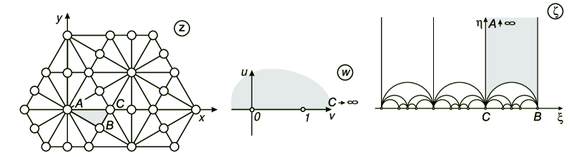
FIG. 6.: Conformal mapping of the complex plane $z$ to the ”lacunary” upper half–plane ${\rm Im}\zeta>0$ endowed with a Poincaré metric. The zero–angled triangle ${\cal ABC}$ on $\zeta$ corresponds to the triangle $ABC$ with the angles $(\pi/2,\pi/6,\pi/3)$ on $z$.

The topological state of a trajectory $C$ in the lattice of obstacles can be characterized as follows.

• Perform the conformal mappings $z_{\rm s}(\zeta)$ (or $z_{\rm ns}(\zeta)$) of the plane $z$ with symmetric (or nonsymmetric) triangular lattice of obstacles to the upper half-plane ${\rm Im}\zeta>0$, playing the role of the topological phase space of the given model.

• Connect by nodes the centers of neighboring curvilinear triangles in the upper half–plane ${\rm Im}\zeta>0$ and raise a graph $\gamma_{\rm s}$ (or $\gamma_{\rm ns}$) (which is, as shown below an isometric Cayley tree embedded in the Poincaré plane).

• Find the image of the path $C$ in the ”covering space” ${\rm Im}\zeta>0$ and define the shortest (primitive) path connecting the centers of the curvilinear triangles where the ends of the path $C$ are located. The configuration of this primitive path projected to the Cayley tree $\gamma_{\rm s}$ (or $\gamma_{\rm ns}$) plays the role of topological invariant for the model under consideration.

The Cayley trees $\gamma_{\rm s,ns}$ have the same topological content as the one described in the Section II, but here we determine the Boltzmann weights $\beta_{1},\beta_{2},\beta_{3}$ associated with passages between neighboring vertices (see Fig.7) directly from the metric properties of the topological phase space obtained via the conformal mappings $z_{\rm s,ns}(\zeta)$.

FIG. 7.: Nonsymmetric 3–branching Cayley tree.

It is well known that random walks are conformally invariant; in other words the diffusion equation on the plane $z$ preserves its structure under a conformal transform, but the diffusion coefficient can become space–dependent [18]. Namely, under the conformal transform $z(\zeta)$ the Laplace operator $\Delta_{z}=\frac{d^{2}}{dzd\overline{z}}$ is transformed in the following way

$$\frac{d^{2}}{dzd\overline{z}}=\frac{1}{|z^{\prime}(\zeta)|^{2}}\;\frac{d^{2}}{d\zeta d\overline{\zeta}}$$ (40)

Before discussing the properties of the Jacobians $|z^{\prime}(\zeta)|^{2}$ for the symmetric and nonsymmetric transforms, it is more convenient to set up the following geometrical context. The connection between Cayley trees and surfaces of constant negative curvature has already been pointed out [13], mostly through volume growth considerations. Therefore it becomes more natural to regard the upper half–plane ${\rm Im}\zeta>0$ as the standard realization of the hyperbolic 2–space (surface of constant negative curvature $R$, with here arbitrarily $R=-2$), that is to consider the following metric:

$$ds^{2}=\frac{-2}{R\eta^{2}}(d\xi^{2}+d\eta^{2})$$ (41)

Let us rewrite the Laplace operator (40) in the form

$$\frac{d^{2}}{dzd\overline{z}}=D(\xi,\eta)\;\eta^{2}\,\left(\frac{d^{2}}{d\xi^{2}}+\frac{d^{2}}{d\eta^{2}}\right)$$ (42)

where the value $D(\xi,\eta)\equiv D(\zeta)$ can be interpreted as the normalized space–dependent diffusion coefficient on the Poincaré upper half–plane:

$$D(\zeta)=\frac{1}{\eta^{2}\,|z^{\prime}(\zeta)|^{2}}$$ (43)

The methods providing the conformal transform $z_{\rm s}(\zeta)$ for the symmetric triangle with angles $(\pi/3,\pi/3,\pi/3)$ have been discussed in details in [17]. The generalization of these results to the conformal transform $z_{\rm ns}(\zeta)$ for the nonsymmetric triangle with angles $(\pi/2,\pi/6,\pi/3)$ is very straightforward. We here expose the Jacobians of those conformal mappings without derivation:

$$\begin{array}[]{l}\displaystyle\left|z_{\rm s}^{\prime}(\zeta)\right|^{2}=\frac{1}{\pi^{2/3}B^{2}\left(\frac{1}{3},\frac{1}{3}\right)}\;\left|\theta_{1}^{\prime}(0,e^{i\pi\zeta})\right|^{8/3}\vskip 6.0pt plus 2.0pt minus 2.0pt\\ \displaystyle\left|z_{\rm ns}^{\prime}(\zeta)\right|^{2}=\frac{\pi^{2}}{B^{2}\left(\frac{1}{2},\frac{1}{3}\right)}\left|\theta_{0}(0,e^{i\pi\zeta})\right|^{8/3}\;\left|\theta_{2}(0,e^{i\pi\zeta})\right|^{4}\;\left|\theta_{3}(0,e^{i\pi\zeta})\right|^{4/3}\end{array}$$ (44)

where $\theta_{1}^{\prime}(\chi|...)=\frac{d}{d\chi}\theta_{1}(\chi|...)$ and $\theta_{i}(0|...)$ $(i=0,...,3)$ are the standard definitions of Jacobi elliptic functions [19].

Combining (43) and (44) we define the effective inverse diffusion coefficients in symmetric ($D^{-1}_{\rm s}$) and in nonsymmetric ($D^{-1}_{\rm ns}$) cases:

$$\begin{array}[]{l}D^{-1}_{\rm s}(\zeta)=\eta^{2}\;\left|z^{\prime}_{\rm s}(\zeta)\right|^{2}\vskip 6.0pt plus 2.0pt minus 2.0pt\\ D^{-1}_{\rm ns}(\zeta)=\eta^{2}\;\left|z^{\prime}_{\rm ns}(\zeta)\right|^{2}\end{array}$$ (45)

The corresponding 3D plots of the reliefs $D^{-1}_{\rm s}(\xi,\eta)$ and $D^{-1}_{\rm s}(\xi,\eta)$ are shown in Fig.8.

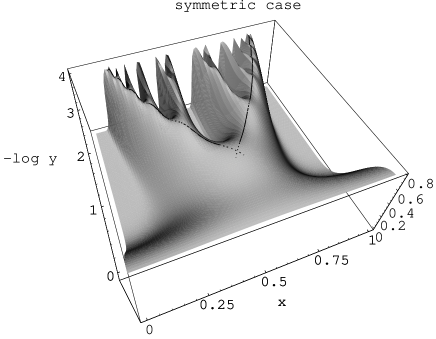
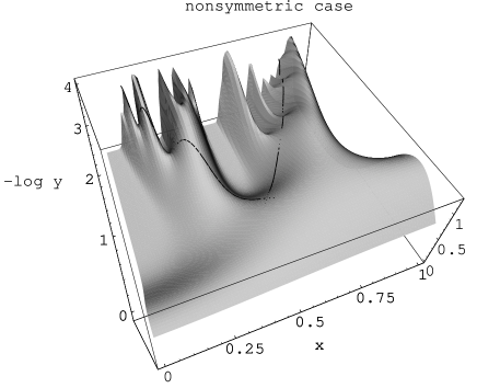
FIG. 8.: Profiles of the surfaces $D^{-1}_{\rm s}(\xi,\eta)$ and $D^{-1}_{\rm ns}(\xi,\eta)$ where $\xi\equiv x,\;\eta\equiv-\log y$. First generation of horocycles are shown by the lines.

The functions $D^{-1}_{\rm s}(\zeta)$ and $D^{-1}_{\rm ns}(\zeta)$ are considered as quantitative indicators of the topological structure of the phase spaces; in particular a Cayley tree can be isometrically embedded in the surface $D^{-1}_{\rm s}(\zeta)$. It can be shown that the images of the centers of the triangles of the symmetric lattice in the $z$–plane correspond to the local maxima of the surface $D^{-1}_{\rm s}(\zeta)$ in the $\zeta$–plane. We define the vertices of the embedded tree as those maxima. The links connecting neighboring vertices are defined in the next paragraph.

Let us define the horocycles which correspond to repeating sequences of weights in Fig.7 with minimal periods. There are only three such sequences: $\beta_{1}\beta_{2}\beta_{1}\beta_{2}...$,  $\beta_{1}\beta_{3}\beta_{1}\beta_{3}...$ and  $\beta_{2}\beta_{3}\beta_{2}\beta_{3}...$. The horocycles are images (analytically known) of certain circles of the $z$–plane. They proved to be a convenient tool for a constructive description of the trajectories in the $z$–plane starting from the trajectories in the covering space $\zeta$.

The first generation of horocycles (closest to the root point of the Cayley tree) is shown in Fig.8. Let us consider the symmetric case. Following a given horocycle we follow a ridge of the surface, and we pass through certain maxima of this surface (that is through certain vertices of the tree). We therefore define locally the links of the tree as the set of ridges connecting neighboring maxima of $D^{-1}_{\rm s}(\xi,\eta)$. We recall that the ridge of the surface can be defined as the set of points where the gradient of the function $D^{-1}_{\rm s}(\xi,\eta)$ is minimal along its isoline. Even if this gives a proper definition of the tree, extracting a direct parametrization is difficult, that is why henceforth we will approximate the tree by arcs of horocycles.

To give a quantitative formulation of the local definition of the embedded Cayley tree, we consider the path integral formulation of the problem on the $\zeta$–plane. Define the Lagrangian ${\cal L}\propto D^{-1}_{\rm s}(\zeta){\dot{\zeta}}^{2}$ of a free particle moving with the diffusion coefficient $D_{\rm s}(\zeta)$ in the space $\zeta$. Following the canonical procedure and minimizing the corresponding action [20], we get the equations of motion in the effective potential $U=\ln(\eta^{2}D_{\rm s})$:

$$\ddot{q}_{i}=({\dot{q}_{j}}\partial_{j}U){\dot{q}_{i}}-\frac{1}{2}{\dot{q}_{j}}{\dot{q}_{j}}\partial_{i}U$$ (46)

where $q_{1}=\xi$ and $q_{2}=\eta$. Even if Eq.(46) is nonlinear with a friction term, one can show that the trajectory of extremal action between the centers of two neighboring triangles follow the ridge of the surface $D_{\rm s}(\zeta)$.

It is noteworthy that obtaining an analytical support of Cayley graphs is of great importance, since those graphs clearly display ultrametric properties and have connections to $p$–adic surfaces [21]. The detailed study of metric properties of the functions $D^{-1}_{\rm s}(\zeta)$ and $D^{-1}_{\rm ns}(\zeta)$ is left for separate publication.

While the self–similar properties of the Jacobians of those conformal mappings appear clearly in Fig.8, one could wonder how the local symmetry breaking affects the continuous problem. We can see that if $D^{-1}_{\rm s}(\zeta)$ is univalued along the embedded tree, $D^{-1}_{\rm ns}(\zeta)$ does vary, what makes the tree locally nonuniform and leads to a multifractal behavior. In other words, different paths of same length along the tree have the same weights in the symmetric case, but have different ones in the nonsymmetric case. The probability of a random path $C$ of length $L$ can be written in terms of a path integral with a Wiener measure

$$p_{C}={\cal D}\{s\}\exp\left\{-\int_{0}^{L}\frac{1}{D[s(t)]}\left(\frac{ds}{dt}\right)^{2}dt\right\}$$ (47)

where $s(t)$ is a parametric representation of the path $C$.

The first horocycles in Fig.8 can be parameterized as follows

$$\left\{\begin{array}[]{l}\xi=\frac{1}{2}\pm(\frac{1}{2}-\frac{\sqrt{3}}{3}\sin\theta)\\ \eta=\frac{\sqrt{3}}{3}(1-\cos\theta)\end{array}\right.$$ (48)

with $\theta$ running in the interval $[0,\pi/2]$. The condition ensuring the constant velocity $\dot{s}\equiv\frac{ds}{dt}$ along the horocycles gives with (41)

$$\frac{1}{\eta}\;\frac{d\theta}{dt}={\rm const}$$

hence

$$\theta(t)=\arctan\left(\frac{1}{t}\right)$$ (49)

with proper choice of the time unit. This parameterization is used to check that the embedded tree is isometric. Indeed, the horocycles shown in Fig.8 correspond to a periodic sequence of steps like $\beta_{1}\beta_{2}\beta_{1}\beta_{2}...$, $\beta_{1}\beta_{3}\beta_{1}\beta_{3}...$ or $\beta_{2}\beta_{3}\beta_{2}\beta_{3}...$. It is natural to assert that a step carries a Boltzmann weight characterized by the corresponding local values of $D^{-1}_{\rm ns}$. Therefore the period of the plot shown in Fig.9 is directly linked to the spacing of the tree embedded in the profile $D^{-1}_{\rm ns}$.

FIG. 9.: $D^{-1}_{\rm ns}$ running along a horocycle at constant velocity. Periodicity shows that the tree is isometric.

Coming back to the probability of different paths covered at constant velocity, one can write

$$-\log p_{C}\propto\int_{t_{1}}^{t_{2}}\frac{dt}{D[s(t)]}$$ (50)

The figure 10 shows the value $-\log p_{C}$ in symmetric and nonsymmetric cases for different paths starting at $t_{1}=0^{+}$ and ending at $t$. In the symmetric case all plots are the same (solid line), whereas in the nonsymmetric case they are different: dashed and dot–dashed curves display the corresponding plots for the sequences $\beta_{2}\beta_{3}\beta_{2}\beta_{3}...$ and $\beta_{1}\beta_{3}\beta_{1}\beta_{3}...$.

Following the outline of construction of the fractal dimensions $D_{q}$ in Section II, we can describe multifractality in the continuous case by

$$D_{q}=-\frac{1}{q-1}\;\lim_{L\to\infty}\frac{1}{\ln{\cal N}(L)}\ln\frac{\displaystyle\int{\cal D}\{s\}\exp\left\{-q\int_{0}^{L}D^{-1}_{\rm ns}(s(t))dt\right\}}{\displaystyle\left[\int{\cal D}\{s\}\exp\left\{-\int_{0}^{L}D^{-1}_{\rm ns}(s(t))dt\right\}\right]^{q}}$$ (51)

where ${\cal N}(l)$ is the area of the surface covered by the trajectories of length $L$. This form is consistent with definitions 1 and 16. Indeed, if instead of the usual Wiener measure one chooses a discrete measure $d\chi_{T}$, which is nonzero only for trajectories along the Cayley tree, we recover the following description.

Define the distribution function $\Theta(\beta_{1},\beta_{2},\beta_{3},k)\equiv\Theta\left(\frac{\beta_{1}}{\beta_{3}},\frac{\beta_{2}}{\beta_{3}},k\right)$, which has sense of the weighted number of directed paths of $k$ steps on the nonsymmetric 3–branching Cayley tree shown in Fig.7. The values of the effective Boltzmann weights $\frac{\beta_{1}}{\beta_{3}}$ and $\frac{\beta_{2}}{\beta_{3}}$ are defined in terms of the local heights of the surface $D_{\rm ns}^{-1}$ along the corresponding branches of the embedded tree. We set

$$\begin{array}[]{l}\displaystyle\frac{\beta_{1}}{\beta_{3}}=\exp\left[\displaystyle\int_{t_{1}}^{t_{2}}\frac{dt}{D_{\rm ns}[s_{r}(t)]}-\int_{t_{2}}^{t_{3}}\frac{dt}{D_{\rm ns}[s_{r}(t)]}\right]\approx 1.07;\vskip 6.0pt plus 2.0pt minus 2.0pt\\ \displaystyle\frac{\beta_{2}}{\beta_{3}}=\exp\left[\displaystyle\int_{t_{1}}^{t_{2}}\frac{dt}{D_{\rm ns}[s_{l}(t)]}-\int_{t_{2}}^{t_{3}}\frac{dt}{D_{\rm ns}[s_{l}(t)]}\right]\approx 1.19\end{array}$$ (52)

where $t_{1},t_{2},t_{3}$ are adjusted so that $s_{r}(t)$ represents a step weighted with $\beta_{3}$ for $t_{1}<t<t_{2}$ and a step weighted with $\beta_{1}$ for $t_{2}<t<t_{3}$ for right–hand–side horocycles while $s_{l}(t)$ represents a step weighted with $\beta_{3}$ for $t_{1}<t<t_{2}$ and a step weighted with $\beta_{2}$ for $t_{2}<t<t_{3}$ for left–hand–side horocycles.

FIG. 10.: Probability of different paths along horocycles. Dashed and dot–dashed curves correspond to right-hand– and left–hand–side horocycles on the nonsymmetric surface, while solid line shows both right–hand– and left–hand–side horocycles on the symmetric surface.

The partition function $\Theta\left(\frac{\beta_{1}}{\beta_{3}},\frac{\beta_{2}}{\beta_{3}},k\right)$ can be computed via straightforward generalization of Eq.(9); it can be written in the form:

$$\Theta\left(\frac{\beta_{1}}{\beta_{3}},\frac{\beta_{2}}{\beta_{3}},k\right)=A_{0}\lambda_{1}^{k-1}+B_{0}\lambda_{2}^{k-1}+C_{0}\lambda_{3}^{k-1}\qquad(k\geq 1)$$ (53)

where $\lambda_{1}$, $\lambda_{2}$ and $\lambda_{3}$ are the roots of the cubic equation

$$\lambda^{3}-\lambda\left(1+\frac{\beta_{2}^{2}}{\beta_{3}^{2}}+\frac{\beta_{1}\,\beta_{2}}{\beta_{3}^{2}}\right)-\left(\frac{\beta_{1}\,\beta_{2}}{\beta_{3}^{2}}+\frac{\beta_{2}^{2}}{\beta_{3}^{2}}\right)=0$$

and $A_{0}$,$B_{0}$ and $C_{0}$ are the solutions of the following system of linear equations

$$\left\{\begin{array}[]{l}\displaystyle A_{0}+B_{0}+C_{0}=1+\frac{\beta_{1}}{\beta_{3}}+\frac{\beta_{2}}{\beta_{3}}\vskip 6.0pt plus 2.0pt minus 2.0pt\\ \displaystyle A_{0}\lambda_{1}+B_{0}\lambda_{2}+C_{0}\lambda_{3}=2\frac{\beta_{1}}{\beta_{3}}+2\frac{\beta_{2}}{\beta_{3}}+2\frac{\beta_{1}\beta_{2}}{\beta_{3}^{2}}\vskip 6.0pt plus 2.0pt minus 2.0pt\\ \displaystyle A_{0}\lambda_{1}^{2}+B_{0}\lambda_{2}^{2}+C_{0}\lambda_{3}^{2}=\frac{\beta_{1}}{\beta_{3}}+\frac{\beta_{2}}{\beta_{3}}+\frac{\beta_{2}^{2}}{\beta_{3}^{2}}+\frac{\beta_{1}^{2}}{\beta_{3}^{2}}+6\frac{\beta_{1}\beta_{2}}{\beta_{3}^{2}}+\frac{\beta_{1}^{2}\beta_{2}}{\beta_{3}^{3}}+\frac{\beta_{1}\beta_{2}^{2}}{\beta_{3}^{3}}\end{array}\right.$$

Knowing the distribution function $\Theta\left(\frac{\beta_{1}}{\beta_{3}},\frac{\beta_{2}}{\beta_{3}},k\right)$, Eq.(51) with the discrete measure $d\chi_{T}$ reads now (compare to (16)–(17))

$$D_{q}=-\frac{1}{q-1}\lim_{k\to\infty}\frac{\ln\Theta\left(\left[\frac{\beta_{1}}{\beta_{3}}\right]^{q},\left[\frac{\beta_{2}}{\beta_{3}}\right]^{q},k\right)-q\ln\Theta\left(\frac{\beta_{1}}{\beta_{3}},\frac{\beta_{2}}{\beta_{3}},k\right)}{\ln(3\times 2^{k-1})}$$ (54)

The plot of the function $D_{q}(q)$ is shown in Fig.11 (the plot is drawn for $k=100\,000$).

FIG. 11.: Multifractality of trajectories on nonsymmetric tree with Boltzmann weights defined by the Jacobian of the conformal mapping (45).

V Discussion

The results presented in Sections II–IV are summarized; they underline several problems still unsolved related to our work, and raise the issue of their possible applications to real physical systems.

1. The basic concepts of multifractality have been clearly formulated mainly for abstract systems in [1]. In the present work, we have tried to remain as close as possible to these classical formulations, while adding to abstract models of Ref.[1] the new physical content of topological properties of random walks entangled with an array of obstacles. Our results point out two conditions which generate multifractality for any physical system: (i) an exponentially growing number of states, i.e. ”hyperbolicity” of the phase space, and (ii) the breaking of a local symmetry of the phase space (while on large scales the phase space could remain isotropic).

In Section II we have considered the topological properties of the discrete ”random walk in a rectangular lattice of obstacles” model. Generalizing an approach developed earlier (see for example [13] and references therein) we have shown that the topological phase space of the model is a Cayley tree whose associated transition probabilities are nonsymmetric. Transition probabilities have been computed from the basic characteristics of a free random walk within the elementary cell of the lattice of obstacles. The family of generalized Hausdorff dimensions $D_{q}(q)$ for the partition function $\Omega(\beta^{q},k)$ (where $k$ is the distance on the Cayley graph which parameterizes the topological state of the trajectory) exhibits nontrivial dependence on $q$, what means that different moments of the partition function $\Omega(\beta^{q},k)$ scale in different ways, e.g. that $\Omega(\beta^{q},k)$ is multifractal.

The main topologically–probabilistic issues concerning the distribution of random walks in a rectangular lattice of obstacles have been considered in Section III. In particular we have computed the average ”degree of entanglement” of a $\tilde{N}$–step random walk and the probability for a $\tilde{N}$–step random walk to be closed and unentangled. Results have been achieved through a renormalization group technique on a nonsymmetric Cayley tree. The renormalization procedure has allowed us to overcome one major difficulty: in spite of a locally broken spherical symmetry, we have mapped our problem to a symmetric random walk on a tree of effective branching number $z$ depending on the lattice parameters. To validate our procedure, we have compared the return probabilities obtained via our RG–approach with the exact result of P.Gerl and W.Woess [15] and found a very good numerical agreement.

The problem tackled in Section IV is closely related to the one discussed in Section II. We believe that the approach developed in Section IV could be very important and informative as it explicitly shows that multifractality is not attached to particular properties of a statistical system (like random walks in our case) but deals directly with metric properties of the topological phase space. As we have already pointed out, the required conformal transforms are known only for triangular lattices, what restricts our study. However we explicitly showed that the transform $z_{\rm ns}(\zeta)$ maps the multi-punctured complex plane $z$ onto the so-called “topological phase space”, which is the complex plane $\zeta$ free of topological obstacles (all obstacles are mapped onto the real axis). We have connected multifractality to the multi–valley structure of the properly normalized Jacobian $D_{\rm ns}(\xi,\eta)$ of the nonsymmetric conformal mapping $z_{ns}(\zeta)$. The conformal mapping obtained has deep relations with number theory, which we are going to discuss in a forthcoming publication.

2. The ”Random Walk in an Array of Obstacles”–model can be considered as a basis of a mean–field–like approach to the problem of entropy calculations in sets of strongly entangled fluctuating polymer chains. Namely, we choose a test chain, specify its topological state and assume that the lattice of obstacles models the effect of entanglements with the surrounding chains (the ”background”). Changing $c_{x}$ and $c_{y}$ one can mimic the affine deformation of the background. Investigating the free energy of the test chain entangled with the deformed media is an important step towards understanding high-elasticity of polymeric rubbers [11].

Neglecting the fluctuations of the background as well as the topological constraints which the test chain produces by itself, leads to information losses about the correlations between the test chain and the background. Yet, even in this simplest case we obtain nontrivial statistical results concerning the test chain topologically interacting with the background.

The first attempts to go beyond the mean–field approximation of RWAO–model and to develop a microscopic approach to statistics of mutually entangled chain–like objects have been undertaken recently in [22]. We believe that investigating multifractality of such systems is worth attention.

Acknowledgments

The authors are grateful to A.Comtet for valuable discussions and helpful comments, and would like to thank the referees for drawing their attention to references [23, 24, 25].

REFERENCES

- [1] T.Halsey, M.Jensen, L.Kadanoff, I.Procaccia, B.Shraiman, Phys.Rev. A 33, 1141 (1986)
- [2] H.Stanley, P.Meakin, Nature 335, 405 (1988)
- [3] A.Arneodo,G.Grasseau,M.Holschneider, Phys.Rev.Lett. 61, 2281 (1988)
- [4] B.Duplantier, cond-mat/9901008
- [5] I.Kogan, C.Mudry, A.Tsvelik, Phys.Rev.Lett 77, 707 (1996); J.Caux, I.Kogan, A.Tsvelik, Nucl.Phys. B 466, 444 (1996)
- [6] C.Chamon, C.Mudry, X.Wen, Phys.Rev.Lett 77, 4196 (1996)
- [7] H.Castillo, C.Chamon, E.Fradkin, P.Goldbart, C.Mudry, Phys.Rev. B 56, 10668 (1997)
- [8] B.Derrida, H.Spohn, J.Stat.Phys. 51, 817 (1988)
- [9] Ya.Pesin, H.Weiss, Chaos, 7, 89 (1997)
- [10] S.Nechaev, A.R.Khokhlov, Phys.Lett.A 112, 156 (1985); S.Nechaev, A.N.Semenov, M.K.Koleva, Physica A, 140, 506 (1987)
- [11] A.R.Khokhlov, F.F.Ternovskii, Sov. Phys. JETP, 63, 728 (1986); A.R.Khokhlov, F.F.Ternovskii, E.A.Zheligovskaya, Physica A, 163, 747 (1990)
- [12] E.Helfand, D.Pearson, J.Chem.Phys., 79, 2054 (1983); E.Helfand, M.Rubinstein, J.Chem.Phys., 82, 2477 (1985)
- [13] S.Nechaev, Sov.Phys. Uspekhi, 41, 313 (1998); S.Nechaev, Lect. at Les Houches 1998 Summer School ”Topological Aspects of Low Dimensional Systems”, cond-mat/9812205
- [14] H.Kesten, Trans.Am.Math.Soc., 92, 336 (1959)
- [15] P.Gerl, W.Woess, Prob.Theor.Rel.Fields, 71, 341 (1986)
- [16] W.Woess, Bull.London Math.Soc., 26, (1994)
- [17] W.Koppenfels, F.Stalman Praxis der Konformen Abbildung (Berlin: Springer, 1959); H.Kober, Dictionnary of conformal representation (N.Y.: Dover, 1957)
- [18] K.Ito, H.P.McKean, Diffusion Processes and Their Sample Paths (Berlin: Springer, 1965)
- [19] M.Abramowitz, I.Stegun, Handbook on Mathematical Functions (Nat.Bur.Stand., 1964)
- [20] R.Feynman, A.R.Hibbs, Quantum Mechanics and Path Integrals (McGraw-Hill, New York 1965)
- [21] L.Brekke, P.Freund, Phys.Rep. 233, 1 (1993)
- [22] J.Desbois, S.Nechaev, J.Phys. A: Math.Gen., 31, 2767 (1998); A.Vershik, S.Nechaev, R.Bikbov, preprint IHES/M/99/45; A.Vershik, Russ.Math.Surv., to appear
- [23] R.Lyons, Ann.Prob., 20, 125 (1992)
- [24] R.Lyons, R.Pemantle, Ann.Prob., 18, 931 (1992)
- [25] R. Holley, E.Waymire, Ann.App.Prob., 2, 819 (1992)