Lattice parameters from direct-space images at two tilts

Abstract

Lattices in three dimensions are oft studied from the “reciprocal space” perspective of diffraction. Today, the full lattice of a crystal can often be inferred from direct-space information about three sets of non-parallel lattice planes. Such data can come from electron-phase or Z contrast images taken at two tilts, provided that one image shows two non-parallel lattice periodicities, and the other shows a periodicity not coplanar with the first two. We outline here protocols for measuring the 3D parameters of cubic lattice types in this way. For randomly-oriented nanocrystals with cell side greater than twice the continuous transfer limit, orthogonal $\pm 15^{\circ}$ and $\pm 10^{\circ}$ tilt ranges might allow one to measure 3D parameters of all such lattice types in a specimen from only two well-chosen images. The strategy is illustrated by measuring the lattice parameters of a $10$ nm WC_1-x crystal in a plasma-enhanced chemical-vapor deposited thin film.

I Introduction

If 10 nm crystals presented themselves to our perceptions as 10 cm hand specimens, new rules for direct-space crystallography might have emerged. For example, if by tilting the specimen one could locate a set of 4-fold cross-fringes, from which a tilt (at $45^{\circ}$ to those fringes) by $35.3^{\circ}$ just brings one to a new set of fringes $15.5$ percent larger in spacing, then the hand specimen is likely face-centered-cubic. It’s reciprocal lattice definitely includes a body-centered-cubic array like that characteristic of face centered-cubic-crystals.

Here we discuss the geometry of crystals from the perspective of lattice imaging in direct space. The required instrumentation consists of a TEM able to deliver phase or Z contrast lattice images of desired periodicities (e.g. spacings down to half the unit cell side for cubic crystals), and a specimen stage with adequate tilt (e.g. two-axes with a combined tilt range of $\pm 18^{\circ}$). For crystals with lattice spacings of $0.25$nm and larger, many analytical TEM’s will work, while a high resolution microscope with continuous contrast transfer to spatial frequencies beyond $1/{(0.2}$nm${)}$ can do this for most crystals. We demonstrate the process experimentally by determining the lattice parameters of a tungsten carbide nano-crystal using a Philips EM430ST TEM. Appropriately orienting the crystal, so as to reveal its three-dimensional structure in images, is a key part of the experimental design and will be discussed in detail. In the process, strategies for supporting on-line electron-crystallography, for three-dimensional lattice-correlation darkfield studies of nanocrystalline and paracrystalline materials, and for stereo-diffraction analyses, are suggested as well.

II Calculations

II.1 Overview of a “tilt protocol” in action

For the stereo lattice-imaging strategy discussed here, low Miller index (hence large) lattice spacings are both easier to see, and more diagnostic of the lattice. Orientation changes directed toward the detection of such spacings are needed. In this section, tilt protocols optimized for getting 3D data from one abundant class of lattice types (namely cubic crystals) are surveyed. We begin with a list of candidate lattice types (e.g. f.c.c. or h.c.p.) based on prior compositional, diffraction, or imaging data.

Three non-coplanar reciprocal lattice vectors seen along 2 different zone axes are sufficient for inferring a subset of the 3D reciprocal lattice of a single crystal. Often these are adequate to infer the whole reciprocal lattice. Hence the goal of our experimental design is to look for at least 3 non-coplanar lattice spatial frequencies, in two or more images. We prefer images with “aberration limits” $r_{a}$ smaller than the analyzed spacings, to lessen chances of missing other comparable (or larger) spacings in the exit-surface wavefield. So as to tilt from one zone to another, the crystal must also be oriented so that the desired beam orientations are accessible within the tilt limits of the microscope.

To illustrate, we exploit the fact (considered more fully below) that all cubic crystals will provide data on their three dimensional lattice parameters if imaged down selected zones separated by $35.3^{\circ}$, provided that spacings at least as large as half the cell side $a$ are reported in the images. With the images discussed here we expect to “cast a net” for 3D data on any cubic crystals whose cell side $a$ is larger than $2\times 0.19nm=0.38nm$. More than 85% of the cubic close packed crystals and nearly 40% of the elemental b.c.c. crystals tabulated in Wyckoff Wyckoff (1982), for example, meet this requirement, as of course would most cubic crystals with asymmetric units comprised of more than one atom.

Although $35.3^{\circ}$ is too far for the eucentric tilt axis in our microscope, combining two tilts gives us a range of $35.6^{\circ}$. Two images therefore can be taken at orientations $35.3^{\circ}$ apart, namely at ($\vartheta_{1}=15.0^{\circ}$, $\vartheta_{2}=9.7^{\circ}$) and ($\vartheta_{1}=-15.0^{\circ}$, $\vartheta_{2}=-9.7^{\circ}$), respectively, where $\vartheta_{1}$ and $\vartheta_{2}$ are goniometer readings on our double tilt holder. This yields an “effective” tilt axis that runs perpendicular to the electron beam. Its azimuth is $123.5^{\circ}$ in the $xy$ plane of our images. The coordinate system used will be discussed in more detail later. For the special case of fcc crystals, the zones of nterest are [$001$] and [$112$]. Since the ($2\overline{2}0$) lattice planes are parallel to both desired zones, the tilt must be along these planes. That is, ($200$) fringes seen down a 4-fold symmetric [$001$] zone must make an angle approaching $45^{\circ}$ with respect to the effective tilt axis. Nearly a third of the randomly-oriented crystals showing [$001$]-zone fringes will be sufficiently close Qin (2000).

The experimental results were unambiguous. We found many four-fold symmetric images having spacings consistent with WC_1-x. This has an f.c.c. lattice with $a=0.4248$nm Krainer and Robitsch (1967); JCP (1988). When such a zone was found with fringes making $45^{\circ}$ to the effective tilt axis in the first image, a new spacing was seen in the second image making a 3D lattice parameter measurement possible. The experiment is illustrated in Figure 3.

II.2 Experimental designs

Here we seek three non-coplanar periodicities from two images, although the analysis also works if they are discovered singly in three images. Given Miller indices $(h_{1}k_{1}l_{1})$ and $(h_{2}k_{2}l_{2})$ for any two periodicities (i.e. vectors ${\bf g}_{1}$ and ${\bf g}_{2}$, respectively, in the reciprocal lattice) of any crystal, first find zone indices $[u_{A}v_{A}w_{A}]$ of the beam direction ${\bf r}_{A}$ $\equiv{\bf g}_{1}\times{\bf g}_{2}$ needed to view both spacings in one image. The axis for the smallest tilt that will make the beam orthogonal to a third periodicity with indices $(h_{3}k_{3}l_{3})$, and reciprocal lattice vector ${\bf g}_{3}$, may then be defined by the vector ${\bf v}_{t}\equiv{\bf g}_{3}\times{\bf r}_{A}$. Lastly, zone indices $[u_{B}v_{B}w_{B}]$ for the beam after the specimen has been tilted around this axis so as to image the third periodicity, may be obtained from the expression ${\bf r}_{B}\equiv{\bf v}_{t}\times{\bf g}_{3}$. Note here that we treat the Bragg angle for electrons as small (i.e. less than one degree). Thus the actual tilt required will be a fraction of a degree less.

Although these cross product calculations can be done by first converting for example to “c-axis” cartesian coordinates Fraundorf (1981a), the simplest determination of needed parameters is perhaps done using the metric matrix $G$ of a prospective lattice Boisen and Gibbs (1985):

$$G\equiv\left[\begin{array}[]{ccc}{\bf a}\bullet{\bf a}&{\bf a}\bullet{\bf b}&{\bf a}\bullet{\bf c}\\ {\bf b}\bullet{\bf a}&{\bf b}\bullet{\bf b}&{\bf b}\bullet{\bf c}\\ {\bf c}\bullet{\bf a}&{\bf c}\bullet{\bf b}&{\bf c}\bullet{\bf c}\end{array}\right]\text{.}$$ (1)

If we denote row vectors formed from Miller (or lattice) indices as $\langle ijk|$, and column vectors as $|ijk\rangle$, then the zone $A$ indices obey ${\bf g}_{1}\bullet{\bf r}_{A}=\langle h_{1}k_{1}l_{1}|u_{A}v_{A}w_{A}\rangle=0$ and ${\bf g}_{2}\bullet{\bf r}_{A}=\langle h_{2}k_{2}l_{2}|u_{A}v_{A}w_{A}\rangle=0$. From these two equations, $[u_{A}v_{A}w_{A}]$ follows except for a multiplicative constant which is not important. Similarly, the (possibly irrational) Miller indices of the tilt axis $(h_{t},k_{t},l_{t})$ may be determined from ${\bf g}_{t}\bullet{\bf r}_{A}=\langle h_{t}k_{t}l_{t}|u_{A}v_{A}w_{A}\rangle=0$ and ${\bf v}_{t}\bullet{\bf g}_{3}=0=\langle h_{t}k_{t}l_{t}|G^{-1}|h_{3}k_{3}l_{3}\rangle$ Spence and Zuo (1992). Only in this fourth equality does $G$ affect the calculation, and for cubic crystals it then simply offers a multiplying constant. Finally, the zone $B$ indices follow (to within a factor) simply from ${\bf g}_{t}\bullet{\bf r}_{B}=\langle h_{t}k_{t}l_{t}|u_{B}v_{B}w_{B}\rangle=0$ and ${\bf g}_{3}\bullet{\bf r}_{B}=\langle h_{3}k_{3}l_{3}|u_{B}v_{B}w_{B}\rangle=0$.

Two parameters which determine the attractiveness and feasibility of a given experiment are the spatial resolution, and range of specimen tilts, that the microscope is able to provide. For a given lattice type, it is useful to: (i) go through the list of all pairs of periodicities calculating the tilt between the zone associated with that pair and any third spacing of possible interest, and (ii) rank the findings according to the minimum-spacing that must be resolved, and the range-of-tilt that the specimen undergoes. This has been done for face-centered, body-centered, and simple-cubic lattices, and the results illustrated in Figure 1, with examples for fcc and bcc spacings no less than half of the cell side illustrated in Figure 4. Note that this calculation needs to be done only once for each unit cell shape. Factors like the multiplicity of a given zone type might also figure into the design of experiments with randomly-oriented crystals, although we have not considered them here.

Figure 1: Tilt protocols for determining the lattice parameters of face-centered, body-centered, and simple cubic crystals from two high resolution images, plotted according to the required tilt range, and required resolution limit in units of the cubic cell side. Superimposed on this plot are the tilt range, and resolution in units of the unit cell side $a=0.4248$nm of WC_1-x, required for the experiment reported here.

High tilts can be used to lower measured spacing uncertainties, in directions perpendicular to the electron microscope specimen plane Fraundorf (1987). Hence the protocols of interest for a given experiment may be those which approach goniometer tilt limits, or at least the limits of specimen tiltability.

Concerning the resolution limit to use, we suggest the spacing associated with the end of the first transfer function passband in the micrograph of interest, sometimes inferrable from regions in the image showing disordered material. Even in this case, possible thickness and misorientation effects warrant caution Spence (1988); Malm and O’Keefe (1997).

One may of course explore spatial frequencies in the specimen up to the microscope information limit. However, spherical aberration zeros in the transfer function introduce the possibility that the microscope will suppress some spatial frequencies present in the subspecimen electron wavefield. To lessen this problem, HREM images taken at different focus settings could be compared, if the foci were chosen so that spatial frequencies lost at one defocus are likely recorded at another. This would allow measurement of three non-coplanar reciprocal lattice vectors, without missing any whose (reciprocal) length is shorter than the longest among those three.

Lastly, of course, the protocol chosen may depend also on the specimen. For an image field containing hundreds of non-overlapping but randomly-oriented nano-crystals, only two micrographs could allow one to measure the three-dimensional lattice parameters of all cubic crystal types present with cell sides $a$ greater than $2r_{a}$. On the other hand, for a single crystal specimen of unknown structure, both a great deal of tilt range, and considerable trial and error tilting (or guess work based on lattice models) might be required before a single set of three indexable non-coplanar spacings is found.

II.3 Inferring 3D reciprocal lattice vectors from micrographs

Consider a specimen stage with two orthogonal tilt axes (and associated rotation matrices) $T_{1}$ and $T_{2}$, both perpendicular to the electron beam (the second only so when the first axis is set at zero tilt). When the specimen is untilted ($\vartheta_{1}=0^{\circ}$, $\vartheta_{2}=0^{\circ}$), vectors in the reciprocal lattice of the specimen may be described, in coordinates referenced to the microscope, as column vectors $|{\bf g\rangle}$. When this reciprocal lattice vector is tilted to intersect the Ewald sphere by some double tilt in the sequence $T_{2}(\vartheta_{2})$ then $T_{1}(\vartheta_{1})$, it’s presence may be inferred from diffraction patterns or micrograph power spectra. In our fixed coordinate system, $|g\rangle$ has become $|g_{m}\rangle$, where the $m$ means that $|g_{m}\rangle$ is associated with the lattice periodicity $d_{m}=1/{g_{m}}$ recorded on a micrograph. Using matrix notation, we might then write:

$$|{\bf g}_{m}\rangle=T_{1}(\vartheta_{1})T_{2}(\vartheta_{2})|{\bf g\rangle}$$ (2)

Components of $g_{m}$ may be determined from the polar coordinates ($g$, $\varphi$) of a spot in the power spectrum of a recorded image, following:

$$|{\bf g}_{m}\rangle\equiv\left(\begin{array}[]{c}g_{mx}\\ g_{my}\\ g_{mz}\end{array}\right)=g\left(\begin{array}[]{c}\cos(\varphi)\\ \sin(\varphi)\\ 0\end{array}\right)$$ (3)

where $g$ is the length of the diffraction vector (e.g. in reciprocal nm) and $\varphi$ is its azimuth corrected for lens rotation.

Hence we can calculate the “untilted-coordinates” $|g\rangle$, of reciprocal lattice objects at $|g_{m}\rangle$ inferred experimentally from micrographs, using

$$|g\rangle=T_{2}^{-1}(\vartheta_{2})T_{1}^{-1}(\vartheta_{1})|{\bf g}_{m}\rangle=A(\vartheta_{1},\vartheta_{2})|{\bf g}_{m}\rangle\text{,}$$ (4)

where we’ve defined:

$$A(\vartheta_{1},\vartheta_{2})\equiv T_{2}^{-1}(\vartheta_{2})T_{1}^{-1}(\vartheta_{1})\text{.}$$ (5)

The resulting $xyz$ coordinates of reciprocal lattice features $g$, associated with the crystal while in the untilted goniometer specimen orientation, but referenceable from micrographs taken at any orientation, provide the language we use for speaking of our measurements in three dimensions.

II.4 Calculating lattice parameters

Given 3D cartesian coordinates of “points” in the reciprocal lattice of a crystal, we are in much the same situation as if we had diffraction patterns of the crystal from two directions containing three (or more) non-coplanar spots. Hence methods for stereo-analysis of diffraction data Fraundorf (1981a, b) can be used at this point. We summarize in this context briefly. Given measured reciprocal lattice vector coordinates, a natural next step is to infer a basis triplet for the crystal’s reciprocal lattice. Three alternate paths to this basis triplet might be referred to as “matching”, “building” Fraundorf (1981b), and “presumed” Fraundorf (1981a).

Given an experimental basis triplet from any of these sources, lattice parameters ($a$, $b$, $c$, $\alpha$, $\beta$, $\gamma$), goniometer settings for other zones, and many other things follow simply from the oriented triplet matrix defined below:

$${\bf W}\equiv\left[\begin{array}[]{ccc}a_{x}&a_{y}&a_{z}\\ b_{x}&b_{y}&b_{z}\\ c_{x}&c_{y}&c_{z}\end{array}\right]=\left[\begin{array}[]{ccc}a_{x}^{*}&b_{x}^{*}&c_{x}^{*}\\ a_{y}^{*}&b_{y}^{*}&c_{y}^{*}\\ a_{z}^{*}&b_{z}^{*}&c_{z}^{*}\end{array}\right]^{-1}$$ (6)

Given $W$, for example, cartesian coordinates in the microscope for any direct lattice vector with indices $[uvw]$ follow from $|r\rangle=W|uvw\rangle$, while cartesian coordinates for the reciprocal lattice vector with indices $(hkl)$ may be predicted from $\langle g|=\langle hkl|W^{-1}$. These rules of course include instructions for calculating basis vectors of the lattice, such as ${\bf a}\equiv[100]$, and reciprocal lattice, such as ${\bf b}^{\ast}\equiv(010)$, and the angles between. Moreover, the oriented cartesian triplet $W$ is simply related to the metric matrix for the lattice in equation 1 by $G=WW^{T}$. From $G$, of course, all the familiar orientation-independent properties of the lattice follow Spence and Zuo (1992), including cell volume $V_{cell}=\sqrt{\left|G\right|}$, Miller/lattice vector dot products $\langle g_{hkl}|r_{uvw}\rangle=\langle hkl|uvw\rangle$, reciprocal lattice vector and interplanar spacing magnitudes $g_{hkl}^{2}=1/d_{hkl}^{2}=\langle hkl|G^{-1}|hkl\rangle$, lattice vector magnitudes $r_{uvw}^{2}=\langle uvw|G|uvw\rangle$, reciprocal lattice dot products $\langle g_{1}|g_{2}\rangle=\langle h_{1}k_{1}l_{1}|G^{-1}|h_{2}k_{2}l_{2}\rangle$, interspot angles $\theta_{12}=\cos^{-1}\left[\langle g_{1}|g_{2}\rangle/(g_{1}g_{2})\right]$, etc.

Even before a basis triplet is selected, indexing of observed reciprocal lattice vectors $g$ can be attempted by matching spacings and interspot angles to candidate lattices. Because of the uniqueness of non-coplanar triplets in three dimensions (providing at least a significant subset of the whole reciprocal lattice), the matches are very discriminating (even for low-symmetry lattices) relative to similar analyses from 2D data, i.e. from a only a single image or diffraction pattern. After a basis triplet is selected, the indices $(hkl)$ of any observed spot $\langle g|$ in a diffraction pattern follows from $\langle hkl|=\langle g|W$. Similarly, indices $[uvw]$ of any observed lattice periodicity $|r\rangle$ in an image follow from $|uvw\rangle=W^{-1}|r\rangle$, once a basis triplet is in hand. Given the triplet one can similarly calculate goniometer settings to align the beam with any other crystallographic zone of interest.

III The Experimental Setup

III.1 Instruments

The Philips EM430ST TEM used is housed in a triple-bi/story building designed for low vibration, and provides continuous contrast transfer to $\sim 1/(0.19nm)$ at Scherzer defocus. It is equipped with a $\pm 15^{\circ}$ side-entry goniometer specimen stage. A Gatan double tilt holder enables $\pm 10^{\circ}$ tilt around an orthogonal tilt axis. The largest orientation difference which can be achieved using this double tilt holder in the microscope is therefore $35.6^{\circ}$ Selby (1972).

III.2 Determining the angle of effective tilt projected onto an image

In order to establish the spatial relationship between reciprocal lattice vectors inferred from images taken at different specimen tilts, the direction of the tilt axis relative to those images must be known. The tilt axis direction is defined via the right hand rule, as orthogonal to the relative motion of parts of the specimen as the goniometer reading is increased. In a single tilt, the axis is perpendicular to the electron beam and parallel to the micrographs. This is true also of the effective tilt axis in a double tilt, provided the two specimen orientations are symmetric about the zero tilt position. We limit our discussion of double tilts to this case.

We determined the projection of both tilt axes of a Gatan double tilt holder onto 700K HREM images by examining Kikuchi line shifts during tilt in the 1200mm diffraction pattern of single crystal silicon, and then correcting for the rotation between that diffraction pattern and the image Qin (2000). To be specific, with a micrograph placed in front of the operator with emulsion side up as in the microscope, with zero azimuth defined as a vector from left to right, and with counterclockwise defined as the direction of increasing azimuth, the projection of the $T_{1}$ axis on 1200mm camera-length diffraction patterns in our microscope is along $114.0^{\circ}$. The rotation angle between electron diffraction patterns at the camera length of 1200mm and 700K HREM images is $42.9^{\circ}$. Therefore the direction of the projection of $T_{1}$ on 700K HREM images is along $-156.9^{\circ}$. The direction of the projection of the second tilt axis, $T_{2}$, on 700K HREM images is along $113.1^{\circ}$.

III.3 A reference coordinate system

We then consider a coordinate system fixed to the microscope, for measuring reciprocal lattice vectors from the power spectra of 700K HREM images. The $y$ and $z$ directions are defined to be along $-T_{1}$ and the electron beam direction, respectively, as shown in Figure 2. The projection of these tilts on the power spectrum of a 700K HREM image is shown in the 2nd inset of Figure 3. Azimuths in the remainder of this paper are all measured in the $xy$ plane of this coordinate system, with the $x$ or $T_{2}$ direction set to zero. Because the $T_{1}$ direction is defined in our coordinate system as the negative $y$-direction, azimuthal angles are measured on micrographs from a direction $90^{\circ}$ clockwise from the $T_{1}$ direction, when the emulsion side is up.

Figure 2: A schematic illustration of the coordinate system set-up for measuring reciprocal lattice vectors. The coordinate system is fixed to the microscope. The y and z axes are defined to be along -T₁ and the electron beam direction, respectively. The projections of T₁ and T₂ on 700kx magnification micrographs, as well as of T₁ on 1200mm diffraction patterns, are shown as well.

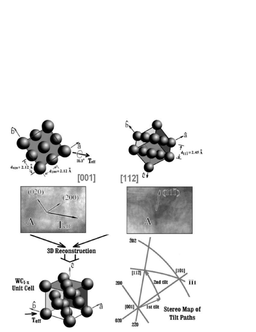
Figure 3: The tilt protocol for inferring the lattice structure of f.c.c. WC_1-x by viewing a WC_1-x crystal from its [001] zone and [112] zone, along which the two most easily resolved lattice plane sets, the {200} and {111} lattice planes, will show lattice fringes in HRTEM images. The two zones are 35.3^∘ apart, within the tilting limit of the microscope with a Gatan double tilt holder. The crystal is to be viewed along its [001] zone in the first specimen orientation, then tilted along the ($2\overline{2}0$) lattice planes to the [112] zone. The ($2\overline{2}0$) lattice planes must therefore be perpendicular to the effective tilt axis. The projections along the [001] and [112] zones together with the effective tilt axis have been drawn so that their azimuths are consistent with those in the 700K HRTEM images. The experimental HRTEM images of a WC_1-x nano-crystal acquired using this protocol and their power spectra are shown in the bottom. The actual tilt sequence is to tilt along -T₂ by 19.5^∘ followed by tilting along -T₁ by 30.0^∘, where T₁ and T₂ denote the side-entry goniometer tilt axis and the second tilt axis of a Gatan double tilt holder, respectively.

III.4 Double tilting

The specimen was first tilted about $T_{2}$ to $\vartheta_{2}=9.7^{\circ}$ while $\vartheta_{1}$ remained at $0^{\circ}$, made eucentric, then tilted about $T_{1}$ to $\vartheta_{1}=15.0^{\circ}$. The first HREM image was taken at this specimen orientation of ($\vartheta_{1}=15^{\circ}$,$\vartheta_{2}=9.7^{\circ}$). A similar sequence was applied to take a second HREM image at the second specimen orientation of ($\vartheta_{1}=-15^{\circ}$, $\vartheta_{2}=-9.7^{\circ}$). The process can be modeled with a simple matrix calculation Liu et al. (1989); Tambuyser (1985).

Because of the importance of repeatable quantitative tilts, effects of “mechanical hysterisis” were minimized by inferring all relative changes in tilt from goniometer readings taken with a common direction of goniometer rotation. The rotation sequences were “initialized” by first tilting past the starting line, and then returning to it in the direction of subsequent motion. Nonetheless both the precision of angle measurement, and our inability to observe lattice fringes during rotation, were shortcomings that microscopes designed to apply these strategies routinely must address.

III.5 Specimen preparation

The tungsten carbide thin film was deposited by PECVD on glass substrates by introducing a gaseous mixture of tungsten hexacarbonyl and hydrogen into a RF-induced plasma reactor at a substrate temperature of $330^{\circ}$C Qin et al. (1998). The specimen was disk-cut, abraded from the glass substrate side and dimpled by a Gatan Model 601 Disk Cutter, a South Bay Technology Model 900 Grinder and a Gatan Model 656 Precision Dimpler, respectively. The specimen was then argon ion-milled by a Gatan DuoMill for about 5 hours to perforation prior to the TEM study, at an incidence angle of $3^{\circ}$.

IV Experimental Results

IV.1 Diffraction from a known to check column geometry

Calibration of these algorithms with geometry in our microscope was first done with diffraction data from a Si crystal. Diffraction patterns of $\langle 100\rangle$ Si along the [$1\overline{1}\overline{6}$] and [$1\overline{1}6$] zone axes were obtained by tilting about $T_{1}$ and $T_{2}$. The lattice parameters determined are ($a=0.383$nm, $b=0.387$nm, $c=0.386$nm, $\alpha=60.0^{\circ}$, $\beta=119.6^{\circ}$, $\gamma=119.1^{\circ}$). This set of chosen basis defines the rhombohedral primitive cell of the Si f.c.c lattice. Compared with the literature values of Si ($a=0.384$nm, $b=0.384$nm, $c=0.384$nm, $\alpha=60^{\circ}$, $\beta=120^{\circ}$, $\gamma=120^{\circ}$), the angular disagreements are less than $1^{\circ}$ and spatial disagreements are less than $1\%$. These uncertainties are comparable to those obtained by other techniques of submicron crystal analysis Liu (1990); Liu et al. (1992, 1989); Tambuyser (1985); Fraundorf (1981b).

IV.2 Nanocrystal images to infer lattice parameters of an unknown

The micrographs in Figure 3 show a nanocrystal in a film rich in tungsten carbide, at the orientations of ($\vartheta_{1}=15^{\circ}$, $\vartheta_{2}=9.7^{\circ}$) and ($\vartheta_{1}=-15^{\circ}$, $\vartheta_{2}=-9.7^{\circ}$) respectively. The coordinates of periodicities in micrograph power spectra, as well as in the common reference coordinate system, are listed in Table 1, in much the same format as is diffraction data for stereo analysis Fraundorf (1981b).

Table 1: The g-spacings $[nm^{-1}]$ and azimuths $[^{\circ}]$ of three spots measured from the power spectra of images at two tilts, as well as calculated Cartesian coordinates $[nm^{-1}]$ of those reciprocal lattice spots in a common coordinate system. This constitutes a minimal data set for analyzing the lattice in three-dimensions.

Spot $n$	$g_{m}$	$\varphi_{m}$	$\vartheta_{1}$	$\vartheta_{2}$	$g_{x}$	$g_{y}$	$g_{z}$
1	4.73	79.2	-15.0	-9.7	0.861	4.53	-1.01
2	4.77	-11.6	-15.0	-9.7	4.52	-1.15	-1.03
3	4.14	32.6	+15.0	+9.7	3.37	2.04	1.27

IV.2.1 Matching the lattice:

The lattice spacings and inter-spot angles of periodicities in image power spectra were used to look for consistent indexing alternatives from a set of 36 tungsten carbide and oxide candidate lattices including WC_1-x. When an angular tolerance of $2^{\circ}$ and a spatial tolerance of $2\%$ are imposed, only WC_1-x provides a consistent indexing alternative. As summarized in Table 2, the Miller indices of the three observed spots then become ($200$), ($020$) and ($11\overline{1}$). The images of Figure 3 thus represent WC_1-x [001] and [112] zones, respectively. The azimuth of the reciprocal lattice vector ($2\overline{2}0$),

$$\varphi_{(2\overline{2}0)}=\frac{\left(\varphi_{(200)}+\left[180^{\circ}+\varphi_{(020)}\right]\right)}{2}=123.8^{\circ}\text{,}$$ (7)

deviates from the projection of the effective tilt axis by only $0.3^{\circ}$. Therefore the ($2\overline{2}0$) lattice planes are perpendicular to the effective tilt axis as per Figure 4, and the data acquired are consistent with the expectation for fcc crystals outlined in Figure 3. The actual tilting path in the Kikuchi map of crystal A is shown there as well.

Table 2: The results of a three-dimensional match of measured spacings $[nm]$ and interspot angles $[^{\circ}]$, with those predicted from the literature (denoted with a caret) for the face-centered cubic crystal WC_1-x. This phase is the only one from a list of 36 tungsten carbides and tungsten oxides whose predicted spacings and interspot angles agreed the measurements within a tolerance of $1.5\%$ and $1.5^{\circ}$, respectively.

Spot $n$	$d_{n}$	$\varphi_{ij\neq n}$	$(hkl)$	$\widehat{d_{hkl}}$	$\frac{\delta d}{d}[\%]$	$\widehat{\varphi_{ij\neq n}}$	$\delta\varphi$
1	0.212	54.2	($200$)	0.212	0.5	54.7	0.5
2	0.209	56.2	($020$)	0.212	1.4	54.7	1.5
3	0.242	90.8	($11\overline{1}$)	0.245	1.2	90.0	0.8

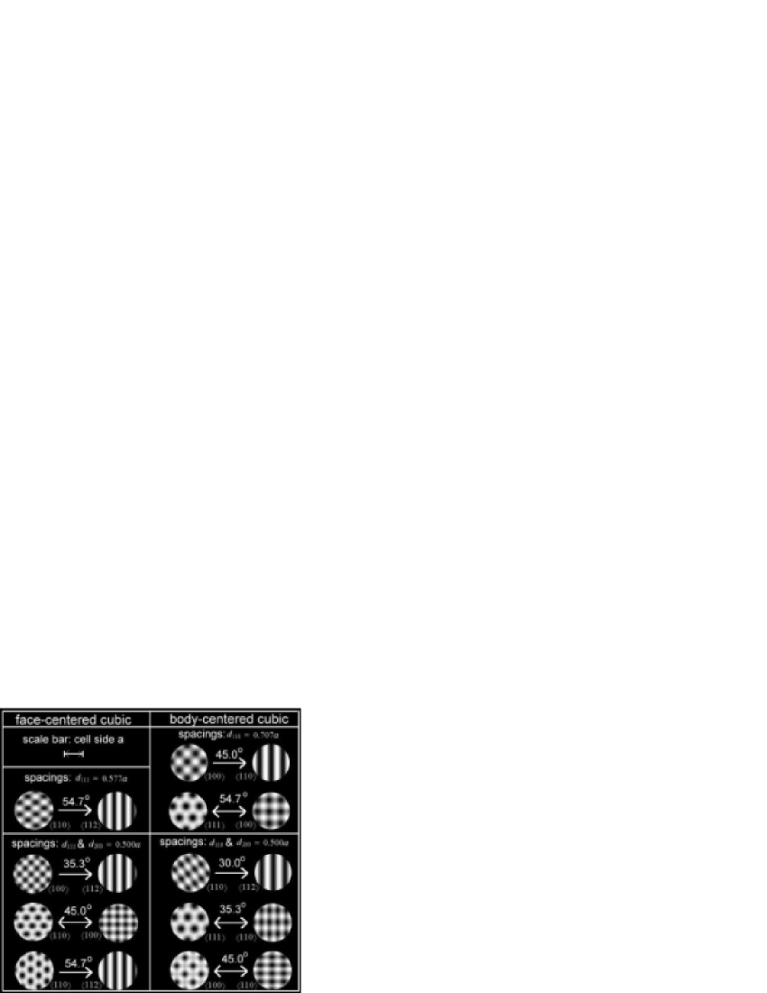
Figure 4: Illustration of all ways (from Figure 1) to verify the three dimensional lattice parameters of fcc and bcc crystals from a pair of lattice images, given an ability to image only lattice spacings down to half the unit cell side, and a tilt range of less than 60 degrees. The image pairs are rotated so as to illustrate the direction of tilt between the two zones (crystal orientations) involved. The protocols shown with double arrows provide access to cross-fringes (and hence information on which direction to tilt) at both ends of the tilt sequence. Also note that the first and last entries in each column simply provide low and high resolution views, respectively, of the same experiment.

From the indexing suggested by this match, the $x$, $y$, and $z$ coordinates of the reciprocal lattice basis vectors $a^{\ast}$, $b^{\ast}$, and $c^{\ast}$ may be inferred. This is shown in Table 3, along with the resulting lattice parameters and a comparison with literature values. The resulting errors in $a$ and $b$ are less than $1.3\%$, while the error in $c$ (which is orthogonal to the plane of the first image) is larger (around $2.3\%$). Both because of tilt uncertainties and reciprocal lattice broadening in the beam direction, uncertainties orthogonal to the plane of the specimen are expected to be larger than in-plane errors Fraundorf (1987).

Table 3: Primitive (top) and face-centered (bottom) reciprocal lattice basis triplets (spacings in nm, angles in degrees) inferred from our two HREM images of crystal A, along with a comparison of the lattice parameters for each cell which follow therefrom. The indexing of the observed reciprocal lattice vectors in these two cases was inferred directly for the primitive cell, by minimizing cell volume, and by matching to “textbook” parameters for WC_1-x in the case of the face-centered cell. Except for the choice of basis triplet, the two measured cells refer to exactly the same inferred lattice.

measured	0.298	0.299	0.296	120.0	58.7	119.8
“book”	0.300	0.300	0.300	120	60	120
params	$a$	$b$	$c$	$\alpha$	$\beta$	$\gamma$
“book”	0.425	0.425	0.425	90	90	90
measured	0.424	0.419	0.415	88.5	90.8	89.3

IV.2.2 Building a triplet from scratch:

By generating linear integral combinations of the measured periodicities in reciprocal space (i.e. vector triplets of the form $n_{1}g_{1}+n_{2}g_{2}+n_{3}g_{3}$ where the $n_{i}$ are integers) until a minimal volume unit cell is obtained (there will be more than one way to achieve the minimum), a primitive triplet for the measured lattice can be inferred quite independent of any knowledge of candidate lattices. The primitive cell parameters determined are also listed in Table 3. With respect to literature values, these show spatial disagreements of less than $1.6\%$, and angular disagreements of less than $1.5^{\circ}$. Although inference of the “conventional cell” from the primitive cell alone is possible, the process has not been attempted here because of complications attendant to measurement error.

IV.2.3 Phase Identification

Determining a reciprocal lattice triplet, and inferring lattice parameters therefrom, are of course not equivalent to confirming the existence of a particular phase. In order to draw a more robust conclusion about the makeup of crystal A, we extended our analysis of the structure to other lattices capable of indexing the observed spots, albeit with larger errors in spacing and interspot angle. When the spatial and angular tolerances of our candidate match analysis are increased to $3^{\circ}$ and $3\%$, there are many tungsten oxide and carbide candidates in addition to WC_1-x which show consistent lattice spacings and inter-planar angles Qin et al. (1998).

In order to eliminate these candidates, it was necessary to confirm, using power spectra of amorphous regions in each image, that the spatial frequencies in Figure 3images were continuously transferred within the first passband Spence (1988); Williams and Carter (1996). By then assuming that projected reciprocal lattice frequencies make their way into the exit surface wavefield (at least at the thin edges of the particle), all the candidates except WC_1-x are eliminated. Specifically, it was found that for each of the candidates except WC_1-x, along one or more of the suggested zone axes at least one reciprocal lattice vector shorter than the experimental one(s) is missing in a power spectrum Qin et al. (1998). An example of this is the match with hexagonal WC_x ($a=1.058$nm, $c=1.335$nm). In this case the Miller indices suggested for spot 3 ($\overline{4}2\overline{2}$) were inconsistent with the fact that the ($\overline{2}1\overline{1}$) is absent from the power spectrum of the image on the right side of Figure 3.

Our conclusion that “this crystal is WC_1-x” (and as we see later most of the other crystals in the specimen) is consistent with knowledge of the formation conditions, as well as with X-ray powder and EDS analysis of the same film.

IV.3 The effective tilt direction, and recurring fringes

In addition to serving as a guide for correctly choosing the azimuth of the crystal before tilting between desired zones, knowledge of the tilt axis direction plays another role: that of highlighting lattice fringes present in both specimen orientations, but caused by one and the same set of lattice planes.

In single tilt experiments, the tilt axis is simply $T_{1}$. This is always perpendicular to the electron beam and hence parallel to the micrographs. Any reciprocal lattice vector parallel or antiparallel to $T_{1}$ remains in Bragg condition throughout the whole tilting process, regardless of the amount of tilt $\vartheta_{1}$. If the spacing is large enough to be recorded in the images, the same lattice fringes are seen perpendicular to the projection of $T_{1}$ in any HREM image as well.

For double tilt experiments, it is convenient to introduce the concept of an effective tilt axis. The effective tilt axis is analogous to the tilt axis in a single tilt experiment, in that the double tilt can be characterized by a single tilt around the effective tilt axis of angular size equal to that in the double tilt. This effective axis is perpendicular to the electron beam and hence parallel to the micrographs only if the two specimen orientations are symmetric about the untilted position.

Considering only double tilts falling into this category, let ($\vartheta_{1}$, $\vartheta_{2}$) and ($-\vartheta_{1}$, $-\vartheta_{2}$) denote the specimen orientations before and after. The effective tilt axis direction has an azimuth (with respect to our reference $x$-direction) of

$$\varphi_{eff}=\tan^{-1}\left[-\frac{\sin(\vartheta_{1})}{\tan(\vartheta_{2})}\right]\text{.}$$ (8)

A proof of equation 8 is given in Appendix A. There exists a 180^∘ ambiguity in the direction of the effective tilt axis using equation 8. This ambiguity can be resolved through the knowledge of the actual tilting sequence. In our experiment $\vartheta_{1}=15^{\circ}$, $\vartheta_{2}=9.7^{\circ}$, $\varphi_{eff}=123.5^{\circ}$. This is the effective tilt axis direction mentioned in previous sections.

Lattice planes perpendicular to the effective tilt axis, in the double tilt case, diffract and are visible at initial and final, but not intermediate, specimen orientations. This result inspired further experimental work on, and modeling of, fringe visibility loss during tilt Qin (2000). One result of this exercise was a prediction that $0.213$nm fringes deviating by as much as $4^{\circ}$ from the effective tilt direction in a 10nm $WC_{1-x}$ specimen will remain visible after a $35.6^{\circ}$ tilt. This was confirmed by experiment on these specimens Qin (2000). The result in turn serves to constrain the probability and error analyses below.

IV.4 Tilt limitations and chances for success

This section addresses the chances for successful 3D cell determination from images, depending on properties of both microscope and specimen. Such matters are considered in more detail elsewhere Qin (2000).

In a microscope with a single-axis tilt of at least $\pm 35.3^{\circ}$ and a stage capable also of $180^{\circ}$ rotation, any cubic crystal with an [$001$] zone in the beam direction at zero tilt can be re-aligned by azimuthal rotation until its ($2\overline{2}0$) reciprocal lattice vector is parallel to T₁. With an untilted tilt-rotate stage, this would allow a crystal’s [$001$] zone to remain aligned with the beam throughout the rotation. Subsequent tilting by $35.3^{\circ}$ will lead to the [$112$] zone, and the lattice structure in three dimensions confirmed ala Figure 3.

Under these conditions, any cubic crystal showing [$001$] zone cross fringes can be tilted so as to reveal a third spacing. Hence the probability of success with any given crystal is that of finding a randomly-oriented crystal oriented with [$001$]-zone fringes visible. Fortunately for this method, the spreading of reciprocal lattice points due to finite crystal thickness $t$ allows one to visualize fringes within a half angle $\Theta_{t}$ of order $1/t$ surrounding the exact Bragg condition. Otherwise, cross-fringes would be rare indeed!

The solid angle subtended by this visibility range for lattice planes intersecting along the [$001$]-zone allows us to calculate the probability that a randomly-oriented crystal will show cross-fringes of specified type. For example if we approximate the cross-fringe region with a conical bundle of directions about each zone, then for the special case of spherical particles the fraction of crystals showing the fringes of zone $x$ is:

$$p_{x}=n(1-\cos[\Theta_{t}])\text{, where }\Theta_{t}=\arcsin[\frac{g_{t}^{2}-g_{x}^{2}+2g_{\lambda}g_{t}}{\sqrt{2}g_{x}g_{\lambda}}]\text{,}$$

$n$ is multiplicity of zone $x$ (e.g. $n=3$ for cubic $x=$[$001$]), $g_{x}=1/d$, $g_{\lambda}=1/\lambda$, and $g_{t}=f/t$, where $t$ is the thickness of the crystal in the direction of the beam and $f$ is a parameter of order one that empirically accounts for signal-to-noise in the method used to “visualize” fringes. For example, we expect $f$ to decrease if an amorphous film is superimposed on the crystals being imaged. The half-angle $\Theta_{t}$ is a pivotal quantity in both the probability and accuracy of fringe measurement.

A plot of the probability for seeing [$001$] cross-fringes of spacing $d=0.202$nm, as a function of specimen thickness $t$ for both spherical and laterally-infinite (rel-rod) particles, is shown in Fig. 5. Here we’ve used fit parameter $f=0.79$ based on data points (also plotted) that were obtained experimentally for particles of varying size from HREM images of Au/Pd evaporated onto a carbon film. As you can see, the probability of encountering cross-fringes improves greatly as crystallite size decreases toward a nanometer. Of course, as discussed in the next section, this “reciprocal lattice broadening” is accompanied by a decrease in the precision of measurements for individual lattices.

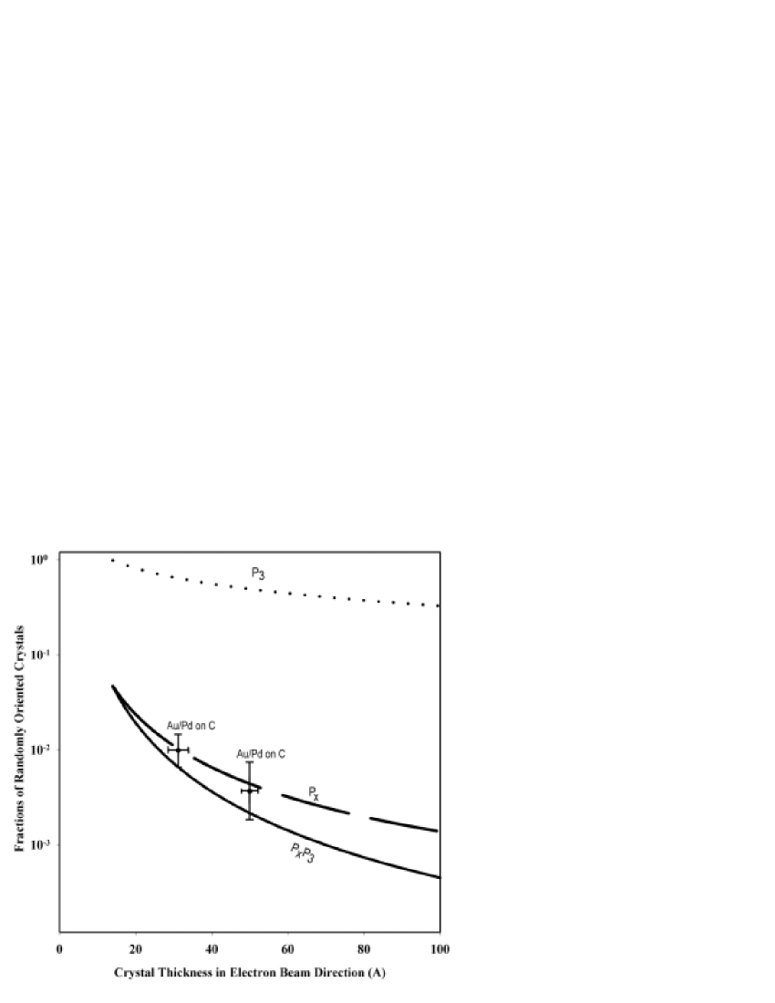
Figure 5: A plot of the fraction of randomly oriented grains of WC_1-x showing [001]-zone cross fringes ($p_{x}$), and the fraction of such cross-fringe grains oriented so that a random tilt of 35.3 ^∘ will allow imaging of a 111 periodicity ($p_{3}$), as a function of specimen thickness in the direction of the electron beam. Qin and Fraundorf (2000)

Due to the tilt limits of the specimen holder in our microscope, the first HREM image along the [$001$] zone of a WC_1-x nano-crystal had to be taken at a nonzero $\vartheta_{1}$ orientation. Azimuthal symmetry is thus broken. Our solution was to find a [$001$] nano-crystal whose ($2\overline{2}0$) reciprocal lattice vector was by chance parallel to the effective tilt axis, then tilting to the 2nd orientation. Thus nano-crystal $A$ was identified (by coincidence) to have an appropriate azimuth during real time study of the ($200$) and ($020$) lattice fringes. Tilting by $35.3^{\circ}$ was done thereafter.

For the probability of success in our case, we must multiply $p_{x}$ by the probability of viewing ($111$) fringes after tilting a [$001$] crystal with random aziumth by $35.26^{\circ}$. This probability of finding a 3rd spacing takes the form $p_{3}=m\delta/\pi$, where $m$ is the multiplicity of target spacings (e.g. $m=4$ for a four-fold symmetric [$001$] starting zone), and the “azimuthal tolerance half-angle” $\delta$ (again in the spherical particle case) obeys the implicit relation:

$$\theta_{o}=\arctan[\frac{\tan\theta_{o}}{\cos\delta}]+\arctan[\frac{\cos\gamma}{\sin^{2}\gamma-(\cos\theta_{o}\sin\delta)^{2}}]\text{,}$$

where $\theta_{o}$ is the required tilt (in our case $35.26^{\circ}$) and

$$\gamma=\arccos[\frac{g_{d}^{2}-g_{l}^{2}-2g_{\lambda}g_{l}}{2g_{d}g_{\lambda}}]\text{.}$$

The probability $p_{3}$ is also plotted as a function of specimen thickness in Fig. 5, along with the product $p_{x}p_{3}$.

These models predict a probability of success with the strategy adopted in our experiment, for the “large” $10$nm WC_1-x crystals in our specimen, of $p_{x}p_{3}=7.3\times 10^{-4}\times 0.371=2.4\times 10^{-4}$. Hence only one in every $1500$ crystals will show [$001$] cross fringes, and one in every $4000$ will be suitably oriented for 3D lattice parameter determination. This is consistent with our experience: The image of crystal A was recorded in one negative out of 22, each of which provided an unobstructed view of approximately $100$ crystals.

As mentioned above, using a microscope capable of side-entry goniometer tilting by $\pm 35.3^{\circ}$ with a tilt-rotate stage, the 3D parameters of all cubic crystals, when untilted showing [$001$] zone cross-fringes, could have been determined. According to Fig. 14a, the fraction of particles $2$ nm in thickness that are oriented suitably for such analysis approaches $1$ in $100$. Moreover, with a goniometer capable of tilting by $\pm 45^{\circ}$ plus computer support for automated tilt/rotation from any starting point, each unobstructed nano-crystal in the specimen could have been subjected to this same analysis after a trial-and-error search for accessible [$001$] zones. Thus a significant fraction of crystals in a specimen become accessible to these techniques, with either a sufficient range of precise computer-supported tilts, or if the crystals are sufficiently thin.

Subsequent work Fraundorf and Qin (2001) has shown that information on tilt protocols and fringe visibility for crystals of a given thickness can be elegantly sumarized with spherical maps like those in Figure 6. These are a direct-space analog to reciprocal-space Kikuchi maps, in which band thickness is proportional to d (rather than 1/d). If the sphere used has a diameter equal to specimen thickness, then the first order effect of changing thickness simply increases the separation between zones while holding the width of the bands fixed.

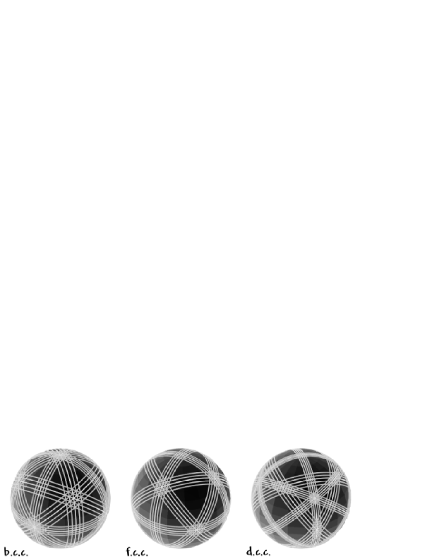
Figure 6: Visibility maps for the two largest fringes visible from body-centered, face-centered, and diamond face-centered lattices. Sphere diameter (relative to band width and fringe spacing) is proportional to specimen thickness, here chosen to be about 5 times the cubic cell side a. Note the dominance of crossed $(110)$ fringes at the three-fold $\langle 111\rangle$ zone in the body-centered case, the dominant crossed $(111)$ fringes at the two-fold $\langle 110\rangle$ zone in the face-centered cases, and the wider disparity between largest and next-to-largest spacings when the diamond glide is added to the lattice.

V Pitfalls and uncertainties

V.1 Cautions involving specimens and contrast transfer

In this section, we discuss effects warranting caution. In the next section, models of lattice parameter uncertainty are discussed.

High electron beam intensities can cause lattice rearrangement in sufficiently small nanocrystals, as well as changes in the orientation of a thin film (e.g. due to differential expansion). Sequential images of the same region at fixed tilt might allow one to check for such specimen alterations.

Loss of periodicities in the recorded image, due to damping and spherical aberration zeros, were discussed in the section above on experimental design. Nonetheless, careful observations of more than one crystal, and image simulation as well, may be useful adjuncts whenever this technique is applied. We illustrate this below, with a “two-dimensional” experiment done to assess the size of errors due to finite crystal size and random orientation. The result is of help in the section on modeling uncertainties that follows.

A recent paper on HREM image simulations Malm and O’Keefe (1997) indicated that deviations in orientation of a 2.8nm spherical palladium nano-crystal from the zone axes may result in fringes unrelated to the structure of the particle. Variability in measured lattice spacings was also reported to be as high as several percent, with the highest reaching 10%. To compare such results with our experimental data, 23 single crystals free of overlap with other crystals, and each showing cross-fringes, were examined. The projected sizes of these crystals range from 3.7nm$\times$3.8nm to 10.8nm$\times$7.8nm. The spacings and angles between fringes are plotted in Fig. 7.

Observed cross-fringes in the HREM images fall into two categories, according to their spacings and angles. The first category is characterized by a $90^{\circ}$ inter-planar angle between two $2.12\AA$ lattice spacings. The second one by two inter-planar angles of $55^{\circ}$, $70^{\circ}$ and three lattice spacings of $2.12\AA$, $2.12\AA$, $2.44\AA$. Only the spacings of $2.44\AA$ and $2.12\AA$ and the corresponding angle of $55^{\circ}$ have been shown in Figure 7. Two conclusions can be drawn.

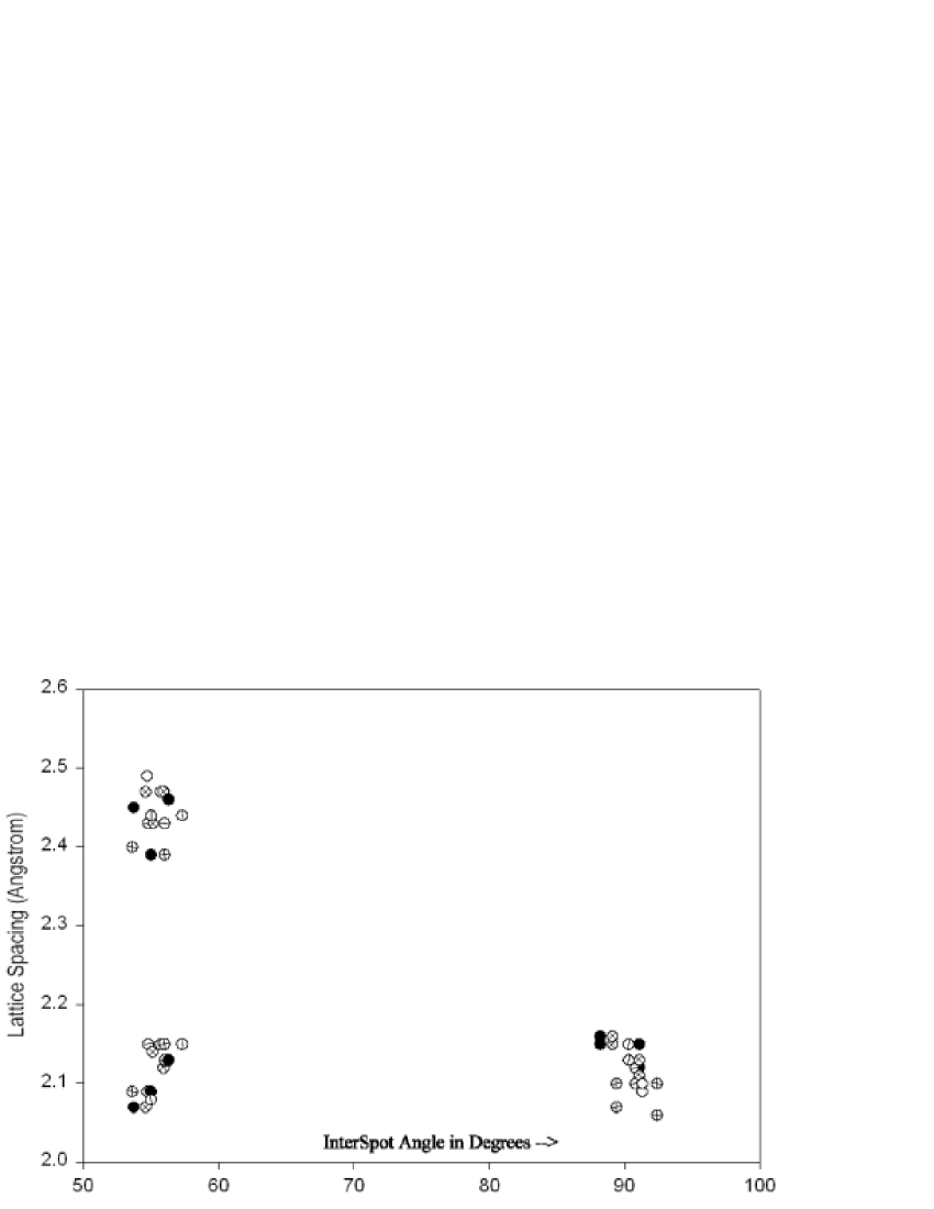
Figure 7: The spacings and interplanar angles measured from the cross lattice fringes of 23 nano-crystals free of overlap with other crystals in the HRTEM images. Insets (b) and (c) are magnified plots of the two regions in (a) where all the data are concentrated. The specific combinations of lattice spacings and interplanar angles corresponds to the [001] and [011] zone images of WC_1-x and hence indicate WC_1-x being the only present phase in the thin film. The measured lattice spacings have a standard deviation from their mean of less than 1.5%, and interplanar angles have a standard deviation of 1.2^∘.

First, since the two categories of cross-fringes match those along the [$001$] and [$011$] zone axes of WC_1-x, the only two zones which show cross-lattice fringes in our HREM images, the thin film consists mainly of WC_1-x. X-ray powder diffraction work on the film supports this conclusion Qin et al. (1998).

Secondly, for nano-crystals free of overlap with other crystals, the observed lattice spacings and interplanar angles in HREM images have a standard deviation from the mean of less than $1.5\%$, and a standard deviation of less than $1.3^{\circ}$, respectively. We have not observed any seriously shortened or bent fringes. Nonetheless we recommend that such fringe abundance analyses go hand in hand with stereo lattice studies of nano-crystal specimens, and that comparative image simulation studies be done where possible as well.

V.2 Uncertainty forecasts

Earlier estimates Fraundorf (1987), as well as the typical size of diffraction broadening in the TEM, suggest that lattice parameter spacing errors may in favorable circumstances be on the order $1\%$, and angle errors on the order of $1^{\circ}$. Experiment, and a more detailed look at the theory Qin (2000), now support this impression. We will focus the discussion here on equant or spherical nanocrystals. The results should be correct within $10\%$ for other (e.g. thin-foil) geometries of the same thickness.

The three sources contributing to the lattice spacing measurement uncertainty in images are: expansion of the reciprocal lattice spot in the image plane, uncertainty in the camera constant, and expansion of the reciprocal lattice spot along the electron beam direction, in order of decreasing relative effect Qin (2000). The uncertainty in our camera constant is measured to be about $0.5\%$. Uncertainties from the first and third sources above are on the order of $1\%$ and $0.01\%$, respectively, for a typical lattice spacing of 0.2 nm. The in-plane/out-of-plane error ratio is on the order of 10.

Sources contributing to the measurement uncertainty of lattice parameters along the electron beam direction, when the specimen is un-tilted, include uncertainty in goniometer tilt as well as sources analogous to those above. Observation of reciprocal lattice vectors further out of the specimen plane (i.e. of fringes at high tilt) reduces the measurement uncertainty of “out-of-plane” parameters.  The measurement uncertainty of inter-planar angles in images is due to lateral uncertainty in their associated reciprocal lattice spots in the image plane.

Using a mathematical model of these errors Qin (2000), we predict spacing uncertainties in a 10 nm nanocrystal, tilted by $\pm 18^{\circ}$, of $2.1\%$ for an imaged spacing and of $8.6\%$ for a lattice parameter perpendicular to the plane of the untilted specimen. This large “out-of-plane” uncertainty is a result of the small tilt range available with our high resolution pole piece. The estimated interplanar angle uncertainty is about $2.3^{\circ}$. These predicted uncertainties Qin (2000) are between 2 and 3 times the errors observed here, and hence of the right order of magnitude.

The model suggests that lattice parameter uncertainties will decrease as camera constant and tilt uncertainties decrease, and will also decrease as the tilt range used for the measurement increases. It suggests that the lattice parameter errors will increase as crystal thickness goes down. The ease of locating spacings, however, goes up as crystal thickness decreases. Hence the best candidates for application of the protocols here may be crystals in the 1 to 20 nm range. Improved tilt accuracy (hopefully with computer guidance), and low-vibration tilting so that fringes may be detected as orientation changes, would make these strategies more accurate and widely applicable as well.

VI Conclusions

When considered from the perspective of direct space imaging, crystals offer a discrete set of opportunities for measuring their lattice parameters in three dimensions. Ennumerating those opportunities for candidate lattices, or lattice classes, opens doors to the direct experimental determination of nano-crystal lattice parameters in 3D. A method for doing this, and lists of those opportunities for the special case of cubic crystals, are presented here.

We apply this insight to inferring the 3D lattice of a single crystal from electron phase or Z-contrast images taken at two different orientations. For nano-crystals in particular, a double-axis tilt range of $\pm 18^{\circ}$ degrees allows one to get such data from all correctly-oriented cubic crystals with appropriate spacings resolvable in a pair of images taken from directions separated by $35.3^{\circ}$. In the experimental example presented, we find less than $1.5\%$ spatial and $1.6^{\circ}$ angular disagreements between the inferred primitive cell lattice parameters of a 10 nm WC_1-x nano-crystal, and literature values.

We further present data on the variability of lattice fringe spacings measured from images of such randomly-oriented 10nm WC_1-x crystals in electron phase contrast images. The results suggest that measurement accuracies of $2\%$ in spacing and $2^{\circ}$ in angle may be attainable routinely from particles in this size range. Smaller size crystals may be easier to obtain data from, but show larger uncertainties, while larger or non-randomly oriented crystals (especially if guesses as to their structure are unavailable) may be more challenging to characterize in three dimensions.

Precise knowledge of the tilt axes, as projected on the plane of a micrograph, is crucial to implementation. This information, if coupled with on-line guidance on how to tilt from an arbitrary two-axis goniometer orientation in any desired direction with respect to the plane of an image or diffraction pattern, could make this strategy and related diffraction strategies Fraundorf (1981b) for lattice parameter measurement more routine. Future microscopists might then be able to interface to individual nanocrystals much as the nano-geologist in the first paragraph of this paper examined her “hand specimen”.

Lastly, diffraction can also be used in this “stereo analysis” mode (with crystals large enough to provide diffraction patterns), although the easier accessibility of high spatial frequencies via diffraction often makes the large tilts used here unnecessary. They can also be put to use in darkfield imaging applications, by forming images of the specimen using “beams” diffracted by the periodicities which serve as diagnostic of a given lattice (for example those associated with each of the protocols of Figure 1).

Images so taken of nano-crystalline specimens, for example at two tilts with three different darkfield conditions, would be expected to show correlations among that subset of the crystals correctly oriented for diffraction with all three reflections. Although this strategy may never allow precise lattice parameter determinations given limits on objective aperature angular size, it may be a very efficient way to search for crystals correctly-oriented and of correct type for one of the imaging protocols described here. Moreover, because such lattice-correlations in three dimensions contain information beyond the pair-correlation function, they may be able to support the new technique of fluctuation microscopy Treacy and Gibson (1993, 1996); Voyles et al. (2000) in the study of paracrystalline specimens like evaporated silicon and germanium Gibson and Treacy (1997, 1998) whose order-range is too small for detection by other techniques.

Appendix A Effective tilt axis azimuth

Let ($\vartheta_{1}$, $\vartheta_{2}$) and ($\vartheta_{1}^{\prime}$, $\vartheta_{2}^{\prime}$) denote orthogonal tilt values for two specimen orientations, and $\phi_{eff}$ the azimuth of the effective tilt axis between these orientations. Any reciprocal lattice vector with untilted Cartesian coordinates $|g\rangle$, and with identical micrograph coordinates $|g_{m}\rangle$ at the two tilted orientations, will (following equation 4) obey:

$$A(\vartheta_{1},\vartheta_{2})|g_{m}\rangle=|g\rangle=A(\vartheta_{1}^{\prime},\vartheta_{2}^{\prime})|g_{m}\rangle\text{,}$$ (9)

where

$$|g_{m}\rangle=\left(\begin{array}[]{c}g\cos\left(\varphi_{eff}\right)\\ g\sin\left(\varphi_{eff}\right)\\ 0\end{array}\right)\text{.}$$ (10)

Expanding, this gives three equations which, combined with equation 10 $g_{mx}=g_{my}\tan(\varphi_{eff})$, can be solved for the three unknowns $\vartheta_{1}^{\prime}$, $\vartheta_{2}^{\prime}$, $\varphi_{eff}$, to get:

$$\vartheta_{1}^{\prime}=-\vartheta_{1}\text{, }\vartheta_{2}^{\prime}=-\vartheta_{2}\text{, and}$$ (11)

$$\varphi_{eff}=\tan^{-1}\left[-\frac{\sin(\vartheta_{1})}{\tan(\vartheta_{2})}\right]\text{.}$$ (12)

This provides an equation for the azimuth of the effective tilt, and confirms that symmetry about the zero tilt position is a necessary and sufficient condition for the reciprocal lattice vector $|g\rangle$, and it’s associated lattice fringe, to show a common direction in micrographs at both tilts.