[

The number of guards needed by a museum: a phase transition in vertex covering of random graphs

Abstract

In this letter we study the NP-complete vertex cover problem on finite connectivity random graphs. When the allowed size of the cover set is decreased, a discontinuous transition in solvability and typical-case complexity occurs. This transition is characterized by means of exact numerical simulations as well as by analytical replica calculations. The replica symmetric phase diagram is in excellent agreement with numerical findings up to average connectivity $e$, where replica symmetry becomes locally unstable.
Keywords (PACS-codes): General studies of phase transitions (64.60.-i), Classical statistical mechanics (05.20.-y), Combinatorics (02.10.Eb)

]

Imagine you are director of an open-air museum situated in a large park with numerous paths. You want to put guards on crossroads to observe every path, but in order to economize costs you have to use as few guards as possible. Let $N$ be the number of crossroads, $X<N$ the number of guards you are able to pay. Then there are $N\choose X$ possibilities of putting the guards, but the most “configurations” will lead to unobserved paths. Deciding whether there exists any perfect solution or finding one can thus take a time growing exponentially with $N$. In fact, this problem is one of the six basic NP-complete problems [1], namely vertex cover (VC). It is widely believed that no algorithm can be found which solves our problem substantially faster than exhaustive search for any configuration of the paths.

Similar combinatorial decision problems have been found to show interesting phase transition phenomena. These occur in their solvability and, even more surprisingly, in their typical-case algorithmic complexity, i.e. the dependence of the median solution time on the system size [2]. E.g. in satisfiability (SAT) problems a number of Boolean variables has to simultaneously satisfy many logical clauses. When the number of these (randomly chosen) clauses exceeds a certain threshold, the solvability of the full problem undergoes a sharp transition from almost always satisfiable to almost always unsatisfiable [3]. The instances which are hardest to solve are found in the vicinity of the transition point. Far away from this point the solution time is much smaller, as a formula is either easily fulfilled or hopelessly over-constrained. The typical solution times in the under-constrained phase are even found to depend only polynomially on the system size. Recently, insight coming from a statistical mechanics perspective on these problems [4] has lead to a fruitful cooperation with computer scientists, and has shed some light on the nature of this transition [5]. Frequently, the methods of statistical mechanics allow to obtain more insight than the classical tools of computer science or discrete mathematics.

This is also true for the above mentioned VC problem. After having introduced the VC model and reviewed some previously known rigorous results, we present numerical evidence for the existence of a phase transition in its solvability which is connected to an exponential peak in the typical case complexity. Due to the much simpler geometrical structure, many features of this transition can be understood much more intuitively than for SAT. In addition, we will see that the replica-symmetric [6] theory correctly describes the phase transition up to an average connectivity $e$. This is a fundamental difference to previously studied models with discontinuous transitions; see [7] for the example of 3-satisfiability where replica symmetry breaking is necessary to calculate the transition threshold.

Let us reformulate our problem in a mathematical way: Take any graph $G=(V,E)$ with $N$ vertices $i\in V=\{1,2,...,N\}$ (the crossroads in the above example) and edges $(i,j)\in E\subset V\times V$ (the paths). We consider undirected graphs, so with $(i,j)\in E$ we also have $(j,i)\in E$. A vertex cover is a subset $V_{vc}\subset V$ of vertices such that for all edges $(i,j)\in E$ there is at least one of its endpoints $i$ or $j$ in $V_{vc}$ (the path is observed). We call the vertices in $V_{vc}$ covered, whereas the vertices in its complement $V\setminus V_{vc}$ are called uncovered. Please note that the VC of a disconnected graph is consequently given by the union of the VCs of its connected components.

Also partial VCs $U\subset V$ are considered, where there are some uncovered edges $(i,j)$ with $i\notin U$ and $j\notin U$. The task of finding the minimum number of uncovered edges for given graph $G$ and the cardinality $|U|\equiv X$ is an optimization problem. We have already mentioned that the corresponding decision problem if a VC of fixed cardinality $X$ does exist or not, belongs to the basic NP-complete problems.

In order to be able to speak of typical or average cases, we have to introduce some probability distribution over graphs. We investigate random graphs $G_{N,c/N}$ with $N$ vertices and edges $(i,j)$ (with $i\neq j$) which are drawn randomly and independently with probability $c/N$. Thus the expected edge number equals ${N\choose 2}c/N=cN/2+O(1)$. The average connectivity $c$ remains finite in the limit $N\to\infty$ of infinitely large graphs. For $c<1$, these graphs are known to be decomposed into $O(N)$ connected components of typical size $O(1)$, whereas for $c>1$ a giant component appears which unifies $O(N)$ vertices [8]. For a more recent and complete introduction see [9].

As an element of a VC $V_{vc}$ typically covers $O(c)$ edges, the minimal cover size $X_{min}$ is also expected to be of $O(N)$, $X_{min}=x_{N,c}N$. In fact, there are rigorous lower and upper bounds on $x_{N,c}$ which are valid for almost all random graphs. To our knowledge, the best bounds are given in [10, 11], see Fig. 3 for a comparison with our results. The exact asymptotics for large connectivities $c\gg 1$ is also known, Frieze proved that [12]

$$x_{N,c}=1-\frac{2}{c}(\log c-\log\log c-\log 2+1)+o(\frac{1}{c})$$ (1)

for almost all graphs $G_{N,c/N},\ N\to\infty$.

It is however not clear, if a sharp threshold $x_{c}(c)=\lim_{N\to\infty}\overline{x_{N,c}}$ does exist at finite $c$, with the over-bar denoting the average over the random graph ensemble at fixed $N$ and $c$. In order to get some intuition on this point we have started our work with exact numerical simulations. Analytic results are presented below.

Using an exact branch-and-bound algorithm [13, 14] all optimal configurations at fixed $X$ are enumerated: As each vertex is either covered or uncovered, there are ${N\choose X}$ possible configurations which can be arranged as leaves of a binary (backtracking) tree. At each node of the tree, the two subtrees represent the subproblems where the corresponding vertex is either covered or uncovered. A subtree will be omitted if its leaves can be proven to contain less covered edges than the best of all previously considered configurations. The order of the vertices within the levels of the tree is given by their current connectivity, i.e. only neighbors are counted which are not yet included into the cover set. Thus, the first descent into the tree is equivalent to the greedy heuristic which iteratively covers vertices by always taking the vertex with the highest current connectivity.

First results are exposed in Fig. 1: The probability of finding a vertex cover of size $xN$ in a random graph $G_{N,c/N}$ is displayed for $c=2$ and several values of $N$, analogous results have been obtained for other values of $c$. The drop of the probability from one for large cover sizes to zero for small cover sets obviously sharpens with $N$, so that a jump at a well-defined $x_{c}(c)$ is to be expected in the large-$N$ limit: for $x>x_{c}(c)$ almost all random graphs with $cN$ edges are coverable with $xN$ vertices, below $x_{c}(c)$ almost no graphs have such a VC. Fig. 1 also shows the minimal fraction $e$ of uncovered edges as a function of $x$ for the partial covers. It vanishes for $x>x_{c}(c)$, whereas it remains positive for $x<x_{c}(c)$.

It is also interesting to measure the median computational effort, as given by the number of visited nodes in the backtracking tree, in dependence on $x$ and $N$. The curves, which are given in Fig. 2, show a pronounced peak near the threshold value. Inside the coverable phase, $x>x_{c}(c)$, the computational cost is growing only linearly with $N$, and in many cases the greedy heuristic is already able to cover all edges by covering $xN$ vertices. Below the threshold, $x<x_{c}(c)$, the computational effort is clearly exponential in $N$, but becomes smaller and smaller if we go away from the threshold. This easy-hard-easy scenario resembles very much the typical-case complexity pattern of 3SAT [5], and deserves some analytical investigation.

To achieve this, we use the strong similarity between combinatorial optimization problems and statistical mechanics. In the first case, a cost function depending on many discrete variables has to be minimized, e.g. the number of uncovered edges is such a cost function for vertex cover. This is equivalent to zero temperature statistical mechanics, where the Gibbs weight is completely concentrated in the ground states of the Hamiltonian. As the local variables for VC are binary because a vertex is either covered or uncovered, we may give a canonical one-to-one mapping of the vertex cover problem to an Ising model: for any subset $U\subset V$ we set $S_{i}=+1$ if $i\in U$, and $S_{i}=-1$ if $i\notin U$. The edges are encoded in the adjacency matrix $(J_{ij})$: an entry equals 1 iff $(i,j)\in E$, and $J_{ij}=0$ else. $(J_{ij})$ is thus a symmetric random matrix with independently and identically distributed entries in its lower triangle. The Hamiltonian, or cost function, of the system counts the number of edges which are not covered by the elements of $U$,

$$H=\sum_{i<j}J_{ij}\delta_{S_{i},-1}\delta_{S_{j},-1},$$ (2)

and has to be minimized under the constraint $|U|=xN$, which, in terms of Ising spins, reads

$$\frac{1}{N}\sum_{i}S_{i}=2x-1.$$ (3)

The resulting ground state energy $e_{gs}(c,x)$ equals zero iff the graph is coverable with $xN$ vertices.

We want to skip the details of the calculation, as these go beyond the scope of this letter. A detailed technical description will be presented elsewhere [16]. We only mention the main steps:
(i) We introduce a positive formal temperature $T$ and calculate the canonical partition function $Z=\sum_{{\cal{C}}_{x}}\exp\{-H/T\}$ where the sum is over all configurations $\{S_{i}\}_{i=1,...,N}$ which satisfy (3).
(ii) We are interested in the disorder-averaged free-energy density $f(c,x)=-\lim_{N\to\infty}TN^{-1}\overline{\ln Z}$, which we calculate using the replica method, closely following the scheme proposed in [15]. Within the replica symmetric framework, this free energy self-consistently depends on the order parameter $P(m)$ which is the histogram of local magnetizations $m_{i}=\langle S_{i}\rangle$. $\langle\cdot\rangle$ denotes the thermodynamic average.
(iii) The ground states are recovered by sending $T\to 0$. In this limit, one has to take care of the scaling of the order parameter with $T$, which is different below and above $x_{c}(c)$. For a similar reasoning in the case of 3SAT see also [7].
(iv) Both equations for $x<x_{c}(c)$ and $x>x_{c}(c)$ tend to the same limit for $x\to x_{c}(c)$. At the threshold, the resulting self-consistency equation can be solved analytically.

From this solution, many properties of the threshold VCs can be read off. The first is of course the value of the threshold itself:

$$x_{c}(c)=1-\frac{2W(c)+W(c)^{2}}{2c}$$ (4)

with the Lambert-W-function $W$ [17]. The result for $x_{c}(c)$ is displayed in Fig. 3 along with numerical data obtained by a variant of the branch-and-bound algorithm. For relatively small connectivities $c$ perfect agreement is found. We also have compared (4) with rigorous bounds obtained from counting VCs for small connected components having up to 7 vertices, which are very precise for small c (e.g. 0.999997N vertices are taken into account for c=0.1). Also here, perfect coincidence was found.

For larger $c$ systematic deviations of (4) from numerical results occur, it even violates the asymptotic form (1). For $c>e$, the replica symmetric solution becomes instable, and we find a continuous appearance of a replica symmetry broken solution; work is in progress on this point [16]. We conjecture, that the replica symmetric result (4) is exact for $c\leq e$, whereas it gives a lower bound for $c>e$ [18]. Please note that this point is situated well beyond $c=1$ where the giant component appears. Neither analytically nor numerically, we have found any influence of the giant component on the vertex covers. This is significantly different from Ising models on random graphs as studied in [19].

Besides the value of $x_{c}(c)$, the replica symmetric solution also contains structural information. One important phenomenon is a partial freezing of degrees of freedom. For a given random graph, there exists typically an exponential number of minimal VCs, thus the entropy density is finite. On the other hand, a fraction $b_{+}(c)$ of the vertices will be covered in all minimal VCs, thus forming a covered backbone, other vertices will never be covered and are collected in the uncovered backbone which has size $b_{-}(c)N$:

$$b_{-}(c) = \frac{W(c)}{c}$$ (5)

$$b_{+}(c) = 1-\frac{W(c)+W(c)^{2}}{c}$$ (6)

In Fig. 3 the total backbone size $b_{c}(c)=b_{-}(c)+b_{+}(c)$ is compared with numerical data, again very good agreement is found in the range of validity of replica symmetry.

For small $c$, the uncovered backbone is large, which is mainly due to isolated vertices which have to be uncovered in minimal VCs. The simplest structure showing a covered backbone are subgraphs with three vertices and two edges. In the minimal VC of this subgraph, the central vertex is covered, thus belonging to the covered backbone, the other two are uncovered, thus belonging to the uncovered backbone. The simplest non-backbone structures are components with only two vertices and one edge, because the vertices have no unique covering state.

These backbones appear discontinuously at the threshold because inside the coverable phase the backbone is empty. The proof is simple ($x>x_{c}(c)$ fixed):
(i) Assume that there is a non-empty uncovered backbone, with $i$ being an element. Now take any minimal cover $V_{0}$. It can be extended by covering arbitrarily chosen $(x-x_{c}(c))N$ vertices out of $V\setminus V_{0}$, e.g. vertex $i$, which is a contradiction to our assumption.
(ii) Assume now a non-empty covered backbone, with $i$ being an element. Then $i$ has to be an element of $V_{0}$. As the connectivity of $i$ is almost surely smaller than or equal to $O(\log N)$, all uncovered neighbors of $i$ can be covered by some of the $(x-x_{c}(c))N$ covering marks (for $N$ sufficiently large), and $i$ can be uncovered without uncovering the graph. This is again a contradiction to our assumption.

To summarize, we have investigated the vertex cover problem on random graphs by means of exact numerical simulations and analytical replica calculations. A sharp transition from a coverable to an uncoverable phase is found by decreasing the permitted size of the cover set. This transition coincides with a change of the typical case complexity from linear to exponential growth in $N$ and the discontinuous appearance of a frozen-in backbone. The complete RS solution was given for $c<e$, it is found to be in perfect agreement with numerical results. For $c>e$ the behavior is less clear as replica symmetry breaking occurs.

Also the behavior inside the coverable and the uncoverable phases is of some interest. There the use of variational techniques similar to those proposed in [7] could be of great help.

The authors are grateful to J.A. Berg for critically reading the manuscript. Financial support was provided by the DFG (Deutsche Forschungsgemeinschaft) under grant Zi209/6-1.

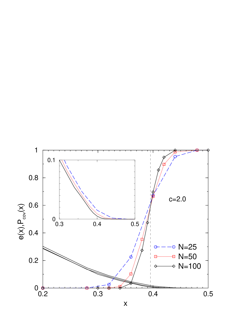
FIG. 1.: Probability $P_{cov}(x)$ that a cover exists for a random graph ($c=2$) as a function of the fraction $x$ of covered vertices. The result is shown for three different system sizes $N=25,50,100$ (averaged over $10^{4}$ - $10^{3}$ samples). Lines are guides to the eyes only. In the left part, where $P_{cov}=0$, the energy $e$ (see text) is positive. The inset enlarges this result the region $0.3\leq x\leq 0.5$.

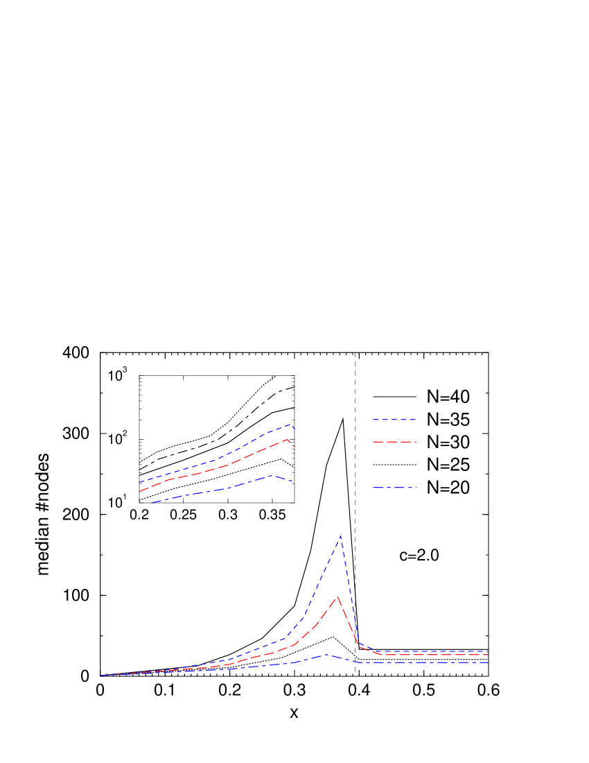
FIG. 2.: Time complexity of vertex cover: Median number of nodes visited in the backtracking tree as a function of the fraction $x$ of covered vertices for graph sizes $N=20,25,30,35,40$ ($c=2$). The inset shows the region below the threshold with logarithmic scale, including also data for $N=45,50$. The fact that in this representation the lines are equidistant shows that the time complexity grows exponentially with $N$.

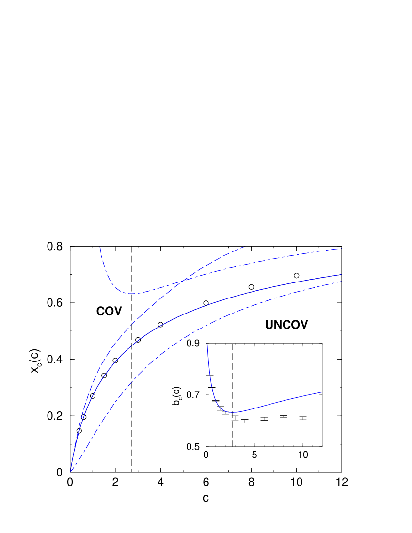
FIG. 3.: Phase diagram: critical fraction $x_{c}$ of covered vertices as a function of the edge density $c$. For $x>x_{c}(c)$, almost all graphs have VCs with $xN$ vertices, while they have almost surely no VC with $x<x_{c}(c)$. The solid line shows our analytic result. The rigorous bounds are given by dot-dashed [10] resp. dashed [11] lines. The vertical line is at $c=e$. The circles represent the results of the numerical simulations. Error bars are much smaller than symbol sizes. All numerical values were calculated from finite-size scaling fits of $x_{N,c}$ using functions $x_{N,c}=x_{c}(c)+aN^{-b}$. The inset shows the threshold backbone size $b_{c}$ as a function of $c$: analytical results are given by the solid line, numerical data by the error bars.

REFERENCES

- [1] M. R. Garey and D. S. Johnson, Computers and intractability (Freeman, San Francisco, 1979)
- [2] T. Hogg, B. A. Huberman, and C. Williams (eds.), Frontiers in problem solving: phase transitions and complexity, Artif. Intell. 81 (I+II) (1996)
- [3] D. Mitchell, B. Selman, and H. Levesque, in Proc. 10th Natl. Conf. Artif. Intell. (AAAI-92), 440 (AAAI Press/MIT Press, Cambridge, Massachusetts, 1992)
- [4] R. Monasson, R. Zecchina, Phys. Rev. E56, 1357 (1997)
- [5] R. Monasson, R. Zecchina, S. Kirkpatrick, B. Selman, and L. Troyansky, Nature 400, 133 (1999)
- [6] Informal: replica symmetry assumes that the VCs are collected in one cluster in configuration space, whereas replica-symmetry breaking corresponds to a large number of clusters.
- [7] G. Biroli, R. Monasson, and M. Weigt, Europ. Phys. J. B 14, 551 (2000)
- [8] P. Erdös and A. Rényi, Publ. Math. Inst. Hung. Acad. Sci. 5,17 (1960)
- [9] B. Bollobas, Random Graphs (Academic Press 1985)
- [10] P. G. Gazmuri, Networks 14, 367 (1984)
- [11] J. Harant, Discr. Math. 188, 239 (1998)
- [12] A. M. Frieze, Discr. Math. 81, 171 (1990)
- [13] E.L. Lawler and D.E. Wood, Oper. Res. 14, 699 (1966)
- [14] R.E. Tarjan and A.E. Trojanowski, SIAM J. Comp. 6, 537 (1977)
- [15] R. Monasson, J. Phys. A31, 513 (1998)
- [16] A. K. Hartmann, M. Weigt, in preparation.
- [17] is defined via .
- [18] Imagine there are two different values for resulting from different solutions of the saddle point equation. In between both, one would already imply a positive ground state energy, whereas the other would still be zero. Due to the standard procedure of taking saddle points with larger free energy in the replica approach, the positive energy solution has to be preferred, and hence the larger threshold.
- [19] I. Kanter and H. Sompolinsky, Phys. Rev. Lett. 58, 164 (1987)