Phase transitions in generalized chiral or Stiefel’s models

Abstract

We study the phase transition in generalized chiral or Stiefel’s models using Monte Carlo simulations. These models are characterized by a breakdown of symmetry $O(N)/O(N-P)$. We show that the phase transition is clearly first order for $N\geq 3$ when $P=N$ and $P=N-1$, contrary to predictions based on the Renormalization Group in $4-\epsilon$ expansion but in agreement with a recent non perturbative Renormalization Group approach.

P.A.C.S. numbers: 05.50.+q, 75.10.Hk,05.70.Fh, 64.60.Cn, 75.10.-b

I INTRODUCTION

The critical properties of frustrated spin systems are still under discussion [1]. In particular no consensus exists about the nature of the phase transition in canted magnetic systems. One example is the stacked triangular lattice with the nearest neighbor antiferromagnetic interactions (STA) with vector spins $O(N)$ where $N$ is the number of spin components which is always controversial [2, 3]. The non-collinear ground state due to the frustration leads to a breakdown of symmetry (BS) from $O(N)$ in the high temperature to $O(N-2)$ in the low temperature. This is different from ferromagnets in which the ground state is collinear and the BS is $O(N)/O(N-1)$. Based on the concept of universality, the class of the transition would be different in the two models. We generalize this chiral model for a BS of the type $O(N)/O(N-P)$. We obtain the STA model for $P=2$ while we obtain new BS for $N\geq P\geq 3$. For example, the case $N=P=3$ should correspond to real experimental systems, this is also applicable in spin glasses where some disorder is present. Several authors have already studied these generalized chiral models applying the Renormalization Group technic [4, 5, 6]. In mean field [5] for $N>P$ the model shows a usual second order type, but for $N=P$ the transition shows a special behavior. This last result could be interpreted with the BS in this case being $Z_{2}\otimes SO(N)$ and the coupling between the two symmetries leading to some special behavior (for example, the case $N=P=2$ in two dimensions (d) is always very debated [7]). The $d=4-\epsilon$ expansion gives more information. The picture is very similar for all $N\geq P\geq 2$ (for details see [3] and references therein). At the lowest order in $\epsilon$, there are up to four fixed points, depending on the values of $N$ and $P$. Amongst them are the trivial Gaussian fixed point and the standard isotropic $O(NP)$ Heisenberg fixed point. These two fixed points are unstable. In addition, a pair of new fixed points, one stable and the other unstable, appear if the case is $N\geq N_{c}(d)$ with [6]

$$N_{c}(d)=5P+2+2\sqrt{6(P+2)(P-1)}-\bigg{[}5P+2+{25P^{2}+22P-32\over 2\sqrt{6(P+2)(P-1)}}\bigg{]}\,\epsilon\,.$$ (1)

For $P=2$ we find the standard result $N_{c}=21.8-23.4\,\epsilon$. On the other hand, for $P=3$ we obtain $N_{c}=32.5-33.7\,\epsilon$ and for $P=4$ we obtain $N_{c}=42.8-43.9\,\epsilon$. A ”tricritical” line exists which divides a second order region for low $d$ and large $N$ from a first order region for large $d$ and small $N$. From these results Kawamura, using $\epsilon=1$ ($d=3$), obtained that $N_{c}(d=3)<0$ for all $P$. Thus he concluded that the experimental or numerical accessible systems ($N>0$) were in the second order region. Unfortunately it has been proved that the results of $4-\epsilon$ are, at best, asymptotic [8]. They have to be resummed to obtain reliable results. Indeed for $P=2$ the calculation of the next order in $\epsilon$, combined with a resummation technic, leads the experimental accessible systems for $N=2$ or $N=3$ in the first order region [9, 10]. We believe that the same applies for $P\geq 3$. In order to verify our assumption, we have done some simulations for $P=3$ and $P=4$ with $N=P$ and $N=P+1$. The most interesting case is $P=N=3$ with some possible experimental realizations and connection with the spin glasses. Moreover it is meaningful to study the generalized model in order to have a better overview. The system we analyze is the Stiefel model [11]. This model is constructed to have the needed BS. It is closely connected to real systems with complicating interactions, which are characterized by the same BS (for the case $P=2$ see [3] and reference therein). From the principle of universality, models with the same BS should belong to the same universality class. Moreover we have shown that the use of the Stiefel model allows us to avoid problems which are seen in standard models, such as the presence of a complex fixed point (or minimum in the flow) [2, 3].

In the following section II the studied models are presented, we describe the details of the simulations and the finite size scaling analysis. Results will be given in section III and the last section is devoted to the conclusion.

II Stiefel’s models, Monte Carlo simulations and first order transitions

In this section we introduce different models studied in this work.

First the $V_{3,3}$ model which is represented in Fig. 8. The energy of the model is

$$H=J\sum_{ij}\sum_{k=1}^{P}\Big{[}\ {\bf e}_{k}(i)\cdot{\bf e}_{k}(j)\ \Big{]}$$ (2)

where the $P$ mutual orthogonal $N$ component unit vectors ${\bf e}_{k}(i)$ at lattice site $i$ interact with the next $P$ vectors at the neighboring sites $j$. The interaction constant is here negative to favor alignment of the vectors at different sites. Taking a strict orthogonality between the vectors is similar to removing ”irrelevant” modes corresponding to the variation between the spins inside the cell. For example, in the case of a triangular lattice with antiferromagnetic interactions (STA) we force the three spins of each cell to have a rigidity constraint with the sum of all the spins being always zero. The obtained model is equivalent to the STA at the critical temperature and can easily be transformed into the Stiefel’s $V_{3,2}$ model (for more detail see [2, 3]).

We did not use the clusters algorithm [3] because it gives worse results than the standard Metropolis algorithm for first order transitions.

The method for choosing the random vector depends on the number of components $N$. For $N=3$ we follow the method explained in [3] for the direct-trihedral model. We construct two orthogonal vectors ${\bf e_{1}}$ and ${\bf e_{2}}$, and the third vector is constructed by the vector product of the first two:

$${\bf e_{3}}=\sigma\ {\bf e_{1}}\times{\bf e_{2}}\$$ (3)

where $\sigma$ is a random Ising variable, corresponding to the Ising symmetry present in the $V_{3,3}$ model. This is the difference with the direct-trihedral model defined in [3], where no Ising symmetry is present.

To simulate the $V_{4,3}$ model we follow a similar procedure. We construct now three orthogonal unit vectors, ${\bf e}_{k}=(e_{k}^{1},e_{k}^{2},e_{k}^{3},e_{k}^{4})$ with $k=1,\,2,\,3$, randomly in four dimensions using six Euler angles. The first $\theta_{0}$ must be chosen with probability $\sin(\theta_{0})^{2}\,d\theta_{0}$, two other with probability $\sin(\theta_{1,2})\,d\theta_{1,2}$ and the rest three $\theta_{3,4,5}$ with probability $\theta_{3,4,5}$. We obtain for ${\bf e_{1}}$:

$$e_{1}^{1}= -\cos(\theta_{3})*\cos(\theta_{1})*\sin(\theta_{5})*\cos(\theta_{2})*\cos(\theta_{4})$$ (4)

$$-\cos(\theta_{3})*\cos(\theta_{1})*\cos(\theta_{5})*\sin(\theta_{4})$$ (5)

$$+\cos(\theta_{3})*\sin(\theta_{1})*\sin(\theta_{5})*\sin(\theta_{2})*\cos(\theta_{0})$$ (6)

$$+\sin(\theta_{3})*\sin(\theta_{5})*\cos(\theta_{2})*\sin(\theta_{4})$$ (7)

$$-\sin(\theta_{3})*\cos(\theta_{5})*\cos(\theta_{4})$$ (8)

$$e_{1}^{2}= -\sin(\theta_{3})*\cos(\theta_{1})*\sin(\theta_{5})*\cos(\theta_{2})*\cos(\theta_{4})$$ (9)

$$-\sin(\theta_{3})*\cos(\theta_{1})*\cos(\theta_{5})*\sin(\theta_{4})$$ (10)

$$+\sin(\theta_{3})*\sin(\theta_{1})*\sin(\theta_{5})*\sin(\theta_{2})*\cos(\theta_{0})$$ (11)

$$-\cos(\theta_{3})*\sin(\theta_{5})*\cos(\theta_{2})*\sin(\theta_{4})$$ (12)

$$+\cos(\theta_{3})*\cos(\theta_{5})*\cos(\theta_{4})$$ (13)

$$e_{1}^{3}= -\sin(\theta_{5})*\sin(\theta_{2})*\sin(\theta_{0})$$ (14)

$$e_{1}^{4}= \sin(\theta_{1})*\sin(\theta_{5})*\cos(\theta_{2})*\cos(\theta_{4})$$ (15)

$$+\sin(\theta_{1})*\cos(\theta_{5})*\sin(\theta_{4})$$ (16)

$$+\cos(\theta_{1})*\sin(\theta_{5})*\sin(\theta_{2})*\cos(\theta_{0})$$ (17)

for ${\bf e_{2}}$:

$$e_{2}^{1}= \sin(\theta_{0})*\sin(\theta_{1})*\cos(\theta_{3})$$ (18)

$$e_{2}^{2}= \sin(\theta_{0})*\sin(\theta_{1})*\sin(\theta_{3})$$ (19)

$$e_{2}^{3}= \cos(\theta_{0})$$ (20)

$$e_{2}^{4}= \sin(\theta_{0})*\cos(\theta_{1})$$ (21)

and for ${\bf e_{3}}$:

$$e_{3}^{1}= \cos(\theta_{3})*\sin(\theta_{2})*\cos(\theta_{4})*\cos(\theta_{1})$$ (22)

$$+\cos(\theta_{3})*\cos(\theta_{2})*\cos(\theta_{0})*\sin(\theta_{1})$$ (23)

$$-\sin(\theta_{2})*\sin(\theta_{4})*\sin(\theta_{3})$$ (24)

$$e_{3}^{2}= \sin(\theta_{3})*\sin(\theta_{2})*\cos(\theta_{4})*\cos(\theta_{1})$$ (25)

$$+\sin(\theta_{3})*\cos(\theta_{2})*\cos(\theta_{0})*\sin(\theta_{1})$$ (26)

$$+\sin(\theta_{2})*\sin(\theta_{4})*\cos(\theta_{3})$$ (27)

$$e_{3}^{3}= -\cos(\theta_{2})*\sin(\theta_{0})$$ (28)

$$e_{3}^{4}= -\sin(\theta_{2})*\cos(\theta_{4})*\sin(\theta_{1})$$ (29)

$$+\cos(\theta_{2})*\cos(\theta_{0})*\cos(\theta_{1})\ .$$ (30)

From this model we can easily create the direct-quadrihedral model and the $V_{4,4}$, these two models being composed of four orthogonal vectors with four components. The differences between the two models are the presence of an Ising variables in the $V_{4,4}$ where right handed and left handed are allowed while only one possibility exists in the direct-quadrihedral. The direct-quadrihedral and the $V_{4,3}$ models are topologically equivalent, they should have the same low energy physics and therefore belong to the same universality class. The connection between the direct-trihedral and the $V_{3,2}$ models [3] is very similar to the above. We form a fourth vector from the vector product of ${\bf e_{1}}$, ${\bf e_{2}}$ and ${\bf e_{3}}$:

$${\bf e_{4}}={\bf e_{1}}\times{\bf e_{2}}\times{\bf e_{3}}\$$ (31)

for the direct-quadrihedral model, and we add a random Ising variable $\sigma$ to the $V_{4,4}$ model:

$${\bf e_{4}}=\sigma\ {\bf e_{1}}\times{\bf e_{2}}\times{\bf e_{3}}\ .$$ (32)

We follow the standard Metropolis algorithm to update one $P$-hedral after the other. In each simulation between 20 000 to 100  000 Monte Carlo steps are made for equilibration and averages. Cubic systems of linear dimensions from $L=10$ to $L=25$ are simulated.

The order parameter $M$ for this model is

$$M={1\over P\,L^{3}}\,\sum_{i=1}^{P}\,\big{|}\,M_{i}\big{|}$$ (33)

where $M_{i}$ is the total magnetization given by the sum of the vectors ${\bf e}_{i}$ over all sites and $L^{3}$ is the total number of sites.

For $N=P$ we define a chirality order parameter:

$$\kappa={1\over L^{3}}\,{\bf e_{P}}.(\,\prod_{i=1}^{P-1}\,{\bf e_{i}}\,)$$ (34)

where ${\prod}$ means the vector product $\times$.

We use the histogram MC technique developed by Ferrenberg and Swendsen [12] which is very useful for identifying a first order transition.

The finite size scaling (FSS) for a first order transition has been extensively studied [13, 14, 15]. A first order transition can be identified by some properties and in particular by the following:

• The histogram $P(E)$ has a double peak.

• The magnetization, the chirality and the energy have hysteresis.

The double peak in P(E) means that at least two states with different energies coexist in the system at one temperature.

III Results

We now present our results for the different models. The $V_{3,3}$ and the $V_{4,4}$ show a strong first order transition. The hysteresis in $E$ and $<M>$ are shown in Fig. 8 and 8 for the $V_{3,3}$ model, and in $E$ and $\kappa$ for the $V_{4,4}$ model in Fig. 8 and 8. This is in accordance with the negative $\eta$ exponent for the $V_{3,3}$ model found in [11] which describes a first order transition because $\eta$ must be positive [3, 16, 17]. This result is understandable because there is a coupling between the Ising symmetry and the $SO(N)$ symmetry. We notice that the $V_{2,2}$ model is also of first order [2] and that the models have a stronger first order transition if $N$ is greater (we obtain the same hysteresis for $L=20$ for the $V_{3,3}$ as for $L=10$ for the $V_{4,4}$). Thus we can generalize our result that the transition is always of first order for $N=P$.

The $V_{4,3}$ model shows no hysteresis. However a double peak structure appears in the energy histogram and becomes more apparent when the size increases (Fig. 8). For greater sizes the two peaks are well separated by a region of zero probability, the transition time from one state to the other grows exponentially with the size of the lattice. We should obtains hysteresis in the thermodynamic quantities when the simulation is not too long. The $V_{4,3}$ model has a first order transition but weaker than the direct-quadrihedral model which, for similar sizes, shows hysteresis. As explained above the two models belong to the same universality class, i.e. a first order transition, similar to the dihedral model $V_{3,2}$ and the direct-trihedral model [3]. The addition of the fourth leg to the $V_{4,3}$ model allows the first order behavior to be more clearly visible. In Fig. 8 we have plotted our hypothesis for the RG diagram flow. Following the initial point, the flow could be under the influence of a ”complex” fixed point (or minimum of the flow [5]) and the system mimics a second order transition. Well outside the influence of this fixed point the transition is strongly of first order and in the crossover between these two regions the transition is weakly first order. For a more developed discussion see [3].

IV Conclusion

We have tried to give a general picture of the transition with a $O(N)/O(N-P)$ breakdown of symmetry. We have shown by numerical simulations that for $N=P=3$ and $N=P=4$, the transition is clearly of first order. We have generalized our result for all $N=P$. A similar conclusion is obtained for $N=4$ and $P=3$. Using the fact that for $N=3$ and $P=2$ the transition is also of first order, we can generalize our result for all $P=N-1$. This is in contradiction with to the conclusion of Kawamura [6] which is based on two loops of a $4-\epsilon$ expansion. As we have noted the $\epsilon$ expansion has to be resummed to obtain reliable results. We can try to achieve this by forming simple Padé approximants. For a function $f=a+b\,\epsilon$ we obtain the approximation $f=1/(1-\epsilon\,b/a)$ which we apply to $\epsilon=1$ ($d=3$) and $P=$2, 3 and 4. We obtain $N_{c}(P=2)\sim 10$, $N_{c}(P=3)\sim 16$ and $N_{c}(P=2)\sim 21$. Unfortunately the results can not be perfect and in particular the result for $P=2$ is not close enough to the result including the next order expansion $N_{c}=3.39$ [10] which demonstrates that the lower-order $\epsilon$ expansions are useless in this case. However we remark that the $N_{c}$ ”resummed” increases with $P$ which is in agreement with our result, i.e. that the initial point in the renormalization flow is farther away from the mimic of the second order region [3]. Thus the systems will show a stronger first order transition. This result matches with a recent study on the case $P=N=3$ which is based on a non perturbative Renormalization Group procedure [18]. We conclude that transitions for $N=P$ and $N=P+1$ are of first order for all $N$.

V Acknowledgments

This work is supported by the Alexander von Humboldt Foundation. The authors are grateful to Professors B. Delamotte, G. Zumbach, and K.D. Schotte for discussions.

FIG. 1.: Stiefel’s model $V_{3,3}$ and their interactions. ${\bf e}_{1}(i)$ interacts only with ${\bf e}_{1}(j)$, neither with ${\bf e}_{2}(j)$ which interacts with ${\bf e}_{2}(i)$, nor with ${\bf e}_{3}(j)$ which interacts with ${\bf e}_{3}(i)$.

FIG. 2.: Internal energy per spin $E$ versus T for the $V_{3,3}$ model. Lines are guides to the eye. The arrows indicate if the MC simulation is cooling (circle) or heating (square) the system. The system size is $L=20$. A hysteresis is clearly visible.

FIG. 3.: Magnetization versus T for the $V_{3,3}$ model. The size of the system is $L=20$. See comments in Fig. 8

FIG. 4.: Internal energy per spin $E$ versus T for the $V_{4,4}$ model. The system size is $L=10$. See comments in Fig. 8

FIG. 5.: Chirality versus T for the $V_{4,4}$ model. The system size is $L=10$. See comments in Fig. 8

FIG. 6.: Energy histogram $P(E)$ as a function of the energy per site $E$ for the $V_{4,3}$ model for various sizes $L$ at different temperatures of simulation $T_{L}$: $T_{15}=1.1802$, $T_{20}=1.1771$, $T_{25}=1.1758$.

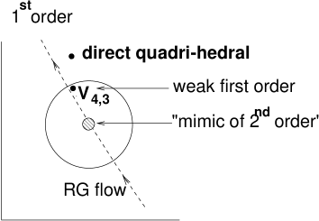
FIG. 7.: Internal energy per spin $E$ versus T for the direct-quadrihedral model. The system size is $L=20$. See comments in Fig. 8

FIG. 8.: Hypotheses of Hamiltonian flows induced by renormalization-group transformations. The arrows (dashed line) indicate the direction of flow under iteration.

REFERENCES

- [1] Magnetic Systems with Competing Interactions (Frustrated Spin Systems), edited by H.T. Diep (World Scientific, Singapore, 1994).
- [2] D. Loison and K.D. Schotte, Eur. Phys. J. B 5, 735 (1998)
- [3] D. Loison and K.D. Schotte, to be published in Eur. Phys. J. B, accessible at http://www.physik.fu-berlin.de/∼loison/articles/reference10.html
- [4] L. Saul, Phys. Rev. B 46, 13847 (1992)
- [5] G. Zumbach Nucl. Phys. B 413,771 (1994).
- [6] H. Kawamura, J. Phys. Soc. Jpn 59, 2305 (1990)
- [7] E. Granato and M.P. Nightingale Physica B 222, 266 (1996), P. Olson Phys. Rev. B 55 3585 (1997).
- [8] J.C. Le Guillou and J. Zinn-Justin, J. Phys. (Paris) Lett. 46, L137 (1985)
- [9] S.A. Antonenko and A.I. Sokolov, Phys. Rev. B 49, 15901 (1994).
- [10] S.A. Antonenko, A.I. Sokolov and V.B. Varnashev, Phys. Lett. A 208, 161 (1995).
- [11] H. Kunz and G. Zumbach,J. Phys. A 26, 3121 (1993).
- [12] A. M. Ferrenberg and R. H. Swendsen, Phys. Rev. Let. 61, 2635 (1988), Phys. Rev. Let. 63, 1195 (1989).
- [13] V. Privman and M.E. Fisher, J. Stat. Phys. 33, 385 (1983).
- [14] K. Binder, Rep. Prog. Phys. 50, 783 (1987)
- [15] A. Billoire, R Lacaze and A. Morel, Nucl. Phys. B 370 773 (1992).
- [16] A.Z. Patashinskii and V.I. Pokrovskii, Fluctuation Theory of Phase Transitions, (Pergamon press 1979), §VII, 6 , The S-matrix method and unitary relations.
- [17] J. Zinn-Justin, Quantum Field Theory and Critical Phenomena, (Oxford University Press, Oxford, 1996), §7.4 Real-time quantum field theory and S-matrix, §11.8 Dimensional regularization, minimal subtraction: calculation of RG functions.
- [18] M. Tissier, D. Mouhanna, B. Delamotte, cond-mat/9908352