First and second order transition of frustrated Heisenberg spin systems

Abstract

Starting from the hypothesis of a second order transition we have studied modifications of the original Heisenberg antiferromagnet on a stacked triangular lattice (STA–model) by the Monte Carlo technique. The change is a local constraint restricting the spins at the corners of selected triangles to add up to zero without stopping them from moving freely (STAR–model). We have studied also the closely related dihedral and trihedral models which can be classified as Stiefel models. We have found indications of a first order transition for all three modified models instead of a universal critical behavior. This is in accordance with the renormalization group investigations but disagrees with the Monte Carlo simulations of the original STA–model favoring a new universality class. For the corresponding $x$–$y$ antiferromagnet studied before, the second order nature of the transition could also not be confirmed.

P.A.C.S. numbers:05.70.Fh, 64.60.Cn, 75.10.-b

1 INTRODUCTION

The critical properties of frustrated spin systems are still under discussion [1]. In particular no consensus exists about the nature of the phase transition of an antiferromagnet on a stacked triangular lattice with nearest neighbor interactions. The symmetry group for a Heisenberg antiferromagnet at high temperatures $SO_{3}$ changes to $SO_{2}$ for the usual antiferromagnet, but the symmetry is completely broken in the low temperature phase of the frustrated antiferromagnet. This difference in the breakdown of symmetry between the frustrated and non frustrated cases should lead to different classes of critical behavior. The controversial point for the stacked triangular antiferromagnet (STA) is whether the phase transition is of second order with a new chiral universality class [2] or whether its true nature is a weak first order change.

Monte Carlo studies [3, 4, 5, 6, 7, 8] favor a new universality class whereas renormalization group studies indicate a first order transition, since no stable fixed point can be found for the Heisenberg case in order $\epsilon^{2}$ with $\epsilon=4-d$ (d is the dimension of space) [9] and also for an expansion up to three loops in $d=3$ [10]. The results for the critical exponents of the numerous Monte Carlo simulations are listed in table 1. They agree reasonably well and also with the experimental values in table 2. One notices that the new critical indices are quite distinct from the standard ones for the Heisenberg model with symmetry breaking $SO_{3}/SO_{2}$ listed in table 3. The only flaw is the small negative values of $\eta$, since this exponent should always be positive [11, 12].

The discrepancy between the renormalization group analysis and the Monte Carlo simulation can be removed by assuming that the first order phase transition occurs with a correlation length larger than the diameter of the cluster studied. Since this size cannot be substantially increased with the present technical means and skills we have tried to investigate modified lattice spin systems which should belong to the same universality class. The idea is to shorten the correlation length by these modifications in order to reveal the first order nature of the transition. This strategy was successful for the $x$–$y$ STA–model we investigated before [13] and we could show that in fact the phase transition is of first order in this case.

Following Zumbach [14] one can analyze such a weak first order transition in terms of the renormalization group approach as due to a fixed point in the complex parameter space (More precisely it is only necessary to have a minimum in the RG flow). A basin of attraction for the real parameters will be generated and “mimic” a second order transition with slightly changed scaling relations. The unphysical negative values of $\eta$ in table 1 could be corrected using Zumbach’s approach.

Investigations about the phase transitions of the STA–systems and similar helimagnetic systems [7, 8] are not only of interest for the field of magnetism including the experimental studies. Phase transitions in superfluids, in type II superconductors, and in smectic–A liquid crystals should be similar in nature to the ones of frustrated Heisenberg magnets.

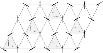
Figure 3: Ground state configuration for the STA and the STAR model. The supertriangles are shaded. The dihedral are drawn at the center of each supertriangle.

Figure 4: The interaction between the “spins” or dihedrals $i$ and $j$ of Stiefel’s model $V_{3,2}:$ where ${\bf e}_{1}(i)$ interacts only with ${\bf e}_{1}(j)$ and ${\bf e}_{2}(i)$ with ${\bf e}_{2}(j)$.

The numerical simulations are closely connected to a similar study for the $x$–$y$ spins [13]. We study the classical Heisenberg spin system on the stacked triangular lattice by fixing for selected triangles the spin direction to a 120^∘–order which would correspond to the ideal antiferromagnetic order on a triangular lattice as in Fig. 4. The common orientation of a 120^∘–cluster is still free. The principle behind this construction is that modes removed by the 120^∘–rigidity are “irrelevant” close to the critical temperature. What is relevant is the common direction and orientation. The antiferromagnet STA and the rigid antiferromagnet STAR should therefore be in the same universality class. These considerations can also be applied to Stiefel’s $V_{3,2}$ or dihedral model [15]. A third model studied is the right handed trihedral model. It is constructed by adding a third vector given by the vector product of the two of the dihedron. As we do not add new degrees of freedom the model should again belong to the same universality class.

That the behavior close to the phase transition should not change if one modifies the models by constraints can only be expected from a second order transition. However, if one assumes that the transition is of first order, but not visible since the barriers between the two phases are too low for the spin clusters one can simulate, then building in constraints in the models and simulations should make a difference since the barriers are more difficult to overcome.

In section II we present a review of the RG studies. In the following section the three models studied are presented. The details of the simulations and the finite size scaling analysis are described in section IV. Results are given in section V. The discussion is in section VI where we will review also the experimental studies and the other RG studies in $2+\epsilon$ expansions.

2 Renormalization group studies and complex fixed points

2.1 Renormalization group studies in $d=3$ and $d=4-\epsilon$

The renormalization group studies have motivated for the re-analysis of the frustrated Heisenberg antiferromagnet with the Monte Carlo technique. Therefore we repeat briefly the main points. For more details we refer to Antonenko and Sokolov [10].

The Hamiltonian one considers is

$$H={1\over 2}\int d^{3}x\Bigl{[}r_{0}^{2}\,\phi_{\alpha}\phi_{\alpha}^{*}+\nabla\phi_{\alpha}\nabla\phi_{\alpha}^{*}+{u_{0}\over 2}\phi_{\alpha}\phi_{\alpha}^{*}\phi_{\beta}\phi_{\beta}^{*}+{w_{0}\over 2}\phi_{\alpha}\phi_{\alpha}\phi_{\beta}^{*}\phi_{\beta}^{*}\,\Bigr{]}$$ (1)

with $\phi_{\alpha}$ a complex vector order parameter field. Summation of repeated indices $\alpha,\,\beta=1,\,\dots N$ is implied with $N=3$ for the Heisenberg case. The deviation from the transition temperature is given by $r_{0}^{2}$ and there are two coupling constants $u_{0}$ and $w_{0}$, both positive for a non–collinear ground state, that is the two vectors forming the complex vector $\phi$ should not be parallel. For the non frustrated case there is only one field and one coupling constant, but for the superfluid ³He the above complexity also arises [16, 17].

Renormalization group calculations for $d=4-\epsilon$ [16, 18, 2] or also directly for $d=3$ [10] show that four fixed points exist:

• The Gaussian fixed G point at $u^{*}=v^{*}=0$ with mean field critical exponents.

• The $O(2N)$ fixed point H at $w^{*}=0$ and $u^{*}=u_{H}\neq 0$ with $O(2N)$ exponents (see table 3).

• Two fixed points $F_{+}$ and $F_{-}$ at location ($u_{F_{+}},w_{F_{+}})$ and $(u_{F_{-}},w_{F_{-}}$) different from zero. These are the fixed points associated with a new ”chiral” universality class.

The existence and stability of the fixed points depend on the number of components $N$:

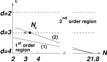
Figure 1: a), b), c) Hamiltonian flow induced by renormalization group transformations. The arrows indicate the direction of flow under iterations. d) For $N<N_{c}$ the fixed points $F_{+}$ and $F_{-}$ become complex.

Figure 2: The critical curve $N_{c}(d)$ separating the first order region at small $N$ and large $d$ from the second order region for large $N$ and low $d$. Curve (1) is the result of first order in $\epsilon=d-4$, and curve (2) in second order. The STA at $d=N=3$ is marked by a cross. In contrast to curve (1) curve (2) lets the physical relevant systems $N=2,\,3$ stay inside the first order region.

• $N>N_{c}$: four fixed points are present but three are unstable ($G$, $H$, $F_{-}$) and the stable one is $F_{+}$. Therefore the transition belongs to a new universality class different from the standard $O(N)$ class. If the initial point for the RG flow is to the left of the line ($G,\,F_{-}$), see fig. 2 a. the flow is unstable and the transition will be of first order.

• $N=N_{c}$: the fixed points $F_{-}$ and $F_{+}$ coalesce to a marginally stable fixed point. One would think that the transition is “tricritical” but the exponents are different and not given by the tricritical mean field values. The reason is that there are two quartic coupling constants not zero, see Fig. 2 b, in contrast to the tricritical $O(N)$ point where the quartic term disappears and a sextic term takes over [19].

• $N<N_{c}$: F_- and $F_{+}$ move into the complex parameter space, see fig. 2 c and d. The absence of stable fixed points is interpreted as a signature of a first order transition.

The difficulty is to find a reliable value for $N_{c}$. The dependence on $d$ has been calculated to first order in $\epsilon=4-d$ [16, 18] as

$$N_{c}=\,21.8-23.4\,\epsilon\ .$$ (2)

In repeating the analysis for the triangular antiferromagnet and choosing $\epsilon=1$ for $d=3$ Kawamura [2] has argued that the $XY$ and Heisenberg cases should be above $N_{c}$, motivated by Monte Carlo calculations which supported a second order transition of a new universality class [3, 4, 5, 6, 7, 8] with critical exponents for the Heisenberg case $\nu=0.59$, $\beta=0.29$ (see table 1) different from the standard ones.

Of course the results linear or higher in $\epsilon$ are at best asymptotic [20]. Antonenko, Sokolov and Varnashev extended the analysis to $\epsilon^{2}$ [9]. For an analysis directly in three dimensions see [10]. For the critical number of components after resummation

$$N_{c}=3.91(1)\$$ (3)

is obtained by the direct method [10] and $N_{c}=3.39$ with the $\epsilon$ expansion to second order [9]. In Fig. 2 the results of the RG studies are depicted. There is a line which separates a region of first order transition for high dimensions and low $N$ (Fig. 2c) from a region of second order transition for low dimensions and high $N$ (Fig. 2a). The transition on this line is special (Fig. 2b) but is not the standard tricritical.

Similar considerations have been applied to the normal to superconducting type II transition. Starting point is the Ginzburg–Landau Hamiltonian with also two coupling constants, a quartic coupling and the coupling to the magnetic field. Expanding to first order in $\epsilon=4-d$ Halperin et al. [21] and Chen et al. [22] arrived at results almost identical to the ones for frustrated magnets. There are also four fixed points with one stable one if the number of order parameters $N$ exceeds $N_{c}=365.9$ for a fictitious superconductor in 4 dimensions. The unstable $0(2N)$ fixed point is replaced by an $XY$ fixed point. For $N<N_{c}$ only the unstable Gaussian and this unstable $XY$ fixed point are present, and the question whether the physical relevant $N=2$ case is of second order or not can also not be answered, although the value of $N_{c}$ in two loop order has been calculated [23]: $N_{c}=365.90-640.76\,\epsilon+O(\epsilon^{2})\$. If we put $\epsilon=1$ we obtain $N_{c}(d=3)\approx-275$ which is less than two and the transition should be of second order. The nematic-to-smectic-A transition in liquid crystals is described by a model similar to the Ginzburg–Landau Hamiltonian transition [24, 25] and again the problem of second or first order transition arises [21, 26].

The superfluid phase transitions of He³ and the phase transitions of helimagnets were first studied with the field theoretical approach (1) by Love, More, Jones and Bailin [16, 17] and by Garel and Pfeuty [18] respectively. In principle all the considerations should also be applicable to these systems, however for He³ the critical region is not really accessible. Returning to the frustrated antiferromagnets and accepting the value $N_{c}=3.91$ for $d=3$ of eq. 3, the $XY$ and Heisenberg systems and also the helimagnets should have a first order transition in three dimensions.

2.2 Almost second order transitions and complex fixed points

The discrepancy between the results of RG studies which indicate a first order transition and the results of Monte Carlo study which favor a second order transition (see table 1) can be removed by using complex fixed points in the RG analysis. Indeed, as $N_{c}$ is very close to $N=3$ the fixed points $F_{+}$ and $F_{-}$ will not be far off from the real space of parameters $u^{*}$ and $v^{*}$ at $N_{c}$ as depicted in fig. 2 d. Zumbach [14] has studied in detail the influence of a complex fixed point on the RG analysis. The basin of attraction of such a complex fixed point will mimic a second order transition with modified scaling relations

$$2\,\beta = \nu\,(d-2+\eta-c_{\beta})$$ (4)

$$\gamma = \nu\,(2-\eta+c_{\gamma})\ .$$ (5)

The constants $c_{\beta}$ and $c_{\gamma}$ are corrections of the scaling relations absent if the fixed point is real. Using these relations to determine $\eta$ without corrections we get a negative value for $\eta$. Since $\eta$ must be positive [11] or at least zero we have an estimate for $c_{\beta,\gamma}$ and an indication that the transition is not a real second order one. We have used this criterion before for $x$–$y$ case [13]. The essential point is the smallness of $\eta$, approximately $\eta\approx 0.03$ for magnets, so that the correction terms $c_{\beta,\gamma}$ are clearly visible.

A negative $\eta$ is unphysical since unitarity would be violated in the corresponding quantum field theory [11, 12, 27]. For spin glasses this restriction no longer holds and indeed a negative $\eta$ can be obtained [28]. Also for superconductors a negative $\eta$ have been found [22] influenced by the choice of gauge [29]. The critical exponents must be gauge-independent and in a recent study [30] it has been shown that $\eta$ is positive for superconductors.

Using the local potential approximation for the RG the critical exponent $\nu$ can be calculated for real and complex fixed points (more precisely for a minimum in the flow) following Zumbach [14]. In this approximation $\eta$ is zero and the result will have errors of a few percents, for example 8% for the Heisenberg ferromagnet [31]. For the fixed point $F_{+}$ of the frustrated systems Zumbach obtains $\nu\simeq 0.63$ for $N=3$. This result is compatible with $\nu=0.59(1)$ obtained by MC calculations for Heisenberg spins on a stacked triangular lattice (see table 1).

By the same approximation Zumbach estimated the interval where the systems should be under the influence of a complex fixed point as

$$2.58<N<4.7\ \>.$$ (6)

Outside of these limits for $N<2.58$ the transition is of first order and for $N>4.7$ the transition belongs to the new universality class. The two values $N_{c}=4.7$ for the local potential approximation and $N_{c}=3.91(1)$ found by Antonenko and Sokolov [10] by field theoretical means are not so different. The minimum limit 2.58 is in agreement with our simulations for the Stiefel model. The transition is indeed of first order for $N=2$ [13] and it will be shown here that the $N=3$ case has a pseudo second order behavior.

3 Models and simulations

In this section we introduce briefly different models that we use in this work. A more complete presentation can be found in [13].

3.1 The STAR model

For the stacked triangular antiferromagnet (STA) we take the simplest Hamiltonian with one exchange interaction constant $J>0$ (antiferromagnetic).

$$H=\sum_{(ij)}J_{ij}\,{\bf S}_{i}.{\bf S}_{j}\ ,$$ (7)

where ${\bf S}_{i}$ is a three component spin vector of unit length, and the sum is over all neighbor spin pairs of the lattice. There are six nearest neighbor spins in the plane and two in adjacent planes. In the ground state the spins are in a planar arrangement with the three spins at the corners of each triangle forming a 120^∘ structure (see Fig. 4).

For one triangle the spin vectors obey the equation

$${\bf S}_{1}+{\bf S}_{2}+{\bf S}_{3}={\bf 0}\ .$$ (8)

where the indices refer to the three corners. To get the STAR model one imposes this equation as a restriction for the spin directions valid at all temperatures. In this theory the local fluctuations violating this constraint become modes with a gap. Thus they do not contribute to the critical behavior and can be neglected. However, one can do this only for selected triangles, for instance the shaded ones in fig. 4, otherwise the spin configuration would be completely frozen.

The lattice is partitioned into interacting triangles which do not have common corners, so that each spin belongs only to one triangle. For the Monte Carlo simulation one spin direction (two degrees of freedom) is chosen and then the direction of the second spin selected in the cone of 120^∘ around the first one. The third is determined by the constraint (8). All the spins of the supertriangles (the shaded ones) have, only in the ground state, the same orientation. At finite temperatures there is a perfect order within a supertriangle, but fluctuations of the orientation between these triangles occur.

The Monte Carlo updating for the state of the supertriangle is done the following way. First two orthogonal unit vectors are chosen at random in three dimensions. One needs three Euler angles to do this, the first $\theta_{0}$ must be chosen with probability $\sin(\theta_{0})\,d\theta_{0}$ and the other two $\theta_{1,2}$ with probability $\theta_{1,2}$ so that

$${\bf u} = \pmatrix{\sin(\theta_{0})\cos(\theta_{1})\cr\sin(\theta_{0})\sin(\theta_{1})\cr\cos(\theta_{0})\cr}$$ (9)

$${\bf v} = \pmatrix{-\sin(\theta_{1})\cos(\theta_{2})-\cos(\theta_{0})\cos(\theta_{1})\sin(\theta_{2})\cr\cos(\theta_{1})\cos(\theta_{2})-\cos(\theta_{0})\sin(\theta_{1})\sin(\theta_{2})\cr\sin(\theta_{0})\sin(\theta_{2})\cr}$$ (10)

Then the three spin vectors on each supertriangle are determined by

$${\bf S_{1}} = {\bf u}$$

$${\bf S_{2}} = \cos(120^{\circ})\,{\bf u}+\sin(120^{\circ})\,{\bf v}$$ (11)

$${\bf S_{3}} = \cos(240^{\circ})\,{\bf u}+\sin(240^{\circ})\,{\bf v}\ .$$

The interaction energy between the spins of this supertriangle with the spins of the neighboring ones is calculated in the usual way. We follow the standard Metropolis algorithm to update one supertriangle after the other. One million MC–steps for equilibration are carried out and up to six million steps were used for the largest sizes to obtain reliable averages. Long enough simulations are necessary because the critical slowing down is strong.

The number of spins is given by $N=L\times L\times L_{z}$, where $L\times L$ gives the number of spins in one plane and $L_{z}=2\,L/3$ the number of planes. Simulations have been done for $L=18,\,21,\,24,\,30,\,36,\,42$, where L must be a multiple of 3 in order to use periodic boundary conditions and to avoid frustration effects in the planes.

The order parameter $M$ used in the calculations is

$$M={1\over N}\,\sum_{i=1}^{3}|\,M_{i}|\$$ (12)

where the magnetization $M_{i}$ is defined on one of the three sublattices. This definition generalizes the one used for two collinear sublattices.

3.2 The Stiefel model

The Stiefel model $V_{3,2}$, that is a “Zweibein” (or dihedral model) in three dimensional space is a further abstraction of the constrained three spin system discussed in the previous section. The three spins at the corner of a triangle can be taken as a planar or degenerate “Dreibein” where the third leg is a linear combination of the other two and can be left out. The energy is given by

$$H=J\sum_{ij}\Big{[}\ {\bf e}_{1}(i)\cdot{\bf e}_{1}(j)\,+\,{\bf e}_{2}(i)\cdot{\bf e}_{2}(j)\ \Big{]}$$ (13)

where the mutual orthogonal three component unit vectors ${\bf e}_{1}(i)$ and ${\bf e}_{2}(i)$ at lattice site $i$ interact with the next pair of vectors at the neighboring sites $j$. The interaction constant is here negative to favor alignment of the vectors at different sites. Also a cubic lattice instead of a hexagonal one can be taken (for further details see [13]).

We use a single Monte-Carlo cluster algorithm [32]. A cluster of connected spins is constructed and updated in the standard way. The first site of the cluster $o$ is chosen at random together with a random reflection r. Then all neighbors $j$ are visited and added to the cluster with probability

$$P=1-\exp(\min\{0,E_{1}+E_{2}\})$$ (14)

where

$$E_{1,2}\,=\,2\beta\,({\bf r\cdot e}_{1,2}(o))\,({\bf r\cdot e}_{1,2}(j))$$ (15)

and $\beta=J/T$ until the process stops. Finally all spins of the cluster are “reflected” with respect to the plane $\perp$ to $\bf r$, that is

$${\bf e}_{1,2}^{new}={\bf e}_{1,2}^{old}-2\,({\bf e}_{1,2}^{old}\cdot{\bf r})\,{\bf r}\ .$$ (16)

It has been demonstrated that this cluster method is very efficient in reducing the critical slowing down for the $O(N)$ ferromagnet [33]. We thought it should be useful in our case since the order is also ferromagnetic, contrary to the original STA model where the spins have a 120^∘ structure so that the cluster algorithm described does not work. However, we did not observe a decreasing of the critical slowing down. Indeed on general grounds Sokal et al. [34] have argued that Wolff’s cluster algorithm cannot reduce the critical slowing down unless the manifold for the order parameter is a sphere as for $O(N)$ ferromagnet.

In each simulation 5 million measurements were made after enough single cluster updatings of 1 million steps for equilibration. Cubic systems with linear dimension $L=15,\,20,\,25,\,30,\,35,\,40$ were simulated. In comparison with the STAR model $L$ should be multiplied by $\sqrt{3}$ since one site of the Stiefel model represents three spins. The equivalent sizes would be 25 to 70.

The order parameter $M$ for this model is

$$M={1\over 2N}\,\sum_{i=1}^{2}\,\big{|}\,M_{i}\big{|}$$ (17)

where $M_{i}$ is the total magnetization given by the sum of the vectors ${\bf e}_{i}$ over all sites and $N=L^{3}$ is the total number.

3.3 The right handed trihedral model

If one adds a third vector given by the vector product

$${\bf e}_{3}(i)={\bf e}_{1}(i)\times{\bf e}_{2}(i)\ .$$ (18)

and takes an energy formally identical to the previous one

$$H\>=\>J\,\sum_{(ij)}\,\bigl{[}\,{\bf e}_{1}(i)\cdot{\bf e}_{1}(j)\>+\>{\bf e}_{2}(i)\cdot{\bf e}_{2}(j)\>+\>{\bf e}_{3}(i)\cdot{\bf e}_{3}(j)\,\bigr{]}$$ (19)

has one constructed a really different model? Since introducing this new vector ${\bf e}_{3}$ no degree of freedom has been added and therefore this system should belong to the same universality class as the original $V_{3,2}$ Stiefel model. It is not the $V_{3,3}$ Stiefel model since only right handed systems are constructed. An additional Ising symmetry is absent [15] contrary to the $x$–$y$ or planar case where the “chirality” as an additional Ising variable is present.

In the work of Azaria et al. [35, 36] it has been shown that the interaction between the third vector, which is absent in the original STA model, will be automatically generated by the renormalization group in $d=2+\epsilon$ expansion and, at the fixed point, should be equal to the first two.

This system has been studied by Loison and Diep [37] before. Here we will confirm that the transition is strongly first order. The Monte Carlo procedure is similar to the one used for the STAR model. In addition to the two orthogonal vectors u and v of eq. 9-10 a third vector given by the vector product ${\bf w}={\bf u}\times{\bf v}$ is constructed. The interaction energy between the spins of this trihedral with the spins of the neighboring trihedral is calculated in the usual way and we follow the standard Metropolis algorithm to update one trihedral after the other. In each simulation 10 000 Monte Carlo steps were made for equilibration and for taking the averages. Cubic system of linear dimension up to $L=30$ were simulated. The order parameter $M$ is similar to the previous case

$$M={1\over 3N}\,\sum_{i=1}^{3}\,\big{|}\,M_{i}\big{|}$$ (20)

but one has to take the average of three $M_{i}$ instead of two.

4 Numerical method

4.1 Finite size scaling for second order transitions

We use the histogram MC technique developed by Ferrenberg and Swendsen [38] and divide the energy range into 30,000 intervals, for more details see [13]. The errors are determined with the help of the Jackknife procedure [39].

For each temperature $T$ we calculate the internal energy per site $\bar{E}=\langle E\rangle/N$ and the specific heat $C=(\langle E^{2}\rangle-\langle E\rangle^{2})/(N\,T^{2})$, where $\langle\dots\rangle$ indicate the average and $N$ is the number of sites. Similarly we determine the averages of the order parameter or staggered magnetization $\bar{M}=\langle M\rangle$ and the corresponding susceptibility $\chi=N\,\bigl{(}\langle M^{2}\rangle-\langle M\rangle^{2}\bigr{)}/T$. The quantities needed besides $\bar{M}$ for the finite size analysis are defined below

$$\chi_{2}\, = \,\frac{N}{T}\>\langle M^{2}\rangle$$ (21)

$$\chi_{4}\, = \,\frac{N^{3}}{T^{3}}\>\bigl{(}\langle M^{4}\rangle\,-\,3\,\langle M^{2}\rangle^{2}\bigr{)}$$ (22)

$$U\, = \,1\,-\,\frac{\langle M^{4}\rangle}{3\,\langle M^{2}\rangle^{2}}$$ (23)

$$V_{1}\, = \,\frac{\langle ME\rangle}{\langle M\rangle}\>-\,\langle E\rangle$$ (24)

where $\chi_{2}$ is the magnetic susceptibility and $\chi_{4}$ the fourth derivative of the free energy with respect to the magnetic field in the high temperature region where the order parameter is zero. The cumulant $V_{1}$ is used to obtain the critical exponent $\nu$, and the fourth order cumulant $U$ to determine the critical temperature.

According to the FSS theory [40, 41] for a second order transition the various quantities just defined should scale for a sufficiently large system at the critical temperature $T_{c}$ as

$$\chi_{2}\, = \,g_{\chi_{2}}\ L^{\gamma/\nu}$$ (25)

$$\chi_{4}\, = \,g_{\chi_{4}}\ L^{\gamma_{4}/\nu}$$ (26)

$$V_{1}\, = \,g_{V_{1}}\ L^{1/\nu}$$ (27)

$$\bar{M}\, = \,g_{M}\ L^{-\beta/\nu}$$ (28)

where $\beta=1/T$ and $g$ are constants not dependent on size $L$. We will not use $\chi$ to determine $\gamma/\nu$ but $\chi_{2}$ (25) and $\chi_{4}$ (26) using

$$\gamma_{4}/\nu\,=\,d\,+\,2\,\gamma/\nu\ ,$$ (29)

since the errors are smaller.

To find the critical temperature $T_{c}$ we record the variation of $U$ with $T$ for various system sizes and then locate $T_{c}$ as the intersection of these curves [42], since the ratio of $U$ for two different lattice sizes $L$ and $L^{\prime}=bL$ should be 1 at $T_{c}$, that is

$${\frac{U_{bL}}{U_{L}}}\Bigg{\arrowvert}_{T=T_{c}}=\>1\>.$$ (30)

Due to the presence of residual corrections to finite size scaling, actually one has to extrapolate the results taking the limit (ln$b$)${}^{-1}\rightarrow 0$ (Fig. 6, 6, 8 and 8).

4.2 First order transitions

A first order transition has a different scaling behavior [43, 44, 45].

• The histogram $P(E)$ should have a double peak.

• Magnetization and energy should show a hysteresis.

• The minimum of the fourth order energy cumulant $W=1-\langle E^{4}\rangle/(3\langle E^{2}\rangle^{2})$ varies as

  $$W\,=\,W^{*}\>+\>b\,L^{-d}\quad{\rm and}\quad W^{*}\neq\mbox{$2\over 3$}\ .$$ (31)

A double peak in P(E) means that at least two states with different energies coexist at the same temperature. As a consequence the fourth order energy cumulant cannot be $2\over 3$. This fact was employed for the smaller sizes in a preliminary study [37]. Hysteresis effects have to be expected in the simulation of larger systems where the two peaks are well separated since the transition time from one state to the other grows exponentially with the system size. For frustrated antiferromagnets we are studying these criteria are not very helpful. Only for the trihedral model the hysteresis is clearly visible in Fig. 10, indicating a strong first order transition.

5 Results

5.1 STAR model

Using (30) we first determine $T_{c}$. $U$ is plotted for different sizes from $L=18$ to $L=24$ as a function of temperature in Fig. 6. From the intersections we extrapolate $T_{c}$ as

$$T_{c}=1.43122(12)\ ,$$ (32)

see Fig. 6. The estimate for the universal quantity $U^{*}$ at the critical temperature is

$$U^{*}=0.6269(10).$$ (33)

With the value of $T_{c}$ we determine the critical exponents by log–log fits. We obtain $\nu$ from $V_{1}$ (Fig. 10), $\gamma/\nu$ and $\gamma_{4}/\nu$ from $\chi_{2}$ and $\chi_{4}$ (Fig. 10, not shown), and $\beta/\nu$ from $\bar{M}$ (Fig. 10):

$$\nu = 0.504(10)$$ (34)

$$\gamma/\nu = 2.131(13)$$ (35)

$$\gamma_{4}/\nu = 7.252(29)$$ (36)

$$\beta/\nu = 0.439(8)\ .$$ (37)

The uncertainty of $T_{c}$ is included in the estimation of the errors. The value of $\gamma/\nu=2.126(14)$ found from $\gamma_{4}/\nu$ using (29) is compatible with the one found directly. Combining these results we obtain $\beta=0.221(9)$, $\gamma=1.074(29)$ and from the scaling relation

$$\gamma/\nu=2-\eta$$ (38)

we obtain $\eta=-0.131(13)$. The results are summarized in table 4.

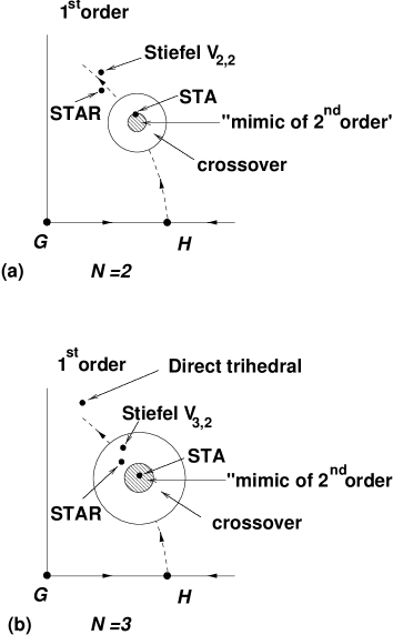
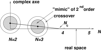
Figure 11: Hypothesis on the Hamiltonian flow induced by renormalization–group transformations for $N<N_{c}$ (see Fig. 2 c) showing the smaller influence of the complex fixed point for the $XY$ spins ($N\!\!=\!2$) compared to the Heisenberg spins ($N\!\!=\!3$). The arrows give the direction of flow and the black circles indicate the positions accessible for the different systems in simulations or experiments. The hatched region is under the influence of the complex fixed point and the outer circle represents the crossover to the first order region.

Figure 12: The position of the fixed point $F_{+}$ as function of $N$ for $d=3$ with its different basins of attraction.

A negative value of $\eta$ is impossible, for a second order phase transition it should always be positive [11]. A slightly negative value was already discernible in some of the results of the unconstrained STA–model, see table 1. In making use of our previous analysis of the $x$–$y$ case [13] we conclude that the critical behavior should be described by the renormalization flow of a fixed point in the complex parameter space. The scaling relation for $\eta$ above is then modified to give a positive value for this critical exponent, see previous section. Moreover this large negative value cannot come from only the presence of a complex fixed point. Thus we interpret the negative value as a crossover from the basin of attraction of the complex fixed point to the true first order transition, see Fig. 12

In a previous study of the STAR model, Dobry and Diep [46] obtained for the exponent $\nu=0.440(20)$ which disagrees with ours 0.504(10). However this seems to be a misprint since the inverse value is also given and $\nu=1/2.08=0.48$ is within the statistical errors. However the other exponents seem wrong. We repeated these calculations for larger clusters and with better statistics in order to have evidence that this system shows a weak first order transition, since unambiguously $\eta$ is really negative

5.2 Stiefel’s $V_{3,2}$ model

Following the same procedure as for the STAR model we determine first $T_{c}$. The cumulant $U$ plotted as a function of temperature for different system sizes from $L=15$ to $L=40$ is shown in Fig.8. The extrapolation, shown in Fig. 8, for $L=20$ and $L=25$ agrees rather well; the little difference for $L=15$ indicates that this lattice size is not yet sufficient for a strictly linear extrapolation. We obtain

$$T_{c}=1.5312(1)$$ (39)

and for the universal quantity $U$ at $T_{c}$

$$U^{*}=0.6326(12).$$ (40)

In plotting the logarithm of $V_{1}$, $\chi_{2}$, $\chi_{4}$ and $\bar{M}$ as function of the logarithm of temperature difference $(T-T_{c})/T_{c}$, shown in Fig. 10, one finds from the slope

$$\nu = 0.507(8)$$ (41)

$$\gamma/\nu = 2.240(10)$$ (42)

$$\gamma_{4}/\nu = 7.480(22)$$ (43)

$$\beta/\nu = 0.381(6).$$ (44)

From $\gamma_{4}/\nu$ using (29) we get $\gamma/\nu=2.240(11)$ which is the same value found directly from $\chi_{2}$. Further we obtain for $\beta=0.193(4)$ and $\gamma=1.136(23)$ and with the scaling relation (38) an even more negative value $\eta=-0.240(10)$. See for a listing table 4, where also the specific heat exponent $\alpha=2-d\nu$ has been added. The errors given include the uncertainty of the estimate of $T_{c}$.

The results of Kunz and Zumbach [15] are also given there and are compatible with ours. Their $\alpha$ is actually determined by fitting specific heat data in the high temperature region and $\nu$ with the hyperscaling relation. They noticed also that $\eta$ is negative, apparently their value $-0.10(5)$ is too small, compared to $-0.24(1)$ we found. We cannot share their conclusion that the negative $\eta$ is due to a strong finite size effect not properly taken care of. We rather take it as an indication that an analysis as a genuine second order transition leads to inconsistencies and interpret the negative value as a crossover from the basin of attraction of the complex fixed point to the true first order transition, see Fig. 12.

5.3 Direct trihedral model

It is known from [37] that the energy distribution $P(E)$ near the critical temperature has a double peak structure. A rough estimate of the correlation length $\xi_{0}$ by $1\over 3$ of the smallest size where the two peaks are well separated by a region of zero probability gives $\xi_{0}=6$. Here we determine the energy cumulant at the transition. Extrapolating $W$ to a system of infinite size we obtain

$$W^{*}\,=\,0.623(1)$$ (45)

which of course deviates from the value $2\over 3$ for a second order transition. It is not difficult to see hysteresis effects. In Fig. 10 hysteresis for the energy $E$ is clearly visible.

Therefore the behavior of a system of trihedrals differs from the one of dihedrals. In weakening the interaction between the third components of the trihedrals one could of course recover the apparent second order nature of the dihedral system. The first order character of the transition of pure dihedrals is impossible to show directly. This system remains always under the influence of the virtual or complex fixed point for the sizes of systems one can simulate, while the presence of the third vector allows the system of trihedrals to stay outside of the neighborhood of this fixed point and the “true” first order behavior is seen directly.

6 Discussion

6.1 Summary

The STAR and the Stiefel model $V_{3,2}$ have slightly different critical exponents. Looking at table 4, most noticeable are the differences for $\beta$ and $\gamma$: $\beta_{STAR}=0.221(9)$ and $\beta_{Stie}=0.193(4)$, outside the estimated statistical and systematic errors. The difference to the values of $\beta\approx 0.286$ for the original stacked triangular antiferromagnet in table 1 is even larger. Also the non–collinear antiferromagnet on the bct lattice has a different $\beta$–value (see table 1). Using the scaling relation $\eta=2-d+2\,\beta/\nu$ the exponent $\eta$ is always negative. Moreover, a member of the same universality class, the right handed trihedral model, has a strong first order transition. This does not correspond to the standard behavior of a universality class one expects from the seemingly clear evidence for a second order transition as visible in Fig. 10 for the STAR and the Stiefel model.

In taking the point of view that the simulations show an extremely weak first order transition it is very natural to use a field theoretical description with the usual renormalization group scheme supplemented by complex fixed points, see Fig. 2. Such complex fixed points exist if the number of components $N$ is lower than a critical one $N_{c}$, and according to field theoretical analysis the critical dimension is $N_{c}\approx 4$. As for a real fixed point the renormalization flow will be attracted and the system imitates a second order behavior, however it can escape if the system size $L$ is larger than the largest correlation length $\xi_{0}$ possible and then the crossover to first order region is reached. This crossover phenomenon is known to occur in the two dimensional Potts model with $q=5$ components [47, 48].

In the analysis based on complex fixed points Zumbach [14] showed that the scaling relations should be modified by correction terms eqs. (4-5). Leaving out these terms the scaling relations for $\eta$ produces negative values, for $XY$ spins of the STA model it is slightly negative ($\eta\sim-0.06$ [13]) and for the models studied here the effect is two or three times larger, see table 4. Another possibility of obtaining negative values for $\eta$ is to visualize the spin system in the crossover region between a second to first order transition. Using the same scaling relations as before the exponent $\eta$ will tend to the value $\eta=-1$ of a “weak first order transition” (table 3). Our MC simulations of the STAR and the Stiefel model are in such a crossover region otherwise the very negative values for $\eta\approx-0.2$ cannot be understood. The same applies for MC simulations of helimagnetics on bct lattices [8].

In contrast to the $XY$ case with $N=2$ the frustrated Heisenberg case is closer to the critical dimension. That is, the STAR and the Stiefel model appear at first sight as second order transitions whereas in the $XY$ case they show really first order behavior [13]. The stacked triangular antiferromagnet STA follows the same trend with a small negative $\eta$ in the $XY$ case and an only slightly negative one in the Heisenberg case table 1. The smaller sphere of influence or basin of attraction of the complex fixed point in the $XY$ case compared to the Heisenberg case is depicted in Fig. 12 and Fig. 12.

Another interpretation following Kawamura [49] takes the diagram in Fig. 2a as basis, where an attractive $F_{+}$ and an unstable fixed point $F_{-}$ are neighbors. The initial points in the RG flow for the STAR and the Stiefel model are placed outside the domain of attraction of the fixed point $F_{+}$, that is, to the left of the line ($G,F_{-}$) in Fig. 2a while the STA model should be to the right of this line. Therefore the STAR and the dihedral model have a first order transition and the STA model a standard second order transition. The difficulty is the critical dimension $N_{c}>3$ according to Antonenko and Sokolov [10] and actually Fig 2c should be the starting point. Beyond all question is that all the MC simulations give a negative $\eta$ impossible to explain with a real fixed point [11]. One observes also the experimental crossover behavior from second order to first order in systems belonging to the $XY$ class like the holmium, dysprosium or $CsCuCl_{3}$ (see [13]) which is in disfavor of this interpretation.

6.2 Experiments

In real systems because of the omnipresence of planar or axial anisotropies the behavior of frustrated Heisenberg antiferromagnets will be difficult to observe. Moreover such systems are usually quasi one or two dimensional, that is a succession of crossovers will occur from 2d to 3d and from Heisenberg to Ising or $XY$ behavior. To observe the first order behavior the temperature must be very close to the critical temperature in order to notice that the correlation length is limited in the basin of attraction of the complex fixed point $F$. For $XY$ spin systems, in spite of this limitation the crossover has been observed in certain materials like Ho [50], Dy [51, 52], CuCoCl₃ [53] (see also [13]).

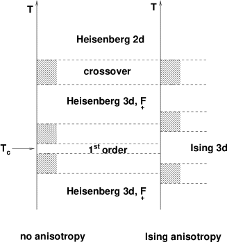
Figure 13: Crossover phenomena in experimental systems (not to scale). There is a crossover to Ising behavior before reaching the first order region. $F_{+}$ indicates that the behavior is caused by the complex fixed point. For real systems it is possible to have other crossover behaviors due to lattice distortions and Dzyaloshinsky-Moriya interactions.

Before the first order region is reached in Heisenberg systems the crossover to Ising or $XY$ behavior prevents a first order transition of Heisenberg type. In Fig. 13 a typical scheme is drawn for the crossovers and transitions of a system with Ising anisotropy, for more details see [1] and for other crossovers [54].

Nevertheless the second order transition can be studied. A list of results is in Table 2: for VCl₂ [55], for VBr₂ [56], for Cu(HCOO)₂2CO(ND₂)₂2D₂O [57] and for Fe[S₂CN(C₂H₅)₂]₂Cl [58]. For the last two examples the observed exponents might be influenced by the crossover between 2d to 3d Ising behavior. The experimental results agree quite well with the MC simulation in table 1.

6.3 Renormalization group studies in 2+$\epsilon$

For the STA model studied in $d=2+\epsilon$ expansion using the corresponding nonlinear $\sigma$–model Azaria et al. [35, 36] obtained for all $N$ a stable fixed point $F_{2+\epsilon}$ at a small distance $\epsilon$ from $d=2$. In comparing results in lowest order of $1/N$ for the $2+\epsilon$ to the $4-\epsilon$ expansion they show that the fixed points found in the different approaches are equivalent for large $N$.

Specially for $N=3$ a clear evidence by symmetry arguments can be given that the transition near $d=2$ should be of the standard ferromagnetic $O(4)$ class. If the transition is of second order also for $d=3$ it must therefore belong to the $O(4)$ class with the exponent $\gamma_{O4}=1.54$ (table 3) very different from the value of the STA model $\gamma_{STA}=1.18$ found by the MC method (table 1). This is not compatible with the Monte Carlo simulations and experimental studies (see tables).

We think that we can rule out the possibility of a ferromagnetic $O(4)$ class for $N=3$ if the relevant operators are the same for large and low $N$. The $1/N$ expansion for $\gamma$ (similar arguments hold for all exponents) for both the ferromagnetic non frustrated (NF) [60] case and frustrated case (F) [2] are:

$$\gamma_{NF} = {2\over d-2}\,\Bigl{[}\,1-{6\over N}\,S_{d}\,\Bigr{]}$$ (46)

$$\gamma_{F} = {2\over d-2}\,\Bigl{[}\,1-{9\over N}\,S_{d}\,\Bigr{]}$$ (47)

where

$$S_{d}={\sin(\pi\,(d-2)/2)\,\Gamma(d-1)\over 2\,\pi\,\Gamma(d/2)^{2}}$$ (48)

is a positive quantity. Thus for $N$ large $\gamma_{NF}>\gamma_{F}$. The reason is the different breakdown of symmetry from $O(N)$ to $O(N-P)$ with $P=1$ in the ferromagnetic case and $P=2$ in the frustrated case. When $N$ decreases the ratio $P/N$ increases also the difference between $\gamma_{NF}$ and $\gamma_{F}$ will increase and one should have $\gamma_{NF}>\gamma_{F}$ for any $N$ and in particular for $N=3$.

However it is possible that irrelevant operators in the $4-\epsilon$ and $1/N$ expansions become relevant near dimension two and low $N$. In this case for $N=3$ the transition should be of first order for dimension three and a little less than three. Below this limit the transition could be of the ”chiral” universality class and in approaching two dimensions it should become a $O_{4}$ transition. This hypothesis has found some support [61]. We note that at exactly two dimensions, systems are known to be driven by the $O(4)$ symmetry, at least at low temperature [62].

Other RG studies near two dimensions [63, 64] have found more than a single transition governed by the $O(4)$ fixed point with an intermediate “nematic” phase between the disordered high temperature region and the ordered $120^{\circ}$ structure at low temperatures. This double transition should also occur for the right handed trihedral model studied here when the interaction between the third components are larger than between the two others. The ordering of the third vector occurs before the ordering of the other two vectors and both transitions are of second order, the first of Heisenberg type and the second of $XY$ type. The intermediate “nematic” phase can also be interpreted as a ferromagnetic phase and the two transitions characterized as paramagnetic–collinear and collinear–noncollinear.

Another possibility discussed in the literature is that the transition is influenced by the presence of topological defects which are not visible in the continuum and perturbation theory as in RG ($2+\epsilon$, $4-\epsilon$ and directly in $d=3$) [62]. In this work we have assumed that the effects of topological defects are irrelevant for the critical behavior [15, 65].

7 Conclusion

We have tried to discuss the phase transition of frustrated Heisenberg spin systems in general terms. The starting point is Monte Carlo simulations of systems for which the condition of local rigidity is imposed. From the finite size analysis we suggest that the transition is of first order. Our result is that one can rely on the renormalization group studies and the true behavior is indeed first order. However one should use the concept of complex fixed points to describe the almost second order behavior of frustrated Heisenberg spin systems. In the strict sense there is no “chiral universality class” but in practical terms it exists. We have given reasons why in the usual Monte Carlo simulations and in experiments this first order transition is difficult or even impossible to observe.

8 Acknowledgments

This work was supported by the Alexander von Humboldt Foundation. The authors are grateful to Professors B. Delamotte, G. Zumbach, H.T. Diep, A. Dobry, Y. Holovatch and F. Nogueira for discussions. We thank A.I. Sokolov, E. Brezin and J. Zinn-Justin for the reference of the proof of $\eta\geq 0$, S. Thoms for the reference of the two loop order calculation for superconductors and A. Schakel for the reference of the gauge dependence of $\eta$ for superconductors. Moreover we want to acknowledge L. Beierlein and M.E. Myer to a carefully reading of the manuscript.

system	ref.	$\alpha$	$\beta$	$\gamma$	$\nu$	$\eta$
STA	[3]	0.240(80)	0.300(20)	1.170(70)	0.590(20)	+0.020(180)1
STA	[4]	0.242(24)2	0.285(11)	1.185(3)	0.586(8)	-0.033(19)1
STA	[6]	0.245(27)2	0.289(15)	1.176(26)	0.585(9)	-0.011(14)1
STA	[5]	0.230(30)2	0.280(15)		0.590(10)	0.000(40)3
bct	[8]	0.287(30)2	0.247(10)	1.217(32)	0.571(10)	-0.131(18)1

Table 1: Critical exponents by Monte Carlo for $O(3)$. STA = stacked triangular antiferromagnet, bct = body-centered-tetragonal, calculated by ${}^{1)}\;\gamma/\nu=2-\eta\,$, ${}^{2)}\;d\nu=2-\alpha\,$, ${}^{3)}\;2\,\beta/\nu=d-2+\eta\,$.

Crystal	method	ref.	$\alpha$	$\beta$	$\gamma$	$\nu$
VCl2	Neutron	[55]		0.20(2)	1.05(3)	0.62(5)
VBr2	Calorimetry	[56]	0.30(5)
CuFUD1	Neutron	[57]		0.22(2)
Insulating2	Neutron	[58]		0.24(1)	1.16(3)

Table 2: Experimental values of critical exponents for compound VCl₂, VBr₂, ¹Cu(HCOO)₂2CO(ND₂)₂2D₂O and ²Fe[S₂CN(C₂H₅)₂]₂Cl.

symmetry	$\alpha$	$\beta$	$\gamma$	$\nu$	$\eta$
$Z_{2}$	0.107	0.327	1.239	0.631	0.038
$SO(2)$	-0.010	0.348	1.315	0.670	0.039
$SO(3)/SO(2)$	-0.117	0.366	1.386	0.706	0.038
$SO(4)/SO(3)$	-0.213	0.382	1.449	0.738	0.036
1$st$ order1	1	0	1	1/3	-12

Table 3: Critical exponents for the ferromagnetic systems calculated by RG [66]. ¹We cannot define exponents in a first order transition, however in the case of a weak first order transition the exponents found in MC and in experiments must tend to these values. ²calculated by $\gamma/\nu=2-\eta$.

system	ref.	$\alpha$	$\beta$	$\gamma$	$\nu$	$\eta$	$T_{c}$
STAR	–	0.488(30)2	0.221(9)	1.074(29)	0.504(10)	-0.131(13)1	1.43122(12)
$V_{3,2}$	–	0.479(24)2	0.193(4)	1.136(23)	0.507(8)	-0.240(10)1	1.5312(1)
$V_{3,2}$	[15]	0.460(30)		1.100(100)	0.515(10)	-0.100(50)	1.532

Table 4: Critical exponents by Monte Carlo for the STAR and the Stiefel model $V_{3,2}$. ¹calculated by $\gamma/\nu=2-\eta$. ²calculated by $d\nu=2-\alpha$.

Figure 5: Binder’s parameter $U$ for the STAR model as function of the temperature for different sizes $L$ (in the left part of the figure upwards from $L$=18 to $L$=42). The arrow indicates the critical temperature $T_{c}$.

Figure 6: Estimated $T_{c}$ for the STAR model plotted vs inverse logarithm of the scale factor $b=L^{\prime}/L$ . For clarity, only the results for $L$=18, 21, 24 are shown. The estimated temperature is $T_{c}$=1.43122(12).

Figure 7: Binder’s parameter $U$ for Stiefel’s model $V_{3,2}:$ as function of temperature for different sizes $L$ (in the left part of the figure upwards from $L=15$ to $L=40$). The arrow indicates the critical temperature $T_{c}$.

Figure 8: Estimated $T_{c}$ for the Stiefel model $V_{3,2}:$ plotted vs inverse logarithm of the scale factor $b=L^{\prime}/L\,$. For clarity, only the results for $L=15,\,20,\,25$ are shown. The estimated temperature is $T_{c}$=1.5312(1).

Figure 9: Values of $\chi_{2}$, $V_{1}$ and $\bar{M}$ as function of $L$ in ln–ln scale at $T_{c}$ for the STAR and the Stiefel model $V_{3,2}:$ to get the slopes $\gamma/\nu$, $1/\nu$ and $\beta/\nu$. Error bars are smaller than symbols. To obtain a clear figure values for $\bar{M}$ are shifted by +3 units.

Figure 10: Hysteresis in the internal energy per spin $E$ versus T for the right handed trihedral system. Lines are guides to the eye. The arrows indicate if the MC simulation is cooling (circle) or heating (square) the system.

References

- [1] Magnetic Systems with Competing Interactions (Frustrated Spin Systems), edited by H.T. Diep (World Scientific, Singapore, 1994).
- [2] H. Kawamura, Phys. Rev. B 38, 4916(1988), 42, 2610 (1990).
- [3] H. Kawamura, J. Phys. Soc. Jpn 61, 1299 (1992), 56,474 (1987), 54, 3220 (1985).
- [4] M.L. Plumer and A. Mailhot, Phys. Rev. B 50, 6854 (1994).
- [5] D. Loison and H.T. Diep, Phys. Rev. B 50, 16453 (1994).
- [6] T. Bhattacharya, A. Billoire, R. Lacaze and Th. Jolicoeur, J. Phys. I (Paris) 4, 181 (1994).
- [7] H.T. Diep, Phys. Rev. B 39, 397 (1989)
- [8] D. Loison, in preparation
- [9] S.A. Antonenko, A.I. Sokolov and V.B. Varnashev, Phys. Lett. A 208, 161 (1995).
- [10] S.A. Antonenko and A.I. Sokolov, Phys. Rev. B 49 15901(1994).
- [11] A.Z. Patashinskii and V.I. Pokrovskii, Fluctuation Theory of Phase Transitions, (Pergamon press 1979), §VII, 6 , The S-matrix method and unitary relations.
- [12] J. Zinn-Justin, Quantum Field Theory and Critical Phenomena, (Oxford University Press, Oxford, 1996), §7.4 Real-time quantum field theory and S-matrix, §11.8 Dimensional regularization, minimal subtraction: calculation of RG functions.
- [13] D. Loison and K.D. Schotte, Eur. Phys. J. B 5, 735 (1998)
- [14] G. Zumbach, Phys. Rev. Lett. 71, 2421 (1993), Nucl. Phys. B 413,771 (1994).
- [15] H. Kunz and G. Zumbach,J. Phys. A 26, 3121 (1993).
- [16] D. Bailin, A. Love, and M.A. Moore, J. Phys. C 10, 1159 (1977).
- [17] D.R.T. Jones, A. Love, and M.A. Moore, J. Phys. C 9, 743 (1976).
- [18] T. Garel and P. Pfeuty, J. Phys. C 9, L245 (1976).
- [19] We thank A.I. Sokolov for this comment.
- [20] J.C. Le Guillou and J. Zinn-Justin, J. Phys. (Paris) Lett. 46, L137 (1985)
- [21] B.I. Halperin, T.C. Lubensky and S.K. Ma, Phys. Rev. Lett. 32, 292 (1974).
- [22] J-H. Chen, T.C. Lubensky and D.R. Nelson, Phys. Rev. B 17, 4274 (1978).
- [23] J.P. Tessmann, Diplomarbeit, Freie Universität Berlin, 1984, ”Two loop Renormierung der Skalaren Elektrodynamik”, unpublished.
- [24] P.G. De Gennes, Solid State Commun. 10, 753 (1972).
- [25] B.I. Halperin and T.C. Lubensky, Solid State Commun. 14, 997 (1974).
- [26] B.R. Patton and B.S. Andereck, Phys. Rev. Lett. 69, 1556 (1992), L. Chen, J.D. Brock and J. Huang and S. Kumar, Phys. Rev. Lett. 67, 2037 (1991) and references therein.
- [27] M. Kiometzis and A. M. J. Schakel, Int. J. Mod. Phys. B 7, 4271 (1993).
- [28] A.B. Harris, T.C. Lubensky, J.H. Chen, Phys. Rev. Lett. 36, 415 (1976).
- [29] A. N. Vasil’ev and M. Yu. Nalimov, Teor. Mat. Fiz. 56, 15 (1983).
- [30] F. S. Nogueira, cond-mat/9808097
- [31] G. Zumbach, Nucl. Phys. B 413, 754 (1994).
- [32] U. Wolff, Phys. Rev. Lett. 62, 361 (1989), Nucl. Phys. B 322, 759 (1989)
- [33] U. Wolff, Phys. Lett. B 228, 379 (1989), W. Janke, Phys. Lett. A 148, 306 (1990), J.S. Wang, Physica A 164, 240 (1990)
- [34] A.D. Sokal, S. Caracciolo, R.G. Edwards and A. Pelisseto, Nucl. Phys. B (proc. Suppl.) 20, 55, 72 (1991), 26, 595 (1992)
- [35] P. Azaria and B. Delamotte, in [1].
- [36] P. Azaria, B. Delamotte,F. Delduc and T. Jolicoeur, Nucl. Phys. B 408, 485 (1993), P. Azaria, B. Delamotte and T. Jolicoeur, Phys. Rev. Lett. 64, 3175 (1990), J. App. Phys. 69, 6170 (1991).
- [37] D. Loison, H.T. Diep, J. Appl. Phys. 76, 6350 (1994)
- [38] A. M. Ferrenberg and R. H. Swendsen, Phys. Rev. Let. 61, 2635 (1988), Phys. Rev. Let. 63, 1195 (1989).
- [39] B. Efron, The Jackknife, The Bootstrap and other Resampling Plans (SIAM, Philadelphia, PA, 1982)
- [40] Barber, in Phase Transition and Critical Phenomena, edited by C. Domb and J.L. Lebowitz (Academic, New York, 1983), Vol. 8
- [41] A. M. Ferrenberg and D. P. Landau, Phys. Rev. B 44, 5081 (1991)
- [42] K. Binder, Z. Phys. B 43, 119 (1981)
- [43] V. Privman and M.E. Fisher, J. Stat. Phys. 33, 385 (1983).
- [44] K. Binder, Rep. Prog. Phys. 50, 783 (1987)
- [45] A. Billoire, R Lacaze and A. Morel, Nucl. Phys. B 370 773 (1992).
- [46] A. Dobry and H.T. Diep, Phys. Rev. B 51, 6731 (1995).
- [47] R.J. Baxter, Exactly solved models in statistical mechanics (Academic Press, London, 1982).
- [48] P. Peczak and D.P. Landau, Phys. Rev. B 39, 11 932 (1989).
- [49] H. Kawamura, Cond. Matter 10 4708 (1998)
- [50] D.A. Tindall, M.O. Steinitz and M.L. Plumer, J. Phys. F 7, L263 (1977).
- [51] S.W. Zochowski, D.A. Tindall, M. Kahrizi, J. Genosser and M.O. Steinitz, J. Magn. Magn. Mater. 54-57, 707 (1986).
- [52] H.U. Åström and G. Benediktson, J. Phys. F 18, 2113 (1988).
- [53] H. B. Weber, T. Werner, J. Wosnitza H.v. Löhneysen and U. Schotte, Phys. Rev. B 54, 15924 (1996).
- [54] M.F. Collins, O.A. Petrenko, Can. J. Phys. 75, 605 (1997)
- [55] H. Kadowaki, K. Ubukoshi, K. Hirakawa, J.L. Martinez and G. Shirane, J. Phys. Soc. Japan 56, 4027 (1987).
- [56] J. Wosnitza, R. Deutschmann, H.v Löhneysen and R.K. Kremer, J. Phys.: Condens. Matter 6, 8045 (1994).
- [57] K. Koyama and M. Matsuura, J. Phys. Soc. Japan 54, 4085 (1985)
- [58] G.C. DeFotis, F. Palacio and R.L. Carlin, Physica B 95, 380 (1978), G.C. DeFotis and S.A. Pugh, Phys. Rev. B 24, 6497 (1981), G.C. DeFotis and J.R. Laughlin, J. Magn. Magn. Mater. 54-57, 713 (1986).
- [59] T.R. Thurston, G. Helgesen, D. Gibbs, J.P. Hill, B.D. Gaulin and G. Shirane, Phys. Rev. Lett. 70, 3151 (1993) , T.R. Thurston, G. Helgesen,J.P. Hill, D. Gibbs, B.D. Gaulin and P.J. Simpson, Phys. Rev. B 49, 15730 (1994).
- [60] S.K. Ma, Phys. Rev. A 7, 2172 (1973)
- [61] B. Delamotte, D. Mouhanna, P. Lecheminant Phys. Rev. B 59, 6006 (1999).
- [62] B.W. Southern and A.P. Young, Phys. Rev. B 48, 13170 (1993), M. Wintel, H.U. Everts and W. Apel Phys. Rev. B 52, 13480 (1995).
- [63] F. David and T. Jolicoeur, Phys. Rev. Lett. 76,3148 (1996).
- [64] A. V. Chubukov, Phys. Rev. B 44, 5362(1991).
- [65] G. Zumbach, Phys. Lett. A 200, 257 (1995).
- [66] S.A. Antonenko, A.I. Sokolov, Phys. Rev. E 51, 1894 (1995).