Chaos, Dissipation and Quantal Brownian Motion
(Lecture notes of course in the international school of physics Enrico Fermi,
Session CXLIII New Directions in Quantum Chaos, Varenna Italy, July 1999)

Abstract

Quantum dissipation, the theory of energy spreading and quantal Brownian motion are considered. In the first part of these lecture-notes we discuss the classical theory of a particle that interacts with chaotic degrees of freedom:
$\bullet\$The Sudden and the Adiabatic approximations;
$\bullet\$The route to stochastic behavior;
$\bullet\$The fluctuation-dissipation relation;
$\bullet\$And the application to the ‘piston’ example.

In the second part of these lecture-notes we discuss the restricted problem of classical particle that interacts with quantal (chaotic) degrees of freedom:
$\bullet\$Limitations on quantal-classical correspondence;
$\bullet\$The perturbative core-tail spreading profile;
$\bullet\$Linear response theory versus Fermi-golden-rule picture;
$\bullet\$Random-matrix-theory considerations;
$\bullet\$And the quantal Sudden and Adiabatic approximations.

In the third part of these lecture-notes we discuss the problem of quantal particle that interacts with an effective harmonic bath:
$\bullet\$Classical Brownian motion;
$\bullet\$The ZCL model and the DLD model;
$\bullet\$The white noise approximation;
$\bullet\$The reduced propagator and master-equation formulation;
$\bullet\$And the two mechanisms for dephasing.

We conclude with explaining the main open question in the theory of quantum dissipation and quantal Brownian motion. That question concerns the problem of quantal particle that interacts with quantal (chaotic) degrees of freedom.

1 Definition of the problem

We are interested in the reduced dynamics of a slow degree of freedom $({\mathbf{x}},{\mathbf{p}})$ that interacts with a ‘bath’. The Hamiltonian is

$${\cal H}\ =\ {\cal H}_{0}({\mathbf{x}},{\mathbf{p}})+{\cal H}_{\mbox{\tiny env}}({\mathbf{x}},Q_{\alpha},P_{\alpha})$$ (1)

In Fig.1 we display a list of our main assumptions and an illustration of our leading example. In this example the slow degree of freedom is the ‘piston’, and the ‘bath’ consist of one gas particle.

Assumptions:
$\bullet$   ${\cal H}_{\mbox{\tiny env}}(Q,P;{\mathbf{x}})$ with ${\mathbf{x}}{=}\mbox{const}$ generates classically chaotic dynamics.
$\bullet$   ${\cal H}_{0}({\mathbf{x}},{\mathbf{p}})={\mathbf{p}}^{2}/(2m)$ describes a free particle. (optional is linear driving).
$\bullet$   Initially the bath is characterized either by an energy $E$ or by a temperature $T$.
$\bullet$   In a classical sense ${\mathbf{x}}(t)$ is a slow degree of freedom.

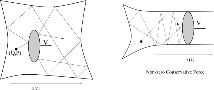
Figure 1: List of main assumptions and an illustration of the ‘piston’ example.

Classically the reduced dynamics of the slow degree of freedom is described by the Langevin equation

$$m\ddot{{\mathbf{x}}}\ =\ {\cal F}(t)$$ (2)

where ${\cal F}(t)$ is a stochastic force. The average force on the particle is

$$\langle{\cal F}(t)\rangle\ =\ F({\mathbf{x}})-\mu\dot{{\mathbf{x}}}$$ (3)

Without loss of generality, just for the sake of simplicity, we assume from now on that the velocity-independent force $F({\mathbf{x}})$ is equal to zero (see Fig.1). Thus there is no reversible energy change due to conservative work. However, there is still systematic irreversible change of energy due to the friction force. The energy dissipation rate is:

$$\frac{d}{dt}\left\langle\ \frac{1}{2}m\dot{{\mathbf{x}}}^{2}\right\rangle\ \approx\ -\mu\dot{{\mathbf{x}}}^{2}\ \ \ \ \ \mbox{for non-thermal motion.}$$ (4)

The fluctuating component of the stochastic force is like white noise, and it is characterized by its intensity $\nu$. The dissipation constant $\mu$ is related to the noise intensity $\nu$ via a universal Fluctuation-Dissipation (FD) relation

$$\mu\ =\ \frac{\nu}{2k_{\mbox{\tiny B}}T}$$ (5)

We are interested in developing a corresponding quantum mechanical theory of dissipation and quantal Brownian motion. ‘Dissipation’ means from now on that energy is absorbed by the bath degrees of freedom due to the time dependence of ${\mathbf{x}}$. The dissipation coefficient is $\mu$. ‘Brownian motion’ refers from now on to the reduced dynamics of the $({\mathbf{x}},{\mathbf{p}})$ degree of freedom. We shall use the term ‘piston’ rather than ‘Brownian particle’ if the motion is constrained to one dimension. Note that the term ‘piston’ is not used in its literal sense.

2 Restricted versions of the problem

The quantum mechanical treatment of the general problem is extremely complicated. Therefore it is a good idea to analyze restricted versions of the general problem. Treating ${\mathbf{x}}(t)$ as a classical degree of freedom, we can consider the time dependent Hamiltonian

$${\cal H}\ =\ {\cal H}_{\mbox{\tiny env}}(Q,P;{\mathbf{x}}(t))$$ (6)

For simplicity we can further assume that ${\mathbf{x}}(t)$ describes a motion with a constant velocity $\dot{{\mathbf{x}}}=V$. Consequently we can treat $x$ in (6) as a one-degree-of-freedom variable. This restricted problem is the main issue of the following lectures (parts 1 and 2).

In consistency with the terminology that has been introduced at the end of the previous section, we shall refer to the restricted problem defined above as ‘the problem of quantum dissipation’. Obviously, in other physical examples $x$ does not have to be the position of a particle. It can be any controlling parameter that appears in the Hamiltonian, e.g. electric field. Of particular interest is the case where $x$ is the magnetic flux via a ring. The velocity $V=\dot{x}$ has then the meaning of electro-motive-force. Let us assume that the ring contains one charged particle $(Q,P)$ that performs diffusive motion. The charged particle gains kinetic energy, and the dissipation coefficient $\mu$ is just the conductivity of the ring. Note that in actual circumstances the charged-particle is an electron, and its (increasing) kinetic energy is eventually transfered to the vibrational modes (phonons) of the ring, leading to Joule heating. The latter process is ‘on top’ of the generic dissipation problem that we are going to analyze.

We come back to the Brownian particle / ‘piston’ example, and shift the focus from the ‘bath’ to the reduced-dynamics of the $({\mathbf{x}},{\mathbf{p}})$ degree-of-freedom. We can study the effect of the fluctuating force by considering an Hamiltonian of the type

$${\cal H}\ =\ \frac{{\mathbf{p}}^{2}}{2m}+{\cal U}({\mathbf{x}},t)$$ (7)

where ${\cal U}({\mathbf{x}},t)$ is an effective stochastic potential the mimics the noisy character of the environment. Obviously, with such Hamiltonian we cannot mimic the effect of dissipation. In order to have dissipation the interaction should be with dynamical degrees of freedom. We can introduce an effective harmonic-bath as follows:

$${\cal H}\ =\ \frac{{\mathbf{p}}^{2}}{2m}\ -\ \sum_{\alpha}c_{\alpha}Q_{\alpha}u({\mathbf{x}}{-}{\mathbf{x}}_{\alpha})\ +\ \sum_{\alpha}\left(\frac{P_{\alpha}^{2}}{2m_{\alpha}}+\frac{1}{2}m\omega_{\alpha}^{2}Q_{\alpha}^{2}\right)$$ (8)

The effective-noise model (7) as well as the effective harmonic-bath model (8) can be treated analytically using the Feynman-Vernon (FV) formalism. The reduced dynamics of the particle is obtained after averaging over realizations of the stochastic potential (in case of (7)), or by elimination of the environmental degrees of freedom (in case of (8)). It leads to a unified description of diffusion localization and dissipation (DLD). It is found indeed that the formal solution of (8) reduces to that of (7) if dissipation effect is neglected. We shall refer to (8), and more generally to its formal solution, as the ‘DLD model’. It is possible to introduce an effective RMT-bath instead of an effective harmonic bath, but then there is no general analytical solution. It has been demonstrated however that at high temperatures an approximate treatment of the effective RMT-bath coincides with the exact (high temperature) solution of the DLD model.

3 ‘History’ of the problem (possibly biased point of view [1])

There is a well established classical theory for dissipation and Brownian motion. In the pre-chaos literature (${\sim}1980$) the dissipation constant for a moving ‘piston’ is given by the ‘wall formula’. See [4, 5] and followers. A more general point of view, which is discussed in the first part of these lectures (Sections 4-11), has been adopted in the post-chaos literature (${\sim}1990$). There, the emphasis is on relating the dissipation constant to the intensity of fluctuations [14, 15, 17, 18].

Various methods such as ‘linear response’, ‘Kubo-Greenwood formalism’, and ‘multiple scale analysis’ have been used [5, 15, 18] in order to make a quantum mechanical derivation of the FD relation. All these methods are essentially equivalent to a naive application of the Fermi-Golden-Rule (FGR) picture. The validity of the naive FGR result has been challenged in by Wilkinson and Austin [16]. They came up with a surprising conclusion that we would like to paraphrase as follows: A proper FGR picture, supplemented by an innocent-looking RMT assumption, leads to a modified FGR result; In the classical limit the modified FGR result disagrees with the FD relation and leads to violation of the quantal-classical correspondence principle. Obviously this conclusion should be regarded as a provocation for constructing a proper theory for Quantum Dissipation [19, 20]. This is the issue of the second part of these lectures (Sections 12-24). The theory is strongly related to some studies of parametric dynamics [25, 26, 27, 28] and wavepacket dynamics [29, 30, 31].

Most of the literature that comes under the heading ‘Quantum Dissipation’ is concerned with the more general problem where $x$ is a dynamical variable [12]. A direct handling of the ‘bath’ degrees of freedom is usually avoided. As an exception see for example [13]. It is common to adopt an ‘effective-bath’ approach. See [2, 3, 6] and followers. Specific discussion of quantal Brownian motion has been introduced in [7] and later in [8, 9]. It leads to the DLD model, that unifies the treatment of diffusion localization and dissipation. This is the issue of the third part of these lectures (Sections 25-31). The high temperature version of the DLD model is obtained also by considering coupling to an effective RMT-Bath [10].

4 Fluctuations: intensity and correlation time

We consider the Hamiltonian ${\cal H}(Q,P;x)$ with $x{=}\mbox{const}$. The phase space volume which is enclosed by the energy surface ${\cal H}(Q,P;x)=E$ will be denoted by $\Omega(E;x)$. For the classical density of states we shall use the notation $g(E)=\partial_{\mbox{\tiny E}}\Omega(E)$. We define

$${\cal F}(t)\ =\ -\frac{\partial{\cal H}}{\partial x}(Q(t),P(t);x)$$ (9)

The conservative force $F(x)=\langle{\cal F}(t)\rangle_{\mbox{\tiny E}}$ is obtained by performing microcanonical averaging over $(Q,P)$. It is equal to zero if and only if $\Omega(E;x)$ is independent of $x$. For simplicity we assume from now on that this is indeed the case. Now we define a correlation function

$$C_{\mbox{\tiny E}}(\tau)\ =\ \langle{\cal F}(t){\cal F}(t{+}\tau)\rangle_{\mbox{\tiny E}}$$ (10)

The fluctuating force is characterized by an intensity

$$\nu_{\mbox{\tiny E}}\ =\ \int_{-\infty}^{\infty}C_{\mbox{\tiny E}}(\tau)d\tau$$ (11)

and by a correlation time $\tau_{\mbox{\tiny cl}}$. The power spectrum of the fluctuations $\tilde{C}_{\mbox{\tiny E}}(\omega)$ is the Fourier transform of $C_{\mbox{\tiny E}}(\tau)$. For chaotic bath the stochastic force is like white noise. We always have $\tau_{\mbox{\tiny cl}}\leq t_{\mbox{\tiny erg}}$, where $t_{\mbox{\tiny erg}}$ is the ergodic time. In the general discussion we shall not distinguish between the two time scales. However, in specific examples the distinction is meaningful. For example, in case of the ‘piston’ example $\tau_{\mbox{\tiny cl}}$ is the collision time with the walls of the piston, while $t_{\mbox{\tiny erg}}$ is of the order of the ballistic time $\tau_{\mbox{\tiny bl}}$.

5 Fluctuations: time dependent Hamiltonian

We consider from now on the time-dependent Hamiltonian ${\cal H}(Q,P;x(t))$ with constant non-zero velocity $\dot{x}=V$. We define

$${\cal F}(t)\ =\ -\frac{\partial{\cal H}}{\partial x}(Q(t),P(t);x(t))$$ (12)

The statistical properties of the fluctuating force ${\cal F}(t)$ are expected to be slightly different from the $V{=}0$ case. The average $\langle{\cal F}(t)\rangle$ is no longer expected to be zero. Rather, we expect to have $\langle{\cal F}(t)\rangle=-\mu V$. This implies that the correlator $\langle{\cal F}(t_{1}){\cal F}(t_{2})\rangle$ acquires an offset $(\mu V)^{2}$. We shall argue that if the velocity $V$ is small enough then the ‘offset correction’ can be ignored for a relatively long time which will be denoted by $t_{\mbox{\tiny frc}}$. Obviously it is essential to have

$$\tau_{\mbox{\tiny cl}}\ \ll\ t_{\mbox{\tiny frc}}\ \ \ \ \ \mbox{[non-trivial slowness condition].}$$ (13)

There is another possible reason for the correlator $\langle{\cal F}(t_{1}){\cal F}(t_{2})\rangle$ to be different from $C_{\mbox{\tiny E}}(t_{2}{-}t_{1})$. Loss of correlation may be either due to the dynamics of $(Q(t),P(t))$ or else due to the parametric change of $x(t)$. We can define a parametric correlation scale $\delta x_{c}^{\mbox{\tiny cl}}$. For the piston example it is just the penetration distance into the piston upon collision (the effective ‘thickness’ of the wall). The associated parametric correlation time is $\tau_{c}^{\mbox{\tiny cl}}=\delta x_{c}^{\mbox{\tiny cl}}/V$. We assume that

$$\tau_{\mbox{\tiny cl}}\ \ll\ \tau_{c}^{\mbox{\tiny cl}}\ \ \ \ \ \mbox{[trivial slowness condition].}$$ (14)

meaning that loss of correlations is predominantly determined by the chaotic nature of the dynamics rather than by the (slow) parametric change of the Hamiltonian. For the piston example application of the above requirements leads to the obvious condition $V\ll v_{\mbox{\tiny E}}$, where $v_{\mbox{\tiny E}}$ is the velocity of the gas particle.

6 Actual, Parametric and Reduced energy changes

For the time dependent Hamiltonian ${\cal H}(Q,P;x(t))$ energy is not a constant of the motion. Changes in the actual energy ${\cal E}(t)$ reflect ‘real’ dynamical changes as well as parametric changes. Therefore it is useful to introduce the following definitions:

$${\cal E}(t)\ \ =\ {\cal H}(Q(t),P(t);x(t))$$ (15)

$${\cal E}^{\prime}(t)\ =\ {\cal H}(Q(t),P(t);x(0))$$ (16)

The actual energy change can be calculated as follows:

$$\frac{d{\cal E}}{dt}\ =\ \frac{\partial{\cal H}}{\partial t}\ =\ -{\cal F}(t)\cdot V$$ (17)

$$\delta{\cal E}\ =\ {\cal E}(t)-{\cal E}(0)\ =\ -V\int_{0}^{t}{\cal F}(t^{\prime})dt^{\prime}$$ (18)

The actual energy change $\delta{\cal E}$ can be viewed as a sum of parametric-energy-change $\delta{\cal E}_{o}$, and reduced-energy-change $\delta{\cal E}^{\prime}$.

$$\delta{\cal E}\ \ = \ {\cal H}(Q(t),P(t);x(t))-{\cal H}(Q(0),P(0);x(0))$$ (19)

$$\delta{\cal E}_{o}\ = \ {\cal H}(Q(t),P(t);x(t))-{\cal H}(Q(t),P(t);x(0))$$ (20)

$$\delta{\cal E}^{\prime}\ = \ {\cal H}(Q(t),P(t);x(0))-{\cal H}(Q(0),P(0);x(0))$$ (21)

The reduced energy change $\delta{\cal E}^{\prime}$ reflects the deviation of $(Q,P)$ from the original energy surface. It can be calculated as follows:

$$\delta{\cal E}^{\prime}\ =\ V\cdot\left[{\cal F}(t)\times t\ -\ \int_{0}^{t}{\cal F}(t^{\prime})dt^{\prime}\right]$$ (22)

On the other hand, the actual energy change $\delta{\cal E}$ reflects the deviation of $(Q,P)$ from the instantaneous energy surface.

7 The Sudden and the Adiabatic approximations

Figure 2: Schematic illustration of the dynamics. An initially localized distribution is launched in phase space. For a limited time (left plot) it travels upon the initial energy surface. But then it departs from it. After much longer times (right plot) the evolving distribution is concentrated across an instantaneous energy surface.

By inspection of the expressions for the reduced energy change we arrive at the conclusion that for short times we have the so called ‘sudden approximation’:

$$\delta{\cal E}^{\prime}\ \approx\ 0\ \ \ \ \ \mbox{for $t\ll\tau_{\mbox{\tiny cl}}$}$$ (23)

By inspection of the expression for the actual energy change we arrive at the conclusion that for longer times we have the so called ‘adiabatic approximation’:

$$\delta{\cal E}\ \sim\ 0\ \ \ \ \ \mbox{for $t\ll t_{\mbox{\tiny frc}}$}$$ (24)

The time evolution of an initially localized phase-space distribution $\rho_{0}(Q,P)$ is illustrated in Fig.2. For short times we have in general non-stationary time evolution:

$${\cal U}(t)\ \rho_{0}(Q,P)\ \neq\ \rho_{0}(Q,P)\ \ \ \ \ \ \ \ \ \ \ \ \ \ \ \ \mbox{for $t\ll\tau_{\mbox{\tiny cl}}$}$$ (25)

Here ${\cal U}(t)$ is the classical propagator of phase space points. However, if we operate with the same ${\cal U}(t)$ on a microcanonical distribution, then

$${\cal U}(t)\ \rho_{\mbox{\tiny E,x(0)}}(Q,P)\ \approx\ \rho_{\mbox{\tiny E,x(0)}}(Q,P)\ \ \ \ \ \ \ \mbox{for $t\ll\tau_{\mbox{\tiny cl}}$}$$ (26)

It is as if the microcanonical state does not have the time to adjust itself to the changing Hamiltonian. The sudden approximation implies that for short times ${\cal U}(t)$ can be replaced by unity if it operates on an initial microcanonical state. For longer times we have

$${\cal U}(t)\ \rho_{0}(Q,P)\ \sim\ \rho_{\mbox{\tiny E,x(t)}}(Q,P)\ \ \ \ \ \ \ \mbox{for $t_{\mbox{\tiny erg}}\ll t\ll t_{\mbox{\tiny frc}}$}$$ (27)

Here there is enough time for the evolving distribution to adjust itself to the changing Hamiltonian. If we start with a microcanonical state, then the above similarity will hold for any $t\ll t_{\mbox{\tiny frc}}$. The adiabatic approximation becomes worse and worse as time elapses due to the transverse spreading across the energy surface. We shall see that $t_{\mbox{\tiny frc}}$ is the breaktime for the adiabatic approximation.

8 Ballistic and Diffusive energy spreading

We recall the formula for the actual energy change

$${\cal E}(t)-{\cal E}(0)\ =\ -V\int_{0}^{t}{\cal F}(t^{\prime})dt^{\prime}$$ (28)

We Assume an initial microcanonical preparation which is characterized by an energy $E$. The energy spreading after time $t$ is:

$$\langle({\cal E}(t)-{\cal E}(0))^{2}\rangle\ =\ V^{2}\int_{0}^{t}\int_{0}^{t}\langle{\cal F}(t_{1}){\cal F}(t_{2})\rangle\ dt_{1}dt_{2}$$ (29)

Now we make the following approximation

$$\langle{\cal F}(t_{1}){\cal F}(t_{2})\rangle\ \approx\ C_{\mbox{\tiny E}}(\tau)\ \ \ \ \ \ \ \ \ \ \mbox{applicable if $\ t\ll t_{\mbox{\tiny frc}}$}$$ (30)

The validity of this approximation is restricted by the condition $t\ll t_{\mbox{\tiny frc}}$ which will be discussed later. The energy spread is

$$\langle({\cal E}(t)-{\cal E}(0))^{2}\rangle\ \approx\ C_{\mbox{\tiny E}}(0)\cdot(Vt)^{2}\ \ \ \ \ \ \ \ \ \ t\ll\tau_{\mbox{\tiny cl}}$$ for (31)

$$\langle({\cal E}(t)-{\cal E}(0))^{2}\rangle\ \approx\ 2D_{\mbox{\tiny E}}\ t\ \ \ \ \ \ \ \ \ \ \ \ \ \ \ \ \ \ \tau_{\mbox{\tiny cl}}\ll t\ll t_{\mbox{\tiny frc}}$$ for (32)

The ballistic spreading on short time scales just reflects the parametric change of the energy surfaces. The diffusive spreading on longer times reflects the deviation from the adiabatic approximation. The diffusion coefficient is

$$D_{\mbox{\tiny E}}\ \ =\ \ \frac{1}{2}V^{2}\int_{-t}^{t}C_{\mbox{\tiny E}}(\tau)d\tau\ \ \rightarrow\ \ \frac{1}{2}\ \nu_{\mbox{\tiny E}}\ V^{2}$$ (33)

9 Energy spreading and dissipation

It is possible to argue that the energy distribution $\rho(E)$ obeys the following diffusion equation:

$$\frac{\partial\rho}{\partial t}\ =\ \frac{\partial}{\partial E}\left[g(E)D_{\mbox{\tiny E}}\ \frac{\partial}{\partial E}\left(\frac{1}{g(E)}\rho\right)\right]\ \ \ \ \ \ \ \ \mbox{for $t\gg t_{\mbox{\tiny erg}}$}$$ (34)

If we transform to the proper phase space variable $n=\Omega(E)$, this diffusion equation gets the standard form. The average energy is calculated via

$$\langle{\cal E}(t)\rangle=\int_{0}^{\infty}E\ \rho(E)dE$$ (35)

and consequently

$$\frac{d}{dt}\langle{\cal E}\rangle\ =\ -\int_{0}^{\infty}dE\ g(E)D_{\mbox{\tiny E}}\ \frac{\partial}{\partial E}\left(\frac{\rho(E)}{g(E)}\right)\ \ \equiv\ \ \mu V^{2}$$ (36)

Using the expression for $D_{\mbox{\tiny E}}$ We obtain the following FD relation

$$\mu_{\mbox{\tiny E}}\ =\ \frac{1}{2}\frac{1}{g(E)}\frac{\partial}{\partial E}(g(E)\nu_{\mbox{\tiny E}})$$ (37)

The actual value of $\mu$ is obtained by averaging $\mu_{\mbox{\tiny E}}$ according to the distribution $\rho(E)$. The standard version of the FD relation $\mu=\nu/(2k_{\mbox{\tiny B}}T)$ is obtained if $\rho(E)$ is of the canonical type.

10 Application to the ‘piston’ example

It is instructive to apply the FD relation for the ‘piston’ example. The bath degrees of freedom is a gas particle whose mass is $\mathsf{m}$. The faces of the piston are characterized by their total Area. The piston is moving with a constant velocity $V$ inside a $d$-dimensional cavity. For simplicity we treat the collisions as ‘one-dimensional’ and omit $d$ dependent pre-factors [20]. An illustration of one collision with the piston is presented in Fig.3. Each collision can be either from the left or from the right side. The resultant stochastic force which is experienced by the piston is a sum over short impulses:

$${\cal F}(t)\ =\ \sum_{\mbox{\tiny col}}[2\mathsf{m}(v_{\mbox{\tiny col}}-V)]\ \delta(t-t_{\mbox{\tiny col}})$$ (38)

The duration of each impulse is equal to the penetration-time upon a collision with the (soft) faces of the piston. If successive collisions with the piston are uncorrelated, then the correlation time $\tau_{\mbox{\tiny cl}}$ is equal to the average duration of an impulse. The main steps in the analysis of the multi-collision process are summarized in Fig.3 as well. It is easily verified that the FD relation between $\mu_{\mbox{\tiny E}}$ and $\nu_{\mbox{\tiny E}}$ is satisfied. Note however that a proper application of kinetic theory is essential in order to obtain the correct geometrical factors involved [20].

$\bullet$    Assume that the velocities $\ |v_{\mbox{\tiny col}}|\ \sim\ v_{\mbox{\tiny E}}\$ are uncorrelated.
$\bullet$    The average time between collisions is $\tau_{\mbox{\tiny col}}\ =\ (\mbox{\small Volume}/\mbox{\small Area})\ /\ v_{\mbox{\tiny E}}$.
$\bullet$    For $V=0$ we have $\langle{\cal F}(t)\rangle=0$ and $\nu_{\mbox{\tiny E}}=(2\mathsf{m}v_{\mbox{\tiny E}})^{2}\cdot(1/\tau_{\mbox{\tiny col}})$.
$\bullet$    For $V\neq 0$ we have $\langle{\cal F}(t)\rangle=-\mu_{\mbox{\tiny E}}V$ where $\mu_{\mbox{\tiny E}}=2\mathsf{m}\cdot(1/\tau_{\mbox{\tiny col}})$
$\bullet$    The phase space volume is $\Omega(E)=\mbox{\small Volume}\cdot(\mathsf{m}v_{\mbox{\tiny E}})^{d}$.

Figure 3: Illustration of one collision with the piston, and a list of steps in the analysis of a series of such collisions. The Area of the moving faces, the Volume of the cavity, the mass $\mathsf{m}$ of the gas-particle, and its kinetic energy $E$ should be specified. Geometric $d$-dependent prefactors have been dropped. See [20] for exact calculations.

The FD relation is a very powerful tool . This becomes most evident once we consider a variation of the above example: If successive collisions with the piston are correlated, for example due to bouncing behavior, then it is still a relatively easy task to estimate $\nu_{\mbox{\tiny E}}$ for the $V=0$ case, and then to obtain $\mu_{\mbox{\tiny E}}$ via the FD relation. On the other hand, a direct evaluation of $\mu_{\mbox{\tiny E}}$ using kinetic considerations is extremely difficult, because in calculating $\langle{\cal F}(t)\rangle$ it is essential to take into account the correlations between successive collisions.

11 The route to stochastic behavior

The derivation of the FD relation consists of two steps: The first step establishes the local diffusive behavior for short ($t\ll t_{\mbox{\tiny frc}}$) time scales, and $D_{\mbox{\tiny E}}$ is determined; The second step establishes the global stochastic behavior on large ($t\gg t_{\mbox{\tiny erg}}$) time scales. The various time scales involved are illustrated in Fig.4. The classical breaktime $t_{\mbox{\tiny frc}}$ is defined as follows:

$$t_{\mbox{\tiny frc}}\ =\ \nu/(\mu V)^{2}$$ (39)

For $t>t_{\mbox{\tiny frc}}$ the systematic energy change $\langle\delta{\cal E}\rangle=\mu V^{2}t$ becomes larger than the energy spreading $(\langle\delta{\cal E}^{2}\rangle)^{\mbox{\tiny 1/2}}=(\nu V^{2}t)^{\mbox{\tiny 1/2}}$, and the local analysis becomes meaningless. Therefore $t_{\mbox{\tiny frc}}$ can be regarded as the breakdown of the adiabatic approximation.

Figure 4: Illustration of the various time scales involved in constructing either classical, semiclassical or perturbation theory of dissipation. We use the notation $\tau_{\mbox{\tiny SC}}=\delta x_{\mbox{\tiny SC}}/V$. The accompanying table summarizes the associated requirements for the applicability of each of those theories. Note that the quantum mechanical definitions of slowness and of fastness are not complementary. In any case, slowness in the classical sense is always assumed.

From the discussion above it follows that the validity of the classical derivation is restricted by the non-trivial slowness condition $\tau_{\mbox{\tiny cl}}\ll t_{\mbox{\tiny frc}}$. Alternatively, it is more useful to regard the non-trivial slowness condition using the point-of-view of Section 5. This point-of-view is further explained below, and can be easily generalized to the quantum-mechanical case. For $V\neq 0$ the average of ${\cal F}(t)$ does not vanish, and therefore its correlator should include an ‘offset’ term. Namely, $\langle{\cal F}(t_{1}){\cal F}(t_{2})\rangle\approx C_{\mbox{\tiny E}}(t_{2}{-}t_{1})+(\mu V)^{2}$. The offset term can be neglected for a limited time $t\ll t_{\mbox{\tiny frc}}$ provided $(\mu V)^{2}\ll C_{\mbox{\tiny E}}(0)$. The latter condition is equivalent to the non-trivial slowness condition $\tau_{\mbox{\tiny cl}}\ll t_{\mbox{\tiny frc}}$.

In the quantum-mechanical analysis we can use the same two-steps strategy in order to derive a corresponding FD relation. We are going to concentrate on the first step. It means that our objective is to establish a crossover from ballistic to diffusive behavior at the time $t\sim\tau_{\mbox{\tiny cl}}$. The classical analysis in Section 8 is essentially ‘perturbation theory’. We can follow formally the same steps in the quantum-mechanical derivation, using Heisenberg picture. However, quantum-mechanical perturbation-theory is much more fragile than the corresponding classical theory, and we have typically $t_{\mbox{\tiny prt}}\ll t_{\mbox{\tiny frc}}$. Therefore, the quantum mechanical definition of slowness ($\tau_{\mbox{\tiny cl}}\ll t_{\mbox{\tiny prt}}$) is much more restrictive than the classical requirement ($\tau_{\mbox{\tiny cl}}\ll t_{\mbox{\tiny frc}}$). In the regime where perturbation theory fails we have to use a non-perturbative theory. In particular we are going to find the sufficient conditions for having detailed quantal-classical correspondence (QCC) using semiclassical considerations.

12 The transition probability kernel

In order to go smoothly from the classical theory to the quantum mechanical theory it is essential to use proper notations. From now on we shall use the variable $n=\Omega(E)$ instead of $E$. Given $x$, the energy surface that corresponds to a phase-space volume $n$ will be denoted by:

$$|n(x)\rangle\ =\ \{(Q,P)|\ \ {\cal H}(Q,P;x)=E_{n}\ \}$$ (40)

where $E_{n}$ is the corresponding energy. The microcanonical distribution which is supported by $|n(x)\rangle$ will be denoted by $\rho_{n,x}(Q,P)$. Upon quantization the variable $n$ becomes a level-index, and $\rho_{n,x}(Q,P)$ should be interpreted as the Wigner function that corresponds to the eigenstate $|n(x)\rangle$. With these definitions we can address the quantum mechanical theory and the classical theory simultaneously. We shall use from now on an admixture of classical and quantum-mechanical jargon. This should not cause any confusion.

The transition probability kernel $P_{t}(n|m)$ is the projection of the evolving state on the instantaneous set of energy surfaces. It is also possible to define a parametric kernel $P(n|m)$. See illustrations in Fig.5. The definitions are:

$$P_{t}(n|m)\ = \ \mbox{trace}(\ \rho_{n,x(t)}\ {\cal U}(t)\ \rho_{m,x(0)}\ )$$ (41)

$$P(n|m)\ \ = \ \mbox{trace}(\ \rho_{n,x(t)}\ \rho_{m,x(0)}\ )$$ (42)

The phase-space propagator is denoted by ${\cal U}(t)$. The parametric kernel $P(n|m)$ depends on the displacement $\delta x$ but not on the actual time that it takes to realize this displacement. The trace operation is just a $dQdP$ integral over phase-space.

Before we go to the quantum mechanical analysis, let us summarize the classical scenario. The classical sudden approximation is

$$P_{t}(n|m)\ \approx\ P(n|m)\ \ \ \ \ \ \mbox{for $t\ll\tau_{\mbox{\tiny cl}}$}$$ (43)

For longer times we have the classical adiabatic approximation, or more precisely we have diffusive spreading:

$$P_{t}(n|m)\ \approx\ \mbox{Gaussian}(n{-}m)\ \ \ \ \ \ \mbox{for $\tau_{\mbox{\tiny cl}}\ll t\ll t_{\mbox{\tiny frc}}$}$$ (44)

For $t\gg t_{\mbox{\tiny frc}}$ the kernel $P_{t}(n|m)$ is no-longer a narrow Gaussian that is centered around $n=m$. However, we can argue [17, 20] that its profile can be obtained as the solution of a stochastic diffusion equation (see Sec.9).

The kernel $P(n|m)$ reflects the parametric correlations between two sets of energy surfaces. Consequently Non-Gaussian features may manifest themselves. An important special non-Gaussian feature is encountered in many specific examples where $x$ affects only a tiny portion of the energy surface (Fig.5). In the ‘piston’ example this is the case because $({\partial{\cal H}}/{\partial x})=0$ unless $Q$ is near the face of the piston. Consequently $P(n|m)$ has a $\delta$-singularity for $n=m$.

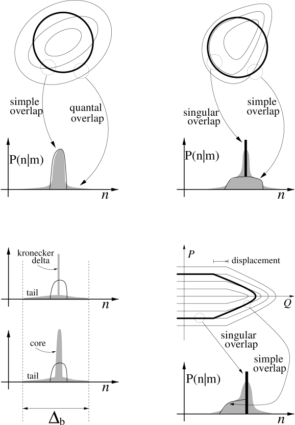
Figure 5: Upper Left: Phase space illustration of the initial and of the instantaneous set of parametric energy surfaces; Plot of the associated $P(n|m)$, where the classical behavior is indicate by the black lines, and the quantum-mechanical behavior is represented by the grey filling. Detailed QCC is assumed. In the quantum-mechanical case classical sharp-cutoffs are being smeared. Upper Right: Illustration of a typical non-generic feature. In the quantum-mechanical case the classical delta-singularity is being smeared. Lower Right: The same non-generic feature manifests itself in the ‘piston’ example. Lower Left: In the perturbative case there is no detailed QCC. The kernel is characterized by a core-tail structure. The tail is limited by the bandwidth of the coupling matrix-elements. If $\delta x$ is sufficiently small the core is just a Kronecker’s delta.

13 Limitations on quantal-classical correspondence (QCC)

The main objects of our discussion are the transition probability kernel $P_{t}(n|m)$ and the parametric kernel $P(n|m)$ which have been introduced in the previous section. We refer now to Equations (41) and (42). In the classical context $\rho_{n,x}(Q,P)$ is defined as the microcanonical distribution that is supported by the energy-surface ${\cal H}(Q,P;x(t))=E_{n}$. The energy $E_{n}$ corresponds to the phase-space volume $n{=}\Omega(E)$. In the QM context $\rho_{n,x}(Q,P)$ is defined as the Wigner-function that represents the energy-eigenstate $|n(x)\rangle$. The phase-space propagator is denoted symbolically by ${\cal U}(t)$. In the classical case it simply re-positions points in phase-space. In the QM case it has a more complicated structure. It is convenient to measure phase-space volume ($n{=}\Omega(E)$) in units of $(2\pi\hbar)^{d}$ where $d$ is the number of degrees of freedom. This way we can obtain a ‘classical approximation’ for the QM kernel, simply by making $n$ and $m$ integer variables. If the ‘classical approximation’ is similar to the QM kernel, then we say that there is detailed QCC. If only the second-moment is similar, then we say that there is restricted QCC. In the present section we are going to discuss the conditions for having detailed QCC, using simple semiclassical considerations.

Wigner function $\rho_{n,x}(Q,P)$, unlike its classical microcanonical analog, has a non-trivial transverse structure. For a curved energy surface the transverse profile looks like Airy function and it is characterized by a width [22]

$$\Delta_{\mbox{\tiny SC}}\ =\ \left(\varepsilon_{\mbox{\tiny cl}}\left(\frac{\hbar}{\tau_{\mbox{\tiny cl}}}\right)^{2}\right)^{1/3}$$ (45)

where $\varepsilon_{\mbox{\tiny cl}}$ is a classical energy scale. For the ‘piston’ example $\varepsilon_{\mbox{\tiny cl}}=E$ is the kinetic energy of the gas particle. In the next paragraph we discuss the conditions for having detailed QCC in the computation of the parametric kernel $P(n|m)$. Then we discuss the further restrictions on QCC, that are associated with the actual kernel $P_{t}(n|m)$.

Given a parametric change $\delta x$ we can define a classical energy scale $\delta E_{\mbox{\tiny cl}}\propto\delta x$ via (31). This parametric energy scale characterizes the transverse distance between the intersecting energy-surfaces $|m(x)\rangle$ and $|n(x{+}\delta x)\rangle$. In the generic case, it should be legitimate to neglect the transverse profile of Wigner function provided $\delta E_{\mbox{\tiny cl}}\gg\Delta_{\mbox{\tiny SC}}$. This condition can be cast into the form $\delta x\gg\delta x_{\mbox{\tiny SC}}$ where

$$\delta x_{\mbox{\tiny SC}}\ =\ \frac{\Delta_{\mbox{\tiny SC}}}{\sqrt{\nu_{\mbox{\tiny E}}^{\mbox{\tiny cl}}/\tau_{\mbox{\tiny cl}}}}\ \propto\ \hbar^{2/3}$$ (46)

Another important parametric scale is defined in a similar fashion: We shall see that it is not legitimate to ignore the transverse profile of Wigner function if $\delta E_{\mbox{\tiny cl}}<\Delta_{b}$. This latter condition can be cast into the form $\delta x\ll\delta x_{\mbox{\tiny prt}}$ where

$$\delta x_{\mbox{\tiny prt}}\ =\ \frac{\Delta_{b}}{\sqrt{\nu_{\mbox{\tiny E}}^{\mbox{\tiny cl}}/\tau_{\mbox{\tiny cl}}}}\ =\ \frac{\hbar}{\sqrt{\nu_{\mbox{\tiny E}}^{\mbox{\tiny cl}}\tau_{\mbox{\tiny cl}}}}$$ (47)

Typically the two parametric scales are well separated ($\delta x_{\mbox{\tiny prt}}\ll\delta x_{\mbox{\tiny SC}}$). If we have $\delta x\ll\delta x_{\mbox{\tiny prt}}$ then the parametric kernel $P(n|m)$ is characterized by a perturbative core-tail structure which is illustrated in Fig.5 and further discussed in the next sections. We do not have a theory for the intermediate parametric regime $\delta x_{\mbox{\tiny prt}}\ll\delta x\ll\delta x_{\mbox{\tiny prt}}$. But for $\delta x\gg\delta x_{\mbox{\tiny SC}}$ we can argue that there is a detailed QCC between the quantal kernel and the classical kernel. Obviously, ‘detailed QCC’ does not mean complete similarity. The classical kernel is typically characterized by various non-Gaussian features, such as sharp cutoffs, delta-singularities and cusps. These features are expected to be smeared in the quantum-mechanical case.

We turn now to discuss the actual transition probability kernel $P_{t}(n|m)$. Here we encounter a new restriction on detailed QCC: The evolving surface ${\cal U}(t)|m\rangle$ becomes more and more convoluted as a function of time. This is because of the mixing behavior that characterizes chaotic dynamics. For $t>t_{\mbox{\tiny scl}}$ the intersections with a given instantaneous energy surface $|n\rangle$ become very dense, and associated quantum-mechanical features can no longer be ignored. The time scale $t_{\mbox{\tiny scl}}$ can be related to the failure of the stationary phase approximation [23].

The breaktime scale $t_{\mbox{\tiny scl}}$ of the semiclassical theory is analogous to the breaktime scale $t_{\mbox{\tiny prt}}$ of perturbation theory, as well as to the breaktime scale $t_{\mbox{\tiny frc}}$ of the classical theory. In order to establish the crossover from ballistic to diffusive energy spreading using QCC considerations we should satisfy the condition $\tau_{\mbox{\tiny cl}}\ll t_{\mbox{\tiny scl}}$. This velocity-independent condition is not very restrictive. On the other hand we should also satisfy the condition $\delta x\gg\delta x_{\mbox{\tiny SC}}$, with $\delta x=V\tau_{\mbox{\tiny cl}}$. The latter condition implies that the applicability of the QCC considerations is restricted to relatively fast velocities. We can define:

$$v_{\mbox{\tiny SC}}\ =\ \mbox{\small scaled velocity}\ =\ \sqrt{D_{\mbox{\tiny E}}\ \tau_{\mbox{\tiny cl}}}\ /\ \Delta_{\mbox{\tiny SC}}$$ (48)

If $v_{\mbox{\tiny SC}}\gg 1$ then the classical approximation is applicable in order to analyze the crossover from ballistic to diffusive energy spreading.

14 The parametric evolution of $P(n|m)$

Detailed QCC between the quantal $P(n|m)$ and the classical $P(n|m)$ is not guaranteed if $\delta x<\delta x_{\mbox{\tiny SC}}$. For sufficiently small parametric change $\delta x$, perturbation theory becomes a useful tool for the analysis of this kernel. A detailed formulation of perturbation theory is postponed to later sections. Here we are going to sketch the main observations. We are going to argue that for small $\delta x$ there is no detailed QCC between the quantal and the classical kernels, but there is still restricted QCC that pertains to the second moment of the distribution. Only for large enough $\delta x$ we get detailed QCC. These observations are easily extended to the case of $P_{t}(n|m)$ in the next section.

For extremely small $\delta x$ the parametric kernel $P(n|m)$ has a standard “first-order” perturbative structure, namely:

$$P(n|m)\ \approx\ \delta_{nm}\ +\ \mbox{Tail}(n{-}m)\ \ \ \ \ \mbox{for $\delta x\ll\delta x_{c}^{\mbox{\tiny qm}}$}$$ (49)

where $\delta x_{c}^{\mbox{\tiny qm}}$ is defined as parametric change that is needed in order to mix neighboring levels. For larger values of $\delta x$ neighbor levels are mixed non-perturbatively and consequently we have a more complicated spreading profile:

$$P(n|m)\ \approx\ \mbox{Core}(n{-}m)\ +\ \mbox{Tail}(n{-}m)\ \ \ \ \ \mbox{for $\delta x\ll\delta x_{\mbox{\tiny prt}}$}$$ (50)

In the perturbative regime ($\delta x\ll\delta x_{\mbox{\tiny prt}}$) the second moment of $P(n|m)$ is generically dominated by the ‘tail’. It turns out that the quantum-mechanical expression for the second-moment is classical look-alike, and consequently restricted QCC is satisfied. The core of the quantal $P(n|m)$ is of non-perturbative nature. The core is the component that is expected to become similar (eventually) to the classical $P(n|m)$. A large perturbation $\delta x\gg\delta x_{\mbox{\tiny prt}}$ makes the core spill over the perturbative tail. If we have also $\delta x\gg\delta x_{\mbox{\tiny SC}}$, then we can rely on detailed QCC in order to estimate $P(n|m)$.

For the piston example we can easily get estimates for the various scales involved. These are expressible in terms of De-Broglie wavelength $\lambda_{\mbox{\tiny E}}=2\pi\hbar/(\mathsf{m}v_{\mbox{\tiny E}})$ where $\mathsf{m}$ and $v_{\mbox{\tiny E}}$ are defined as in Section 10. The displacement which is needed in order to mix neighboring levels, and the displacement which is needed in order to mix core and tail, are respectively:

$$\delta x_{c}^{\mbox{\tiny qm}}\ \ \approx\ \ (\lambda_{\mbox{\tiny E}}^{d{+}1}/\mbox{\small Area})^{\mbox{\tiny 1/2}}\ \ \ll\ \ \lambda_{\mbox{\tiny E}}$$ (51)

$$\delta x_{\mbox{\tiny prt}}\ \ \approx\ \ (\tau_{\mbox{\tiny col}}/{\tau_{\mbox{\tiny cl}}})^{\mbox{\tiny 1/2}}\ \lambda_{\mbox{\tiny E}}\ \ \gg\ \ \lambda_{\mbox{\tiny E}}$$ (52)

We have, in the generic case as well as in the case of the ‘piston’, the hierarchy $\delta x_{c}^{\mbox{\tiny qm}}\ll\delta x_{\mbox{\tiny prt}}\ll\delta x_{\mbox{\tiny SC}}$. Thus there is a ‘gap’ between the perturbative regime ($\delta x\ll\delta x_{\mbox{\tiny prt}}$) and the semiclassical regime ($\delta x\gg\delta x_{\mbox{\tiny SC}}$).

15 The time evolution of $P_{t}(n|m)$

The dynamical evolution of $P_{t}(n|m)$ is related to the associated parametric evolution of $P(n|m)$. We can define a perturbative time scale $t_{\mbox{\tiny prt}}$ which is analogous to $\delta x_{\mbox{\tiny prt}}$. For $t\ll t_{\mbox{\tiny prt}}$ the kernel $P_{t}(n|m)$ is characterized by a core-tail structure that can be analyzed using perturbation theory. In particular we can determine the second moment of the energy distribution, and we can establish restricted QCC. If the second moment for the core-tail structure is proportional to $t^{2}$, we shall say that there is a ballistic-like behavior. If it is proportional to $t$, we shall say that there is a diffusive-like behavior. In both cases the actual energy distribution is not classical-like, and therefore the term ’ballistic’ and ‘diffusive’ should be used with care. We are going now to give a brief overview of the various scenarios in the time evolution of $P_{t}(n|m)$. These are illustrated in Fig.6. In later sections we give a detailed account of the theory.

Figure 6: The various crossovers in the time evolution of $P_{t}(n|m)$. The vertical axis is $x(t)=Vt$. The parametric scales $\delta x_{c}^{\mbox{\tiny qm}}$ and $\delta x_{\mbox{\tiny prt}}$ are indicted by horizontal lines. The horizontal axis is the velocity $V$. It is divided by vertical dashed lines to various velocity regimes. In each velocity regime there is a different dynamical route. The various crossovers are explained in the text and the various symbols are easily associated with having either Gaussian or some non-Gaussian spreading profile. In particular the perturbative spreading profile is either with or without non-trivial core, and its tail is either band-limited or resonance-limited.

For slow velocities such that $\tau_{\mbox{\tiny cl}}\ll t_{\mbox{\tiny prt}}\ll t_{\mbox{\tiny H}}$, there is a crossover from ballistic-like spreading to diffusive-like spreading at $t\sim\tau_{\mbox{\tiny cl}}$. In spite of the lack of detailed QCC there is still restricted QCC as far as this ballistic-diffusive crossover is concerned. The breakdown of perturbation theory before the Heisenberg time ($t_{\mbox{\tiny prt}}\ll t_{\mbox{\tiny H}}$) implies that there is a second crossover at $t\sim t_{\mbox{\tiny prt}}$ from a diffusive-like spreading to a genuine diffusive behavior.

extremely slow velocities are defined by the the inequality $t_{\mbox{\tiny H}}\ll t_{\mbox{\tiny prt}}$. This inequality implies that there are quantum-mechanical recurrences before the expected crossover from diffusive-like spreading to genuine-diffusion. This is the quantum-mechanical adiabatic regime. In the $t\rightarrow\infty$ limit Landau-Zener transitions dominate the energy spreading, and consequently neither detailed nor restricted QCC is a-priori expected [15].

For fast velocities we have $t_{\mbox{\tiny prt}}\ll\tau_{\mbox{\tiny cl}}$. There is a crossover at $t\sim t_{\mbox{\tiny prt}}$ from ballistic-like spreading to a genuine ballistic behavior, and at $t\sim\tau_{\mbox{\tiny cl}}$ there is a second crossover from genuine-ballistic to genuine-diffusive spreading. The description of this classical-type crossover is out-of-reach for perturbation theory, but we can use the semiclassical picture instead. Note that the semiclassical definition of ‘fastness’ and the perturbative definition of ‘slowness’ imply that there is a ‘gap’ between the corresponding regimes. However, the interpolation is smooth, and therefore for simple systems surprises are not expected.

16 Linear response theory

The classical derivation in Section 8 applies also in the quantum-mechanical case provided ${\cal F}(t)$ is treated as an operator. This is known as ‘linear response theory’, and the expression for $D_{\mbox{\tiny E}}$ is essentially the ‘Kubo-Greenwood’ formula. Obviously the restriction $t\ll t_{\mbox{\tiny frc}}$ is replaced by the more restrictive condition $t\ll t_{\mbox{\tiny prt}}$, which will be discussed later. For the purpose of concise presentation, the formula for the energy spreading can be written as follows:

$$\delta E^{2}\ =\ V^{2}\int_{0}^{t}\int_{0}^{t}C_{\mbox{\tiny E}}(t_{2}{-}t_{1})dt_{1}dt_{2}\ =\ V^{2}t\int_{-\infty}^{+\infty}\frac{d\omega}{2\pi}\tilde{C}_{\mbox{\tiny E}}(\omega)\ \tilde{F}_{t}(\omega)$$ (53)

$$\mbox{where}\hskip 56.9055pt\tilde{F}_{t}(\omega)\ =\ t{\cdot}(\mbox{sinc}(\omega t/2))^{2}$$ (54)

The power spectrum of the classical fluctuations looks like white noise. It satisfies $\tilde{C}_{\mbox{\tiny E}}(\omega)\approx\nu_{\mbox{\tiny E}}$ for $|\omega|<1/\tau_{\mbox{\tiny cl}}$ and decays to zero outside of this regime. Thus, still considering the classical case, for $t\ll\tau_{\mbox{\tiny cl}}$ we can make the replacement $\tilde{F}_{t}(\omega)\rightarrow t$, and we obtain the ballistic result $\delta E^{2}=C_{\mbox{\tiny E}}(0){\cdot}(Vt)^{2}$, while for $t\gg\tau_{cl}$ we can make the replacement $\tilde{F}_{t}(\omega)\rightarrow 2\pi\delta(\omega)$, and we get then the diffusive behavior $\delta E^{2}=\nu_{\mbox{\tiny E}}V^{2}t$. Now we turn to the quantum-mechanical case. The power-spectrum of the quantum-mechanical fluctuations is given by the formula

$$\tilde{C}_{\mbox{\tiny E}}(\omega)\ =\ \sum_{n}^{\prime}\left|\left(\frac{\partial{\cal H}}{\partial x}\right)_{nm}\right|^{2}\ 2\pi\delta\left(\omega-\frac{E_{n}{-}E_{m}}{\hbar}\right)$$ (55)

Semiclassical reasoning [24] applied to (55) leads to the immediate conclusion that energy levels are coupled by matrix elements provided $|E_{n}-E_{m}|<\Delta_{b}$ where

$$\Delta_{b}\ =\ \frac{\hbar}{\tau_{\mbox{\tiny cl}}}\ =\ \mbox{band width}$$ (56)

The discrete nature of the power spectrum is of no significance as long as $t\ll t_{\mbox{\tiny H}}$. Therefore we have a crossover from ballistic to diffusive behavior as in the classical case. On the other hand, if $t\gg t_{\mbox{\tiny H}}$ we have $\delta E^{2}\sim\mbox{const}$. This is due to quantum-mechanical recurrences [18]. We shall argue that the latter result is valid only for extremely slow velocities, for which $t_{\mbox{\tiny H}}\ll t_{\mbox{\tiny prt}}$, and provided Landau-Zener transitions are ignored. This is the quantum-mechanical adiabatic regime. For non extremely slow velocities we have $t_{\mbox{\tiny H}}\gg t_{\mbox{\tiny prt}}$, and consequently there is a second crossover at $t=t_{\mbox{\tiny prt}}$ from diffusive-like behavior to genuine diffusion. In the latter case there are no recurrences, and QCC holds also for $t>t_{\mbox{\tiny H}}$.

17 Actual and Parametric Dynamics

The simplicity of linear response theory is lost once we try to formulate a controlled version of it. Therefore it is better to use a more conventional approach and to view the energy spreading as arising from transitions between energy levels. The transition probability kernel and the parametric kernel can be written using standard Dirac notations as follows:

$$P_{t}(n|m)\ =\ |{\mathbf{U}}_{nm}(t)|^{2}\ =\ \left|\langle n(x(t))|{\mathbf{U}}(t)|m(0)\rangle\right|^{2}$$ (57)

$$P(n|m)\ =\ |{\mathbf{T}}_{nm}(x)|^{2}\ =\ \left|\langle n(x)|m(0)\rangle\right|^{2}$$ (58)

The evolution matrix ${\mathbf{U}}_{nm}(t)$ can be obtained by solving the Schroedinger equation

$$\frac{da_{n}}{dt}\ =\ -\frac{i}{\hbar}E_{n}\ a_{n}\ -\frac{i}{\hbar}\sum_{m}{\mathbf{W}}_{nm}(x(t))\ a_{m}$$ (59)

$$\mbox{where}\hskip 56.9055pt{\mathbf{W}}_{nm}\ =\ i\frac{\hbar\dot{x}}{E_{n}{-}E_{m}}\Big{\langle}n\Big{|}\frac{\partial{\cal H}}{\partial x}\Big{|}m\Big{\rangle}$$ (60)

The derivation of (59) follows standard procedure [20]. The transformation matrix ${\mathbf{T}}_{nm}$ can be obtained by considering the same equation with the first term on the right hand side omitted. We shall refer to ${\mathbf{T}}_{nm}(x(t))$ as describing the parametric dynamics (PD), while ${\mathbf{U}}_{nm}(t)$ describes the actual dynamics (AD). For PD the velocity $\dot{x}=V$ plays no role, and it can be scaled out from the above equation. Consequently, for PD, parametric scales and temporal scales are trivially related via the scaling transformation $\delta x=V\tau$. For short times, as long as the energy differences between the participating levels are not yet resolved, the AD coincided with the PD. This is the quantum-mechanical sudden approximation, which we are going to further discuss later on.

         Classical Parameters: $\tau_{\mbox{\tiny cl}}$ = correlation time $D_{\mbox{\tiny E}}$ = $\frac{1}{2}\ \nu_{\mbox{\tiny E}}\ V^{2}$ Quantum-Mechanical Parameters: $\Delta_{b}$ = band width $\Delta$ = level spacing Primary Dimensionless Parameters: $v_{\mbox{\tiny PR}}$ = scaled velocity = $\sqrt{D_{\mbox{\tiny E}}\ \tau_{\mbox{\tiny cl}}}\ /\ \Delta_{b}$ $b$ = scaled band width = ${\Delta_{b}}\ /\ {\Delta}$ Secondary Dimensionless Parameters: $v_{\mbox{\tiny RMT}}$ = $b^{\mbox{\tiny 1/2}}\ v_{\mbox{\tiny PR}}$ = $\tau_{\mbox{\tiny cl}}\ /\ \tau_{c}^{\mbox{\tiny qm}}$ $v_{\mbox{\tiny LZ}}$ = $b^{\mbox{\tiny 3/2}}\ v_{\mbox{\tiny PR}}$ = $t_{\mbox{\tiny H}}\ /\ \tau_{c}^{\mbox{\tiny qm}}$         

Table 1: Generic parameters in the classical and in the quantum-mechanical theories of dissipation. Note that quantum-mechanics requires the specification of two additional parameters. However, for the purpose of QCC considerations only $\Delta_{b}$ is significant. Note that $v_{\mbox{\tiny LZ}}\gg v_{\mbox{\tiny RMT}}\gg v_{\mbox{\tiny PR}}$. In the classical limit all of them $\gg 1$.

The generic parameters that appear in the quantum-mechanical theory are summarized in Table I. The specification of the mean level spacing $\Delta$ is not dynamically significant as long as $t\ll t_{\mbox{\tiny H}}$. Longer times are required in order to resolve individual energy levels. Thus we come to the conclusion that in the time regime $t<t_{\mbox{\tiny H}}$ there is a single generic dimensionless parameter, namely $v_{\mbox{\tiny PR}}$, that controls QCC. We shall see that the quantum mechanical definition of slowness, namely $\tau_{\mbox{\tiny cl}}\ll t_{\mbox{\tiny prt}}$, can be cast into the form $v_{\mbox{\tiny PR}}\ll 1$. On the other hand in the classical limit we have $v_{\mbox{\tiny PR}}\gg v_{\mbox{\tiny SC}}\gg 1$. Thus the dimensionless parameter $v_{\mbox{\tiny PR}}$ marks a border between two regimes where different considerations are required in order to establish QCC.

18 Perturbation theory

We can use Equation (59) as a starting point for a conventional first-order perturbation theory. For short times, such that $P_{t}(m|m)\sim 1$, the transition probability from level $m$ to level $n$ is determined by the coupling strength $|{\mathbf{W}}_{nm}|^{2}$, by the energy difference $(E_{n}{-}E_{m})$ and by the correlation function $F(\tau)$. The latter describes loss of correlation between ${\mathbf{W}}_{nm}(x(0))$ and ${\mathbf{W}}_{nm}(x(t))$. It is defined via

$$\left\langle\ {\mathbf{W}}_{nm}^{\star}(t{+}\tau)\ {\mathbf{W}}_{nm}(t)\ \right\rangle\ =\ \ |W_{nm}|^{2}\ F(\tau)$$ (61)

with the convention $F(0)=1$. It is now quite straightforward [20] to obtain, using first-order perturbation theory, the following result:

$$P_{t}(n|m)\ \approx\ t\tilde{F}_{t}\left(\frac{E_{n}{-}E_{m}}{\hbar}\right)\times\left|\frac{{\mathbf{W}}_{nm}}{\hbar}\right|^{2}\ \ \ \ \ \ \mbox{for $n\neq m$}\ \ \ .$$ (62)

The function $\tilde{F}_{t}(\omega)$ describes the spectral content of the perturbation. For a constant perturbation ($F(\tau)=1$) it is just given by equation (54). For a noisy perturbation $F(\tau)$ is characterized by some finite correlation-time $\tau_{c}$, and therefore the function $\tilde{F}_{t}(\omega)$ is modified as follows:

$$\tilde{F}_{t}(\omega)\ =\ \tilde{F}(\omega)\ \ \ \ \mbox{for $t>\tau_{c}$}$$ (63)

where $\tilde{F}(\omega)$ is the Fourier transform of the correlation function $F(\tau)$. In order to use (62) we should determine how $F(\tau)$ look like, and in particular we should determine what is the correlation-time $\tau_{c}$. We postpone this discussion, and assume that $F(\tau)$ and hence $\tau_{c}$ are known from some calculation. The total transition probability is $p(t)=\sum_{n}^{\prime}P(n|m)$, where the prime indicates omission of the term $n=m$. First order perturbation theory is valid as long as $p(t)\ll 1$. This defines the breaktime $t_{\mbox{\tiny prt}}^{\prime}$ of the perturbative treatment. We use the notation $t_{\mbox{\tiny prt}}^{\prime}$ rather than $t_{\mbox{\tiny prt}}$, since later we are going to define an improved perturbative treatment where $t_{\mbox{\tiny prt}}$ is defined differently.

Using the above first-order perturbative result we can obtain the previously discussed expression (53) for the energy spreading:

$$\delta E^{2}\ =\ \sum_{n}(E_{n}{-}E_{m})^{2}\ P_{t}(n|m)\ =\ V^{2}t\int_{-\infty}^{+\infty}\frac{d\omega}{2\pi}\tilde{C}_{\mbox{\tiny E}}(\omega)\ \tilde{F}_{t}(\omega)$$ (64)

We see that the perturbative result would coincides with the linear-response result only if the coupling matrix-elements could have been treated as constant in time. The above derivation imply that we can trust this formula only for a short time $t<t_{\mbox{\tiny prt}}^{\prime}$. However, later we shall see that it can be trusted for a longer time $t<t_{\mbox{\tiny prt}}$.

It is now possible to formulate the conditions for having restricted QCC. By ‘restricted’ QCC we mean that only $\delta E^{2}$ is being considered. We assume that the result (64) is valid for $t<t_{\mbox{\tiny prt}}$. We also assume that $t_{\mbox{\tiny prt}}$ as well as $F(\tau)$ and hence $\tau_{c}$ are known from some calculation. The following discussion is meaningful if and only if the following Fermi-golden-rule (FGR) condition is satisfied:

$$\mbox{\bf FGR-condition:}\ \ \ \ \mbox{Either}\ \tau_{\mbox{\tiny cl}}\ \mbox{or}\ \tau_{c}\ \ \ \ll\ \ \ t_{\mbox{\tiny prt}}$$ (65)

It is essential to distinguish between two different possible scenarios:

Resonance-limited transitions: $$\tau_{c}\gg\tau_{\mbox{\tiny cl}}$$ (66)

Band-limited transitions: $$\tau_{c}\ll\tau_{\mbox{\tiny cl}}$$ (67)

For resonance-limited transitions, finite $\tau_{c}$ has no consequence as far as $\delta E^{2}$ is concerned: The crossover to diffusive behavior $\delta E^{2}\propto t$ happens at $t\sim\tau_{\mbox{\tiny cl}}$, and this diffusive behavior persists for $t>\tau_{c}$ with the same diffusion coefficient. On the other hand, for band-limited transitions we have at $t\sim\tau_{c}$ a pre-mature crossover from ballistic to diffusive behavior. Consequently the classical result is suppressed by a factor $(\tau_{c}/\tau_{\mbox{\tiny cl}})\ll 1$. This is due to the fact that the transitions between levels are limited not by the resonance width (embodied by $\tilde{F}(\omega)$), but rather by the band-width of the coupling matrix elements (embodied by $\tilde{C}_{\mbox{\tiny E}}(\omega)$).

19 The over-simplified RMT picture

In order to have practical estimates for $t_{\mbox{\tiny prt}}^{\prime}$ and $\tau_{c}$ it is required to study the statistical properties of the matrix ${\mathbf{W}}_{nm}$. This matrix is banded, and its elements satisfy:

$$\left\langle\left|\frac{{\mathbf{W}}_{nm}}{\hbar}\right|^{2}\right\rangle\ \approx\ \left(\frac{1}{\tau_{c}^{\mbox{\tiny qm}}}\right)^{2}\ \frac{1}{(n{-}m)^{2}}\ \ \ \ \ \mbox{for}\ \ |n{-}m|<b/2$$ (68)

The time scale $\tau_{c}^{\mbox{\tiny qm}}$ is related via $\delta x=V\tau$ to the parametric scale

$$\delta x_{c}^{\mbox{\tiny qm}}\ =\ \frac{\Delta}{\sqrt{\langle|({\partial{\cal H}}/{\partial x})_{nm}|^{2}\rangle}}\ \approx\ \sqrt{\frac{2\pi\hbar\Delta}{\nu_{\mbox{\tiny E}}^{\mbox{\tiny cl}}}}$$ (69)

This is the parametric change which is required in order to mix neighboring levels. Given two levels $n$ and $m$ one observes that $\delta x_{c}^{\mbox{\tiny qm}}$ also determines the correlation scale of the matrix-element ${\mathbf{W}}_{nm}(x(t))$. These observations can be summarized as follows:

$$t_{\mbox{\tiny prt}}^{\prime}\ =\ \tau_{c}\ =\ \tau_{c}^{\mbox{\tiny qm}}\ \ \ \ \ \mbox{for standard perturbation theory.}$$ (70)

In the regime $v_{\mbox{\tiny RMT}}\ll 1$ we have $\tau_{c}\gg\tau_{\mbox{\tiny cl}}$. Therefore we have resonance limited transitions and we can relay on (64) in order to establish restricted QCC. On the other hand in the regime $v_{\mbox{\tiny RMT}}\gg 1$ the FGR condition (65) is not satisfied, and the expected crossover at $t=\tau_{\mbox{\tiny cl}}$ is out-of-reach as far as the standard version of perturbation theory is concerned.

In the spirit of random-matrix-theory (RMT) we may think of ${\mathbf{W}}_{nm}(x)$ of Equation (59) as a particular realization which is taken out from some large ensemble of (banded) random matrices. In order to have a well defined mathematical model we should specify the $x$-correlations as well. It looks quite innocent to assume that the only significant correlations are those expressed in Eq.(61). In other words, let us assume, following [16], that cross correlations between matrix elements can be ignored. One finds then that (64) should hold for classically long times. This claim can be summarized as follows:

$$t_{\mbox{\tiny prt}}=t_{\mbox{\tiny frc}}\ \ \ \ \ \ \mbox{and}\ \ \ \ \ \ \tau_{c}=\tau_{c}^{\mbox{\tiny qm}}\ \ \ \ \ \ \mbox{for the over-simplified RMT picture.}$$ (71)

If the over-simplified RMT assumption were true it would imply that in the $v_{\mbox{\tiny RMT}}\gg 1$ regime the transitions would be band-limited and consequently classical diffusion would be suppressed by a factor $(1/v_{\mbox{\tiny RMT}})\ll 1$. Note that in the semiclassical limit we have indeed $v_{\mbox{\tiny RMT}}\gg 1$. Therefore, it is implied that the classical limit would not coincide with the classical result. Obviously, we expect this conclusion to be wrong, and indeed we shall demonstrate that cross correlations between matrix elements cannot be ignored. This will be done by transforming the Schroedinger equation to a more appropriate basis.

20 The perturbative core-tail spreading profile

The standard version of perturbation theory is valid for an extremely short time. See (70). In order to formulate an improved version of perturbation theory it is essential to understand the perturbative structure of $P_{t}(n|m)$. Once $t>\tau_{c}^{\mbox{\tiny qm}}$ neighboring levels are mixed and consequently the probability kernel acquires a non-trivial core-tail structure which is illustrated in Fig.7. The ‘improved’ version of perturbation theory should be applicable as long as the core-tail structure is maintained.

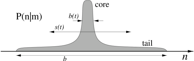
Figure 7: Schematic illustration of a generic core-tail spreading profile. The core-width $b(t)$ is defined by the participation-ratio. The second-moment should satisfy $b(t)\ll s(t)\ll b$, where $b$ is that bandwidth. In case of $P_{t}(n|m)$ the tail becomes (for $t>\tau_{\mbox{\tiny cl}}$) resonance-limited rather than band-limited. In the resonance-limited case the bandwidth $b$ in the above figure should be replaced by $(\hbar/t)/\Delta$, and accordingly the requirement is $b(t)\ll s(t)\ll(\hbar/t)/\Delta$.

Now we shall characterize the main features of a generic core-tail spreading profile. The expression for the probability kernel $P_{t}(n|m)$ can be written schematically as follows:

$$P_{t}(n|m)\ \approx\ \mbox{Core}(n{-}m)\ +\ \mbox{Tail}(n{-}m)\ \ \ \ \ \mbox{for $t<t_{\mbox{\tiny prt}}$}$$ (72)

The kernel is characterized by two scales:

$$b(t)\ =\ \mbox{\small core width}\ = \ \left(\sum_{n}(P_{t}(n|m))^{2}\right)^{-1}$$ (73)

$$s(t)\ =\ \mbox{\small spreading}\ = \ \left(\sum_{n}(n{-}m)^{2}\ P_{t}(n|m)\right)^{-1/2}$$ (74)

such that $b(t)\ll s(t)\ll b$. For $t\ll\tau_{c}^{\mbox{\tiny qm}}$ we have a trivial core with $b(t)\approx 1$, whereas for $t\gg\tau_{c}^{\mbox{\tiny qm}}$ we have a non-trivial core with $b(t)\gg 1$. The matrix elements satisfy $\langle|{\mathbf{W}}_{nm}|^{2}\rangle\ \propto\ 1/(n{-}m)^{2}$. We shall see (see (78)) that in the ‘band-limited tail’ case we have $P_{t}(n|m)\sim\mbox{const}/(n{-}m)^{2}$ up to the cutoff $b$, while for the ‘resonance-limited tail’ case we have $P_{t}(n|m)\sim\mbox{const}/(n{-}m)^{2}$ up to the cutoff $(\hbar/t)/\Delta$. One should realize that the power-law behavior of the tail is ‘fast’ enough in order to guarantee that $b(t)$ is independent of the tail’s cutoff. The cutoff does not have any effect on the evolving core. On the other hand, the second moment $s(t)$, unlike $b(t)$, is predominantly determined by the tail’s cutoff, and it is independent of the core structure.

21 An improved perturbation theory

In order to extend perturbation theory beyond $\tau_{c}^{\mbox{\tiny qm}}$ it is essential to eliminate the non-perturbative transitions within the core. This can be done by making a transformation to an appropriate basis as follows:

$$a_{n}(t)\ = \ \sum_{m}\tilde{\mathbf{T}}_{nm}\ c_{m}(t)$$ (75)

$$\tilde{\mathbf{T}}_{nm} = {\mathbf{T}}_{nm}\ \ \ \mbox{if $|n{-}m|<b^{\prime}/2$, else zero.}$$ (76)

The amplitudes $c_{n}(t)$ satisfy the same Schroedinger equation as the $a_{n}(t)$, with a transformed matrix $\tilde{\mathbf{W}}$. The general expression for $\tilde{\mathbf{W}}$ is quite complicated, but we are interested only in the core-to-tail transitions for which

$$(\tilde{\mathbf{W}})_{nm}=(\tilde{\mathbf{T}}^{\dagger}\mathbf{W}\tilde{\mathbf{T}})_{nm}\ \ \ \mbox{for $|n{-}m|>b^{\prime}$}$$ (77)

(no approximation is involved). Once this transformation is performed the ‘new’ Schroedinger equation is characterized by a new correlation time $\tau_{c}$ and by a new perturbative time $t_{\mbox{\tiny prt}}^{\prime}$. Both $\tau_{c}$ and $t_{\mbox{\tiny prt}}^{\prime}$ depend on the free parameter $b^{\prime}$. Our choice of the course-graining parameter $b^{\prime}$ is not completely arbitrary. The restrictions are:
 
$\hskip 5.69054pt\bullet\ \$ Unitarity is approximately preserved:          $b(t)\ \ll\ b^{\prime}$.
$\hskip 5.69054pt\bullet\ \$ Core-to-Tail transitions are preserved:          $b^{\prime}\ \ll\ b$.
$\hskip 5.69054pt\bullet\ \$ Long effective correlation time is attained:     $\tau_{\mbox{\tiny cl}}\ \ll\ \tau_{c}$
 
The feasibility of the last requirement deserves further discussion. One should realize that for $b^{\prime}=b$ we are actaully transforming the Schrodinger equation to an $x$-independent basis. Therefore the transformed matrix $\tilde{\mathbf{T}}^{\dagger}\mathbf{W}\tilde{\mathbf{T}}$ becomes correlated on a time scale $\tau_{c}^{\mbox{\tiny cl}}$, which has been discussed in Section 5. As we change $b^{\prime}$ from $b$ to smaller values, we expect $\tau_{c}$ to become smaller. By continuity, we expect no difficulty in satisftying the conditions $b^{\prime}\ll b$ and $\tau_{c}\gg\tau_{\mbox{\tiny cl}}$ simultaneously.

The usefullness of the above transformation stems from the fact that due to the elimination of non-perturbative transitions within the core, $t_{\mbox{\tiny prt}}^{\prime}$ becomes much longer than $\tau_{c}^{\mbox{\tiny qm}}$. At the same time the information which is required in order to determine the second moment $s(t)$ is not lost. We have $|\tilde{\mathbf{W}}_{nm}|\approx|{\mathbf{W}}_{nm}|$ for core-to-tail transitions, and a practical approximation for the ‘renormalized’ spreading profile would be

$$P_{t}(n|m)\ \sim\ \delta_{nm}\ +\ t\tilde{F}_{t}\left(\frac{E_{n}{-}E_{m}}{\hbar}\right)\times\left(\frac{1}{\tau_{c}^{\mbox{\tiny qm}}}\right)^{2}\ \frac{1}{(b^{\prime})^{2}+(n{-}m)^{2}}$$ (78)

The behavior for $|n{-}m|\leq b^{\prime}$ is an artifact of the transformation and contains false information. However, for the calculation of the second moment only the tail is significant. The tail is not affected by our transformation and therefore we obtain the same result (64) for $\delta E^{2}$ with one important modification: a different effective value for $\tau_{c}$. Moreover, since $b^{\prime}$ is chosen such that $\tau_{c}\gg\tau_{\mbox{\tiny cl}}$, it follows that the transitions are resonant-limited and consequently restricted QCC is established also in the domain $v_{\mbox{\tiny RMT}}>1$.

The validity of the above QCC considerations is conditioned by having $\tau_{\mbox{\tiny cl}}\ll t_{\mbox{\tiny prt}}^{\prime}$. Breakdown of the present version of perturbation theory happens once the total transition probability in (78) becomes non-negligible (of order 1). Thus

$$t_{\mbox{\tiny prt}}^{\prime}\ =\ (b^{\prime})^{\mbox{\tiny 1/2}}\times\tau_{c}^{\mbox{\tiny qm}}\ \ \ \ \ \mbox{for the improved perturbation theory.}$$ (79)

It is easily verified that the latter condition $\tau_{\mbox{\tiny cl}}\ll t_{\mbox{\tiny prt}}^{\prime}$ cannot be satisfied if $v_{\mbox{\tiny PR}}>1$. This is not just a technical limitation of our perturbation theory, but reflects a real difference between two distinct routes towards QCC. This point is further illuminated in the next sections.

22 Consequences of the improved perturbative treatment

Our perturbation theory is capable of giving information about the tail, and hence about the second moment. Given $t$, one wonders how much $b^{\prime}$ can be ‘pushed down’ without violating the validity conditions of our procedure. It is quite clear that $b^{\prime}\gg b(t)$ is a necessary condition for not having a breakdown of perturbation theory. If we assume that the energy-spreading-profile is characterized just by the single parameter $b(t)$, then the condition $b^{\prime}\gg b(t)$ should be equivalent to $t\ll t_{\mbox{\tiny prt}}^{\prime}$. Hence the following estimate is suggested:

$$b(t)\ =\ (t/\tau_{c}^{\mbox{\tiny qm}})^{2}$$ (80)

If we want to have a better idea about the core structure we should apply, in any special example, specific (non-perturbative) considerations. For example, in case of the piston example we can use semiclassical considerations in order to argue [21] that the core has a Lorentzian shape whose width is $\hbar/\tau_{\mbox{\tiny col}}$. This structure is exposed provided $\hbar/\tau_{\mbox{\tiny col}}\ll b(t)$, leading to the condition $\delta x\gg\lambda_{\mbox{\tiny E}}$. Else we have a structure-less core whose width is characterized by the single parameter $b(t)$.

We turn now to determine the $\delta x_{\mbox{\tiny prt}}$ of the parametric dynamics (PD), and then the $t_{\mbox{\tiny prt}}$ of the actual dynamics (AD). Recall that PD is obtained formally by ignoring the differences $(E_{n}{-}E_{m})$, which implies that we can make in (78) the replacement $\tilde{F}_{t}\mapsto t$. Thus the tail of $P(n|m)$ is band-limited and consequently the second moment is

$$s(t)^{2}\ =\ b\times(1/\tau_{c}^{\mbox{\tiny qm}})^{2}\ t^{2}\ \ \ \mbox{[band-limited tail]}$$ (81)

in agreement with the classical ballistic result. Our procedure for analyzing the core-tail structure of $P(n|m)$ is meaningful as long as we have $b(t)\ll s(t)\ll b$. This defines an upper time limitation $t_{\mbox{\tiny prt}}=\delta x_{\mbox{\tiny prt}}/V$, where

$$\delta x_{\mbox{\tiny prt}}\ =\ b^{\mbox{\tiny 1/2}}\ \delta x_{c}^{\mbox{\tiny qm}}\ =\ \frac{\hbar}{\sqrt{\nu_{\mbox{\tiny E}}^{\mbox{\tiny cl}}\tau_{\mbox{\tiny cl}}}}$$ (82)

At $t=t_{\mbox{\tiny prt}}$ we have $b(t)\sim s(t)\sim b$, and we expect a crossover from a ballistic-like spreading to a genuine ballistic spreading.

The AD departs from the PD once the energy scale $\Delta_{b}$ is resolved. This happens when $t\sim\tau_{\mbox{\tiny cl}}$. The perturbative approach is applicable for the analysis of the crossover at $t\sim\tau_{\mbox{\tiny cl}}$ provided $V\tau_{\mbox{\tiny cl}}\ll\delta x_{\mbox{\tiny prt}}$. This is precisely the condition $v_{\mbox{\tiny PR}}\ll 1$. For $t\gg\tau_{\mbox{\tiny cl}}$ the tail becomes resonance limited ($|n{-}m|<(\hbar/t)/\Delta$) rather than band limited ($|n{-}m|<b$) and we obtain:

$$s(t)^{2}\ =\ (1/\tau_{c}^{\mbox{\tiny qm}})^{2}\ t_{\mbox{\tiny H}}\ t\ \ \ \mbox{[resonance-limited tail]}$$ (83)

in agreement with the classical diffusive result. Our procedure for analyzing the core-tail structure of $P_{t}(n|m)$ is meaningful as long as we have $b(t)\ll s(t)\ll b$. This defines a modified upper time limitation

$$t_{\mbox{\tiny prt}}\ =\ (\tau_{c}^{\mbox{\tiny qm}})^{\mbox{\tiny 2/3}}\ t_{\mbox{\tiny H}}^{\mbox{\tiny 1/3}}\ =\ \left(\frac{\hbar^{2}}{\nu_{\mbox{\tiny E}}V^{2}}\right)^{1/3}\ \ \ \ \ \mbox{[applies to $v_{\mbox{\tiny PR}}\ll 1$]}$$ (84)

At $t=t_{\mbox{\tiny prt}}$ we have $b(t)\sim s(t)\ll b$, and we expect a crossover from a diffusive-like spreading to a genuine diffusive spreading.

23 The quantum mechanical sudden approximation

         Perturbative route ($v_{\mbox{\tiny PR}}\ll 1$): $t_{\mbox{\tiny sdn}}=\tau_{\mbox{\tiny cl}}\ll t_{\mbox{\tiny prt}}$ At   $t=\tau_{\mbox{\tiny cl}}$ $b(t)\ll s(t)\ll b\sim(\hbar/t)/\Delta$ At   $t=t_{\mbox{\tiny prt}}$ $b(t)\sim s(t)\sim(\hbar/t)/\Delta\ll b$ Non-perturbative route ($v_{\mbox{\tiny PR}}\gg 1$): $t_{\mbox{\tiny prt}}\ll t_{\mbox{\tiny sdn}}\ll\tau_{\mbox{\tiny cl}}$ At   $t=t_{\mbox{\tiny prt}}$ $b(t)\sim s(t)\sim b\ll(\hbar/t)/\Delta$ At   $t=t_{\mbox{\tiny sdn}}$ $b\ll s(t)\sim(\hbar/t)/\Delta$ At   $t=\tau_{\mbox{\tiny cl}}$ $b\sim(\hbar/t)/\Delta\ll s(t)$         

Table 2: Various time scales in the route to stochastic behavior.

It is now appropriate to discuss the quantum mechanical sudden approximation. For the perturbative scenario ($v_{{}_{\mbox{\tiny PR}}}\ll 1$) we have already mentioned that the AD departs from the PD at $t_{\mbox{\tiny sdn}}=\tau_{\mbox{\tiny cl}}$, which is the time to resolve the energy scale $\Delta_{b}$. In case of the non-perturbative scenario ($v_{{}_{\mbox{\tiny PR}}}\gg 1$) there is an earlier breakdown of the quantum mechanical sudden approximation. This is because we have $\tau_{\mbox{\tiny cl}}\gg t_{\mbox{\tiny prt}}$ and consequently at $t=\tau_{\mbox{\tiny cl}}$ we already have $s(t)\gg b$. Therefore $t_{\mbox{\tiny sdn}}$ should be defined as the time to resolve the energy scale which is associated with $s(t)$. It leads to

$$t_{\mbox{\tiny sdn}}\ =\ b^{\mbox{\tiny 1/4}}(\tau_{c}^{\mbox{\tiny qm}}\tau_{\mbox{\tiny cl}})^{\mbox{\tiny 1/2}}\ =\ \left(\frac{\hbar^{2}\tau_{\mbox{\tiny cl}}}{\nu_{\mbox{\tiny E}}V^{2}}\right)^{1/4}\hskip 28.45274pt\mbox{for $v_{\mbox{\tiny PR}}\gg 1$}$$ (85)

The various time scales are summarized in Table II. The non-perturbative crossover from genuine-ballistic to genuine-diffusive behavior in not trivial. If $v_{{}_{\mbox{\tiny SC}}}\gg 1$ we can relay on semiclassical considerations in order to establish the existence of this crossover. More generally, for $v_{{}_{\mbox{\tiny PR}}}\gg 1$, we would like to have (but we do not have yet) an appropriate effective RMT model. This effective RMT model should support genuine-ballistic motion, and to be further characterized by an elastic scattering time $\tau_{\mbox{\tiny cl}}$.

24 The quantum mechanical adiabatic approximation

The previous analysis has emphasized the role of core-to-tail transitions in energy spreading. Our assumption was that these transitions are not suppressed by recurrences. This is not true in the quantum-mechanical adiabatic regime ($v_{\mbox{\tiny LZ}}\ll 1$). Following [15] it is argued that energy spreading in the latter regime is dominated (eventually) by Landau-Zener transitions between near-neighbor levels. One obtains

$$D_{\mbox{\tiny E}}^{\mbox{\tiny LZ}}\ \approx\ \left(\frac{1}{v_{\mbox{\tiny LZ}}}\right)^{1{-}(\beta/2)}D_{\mbox{\tiny E}}^{\mbox{\tiny cl}}\hskip 56.9055pt\mbox{for \ $v_{\mbox{\tiny LZ}}\ll 1$}$$ (86)

where $D_{\mbox{\tiny E}}^{\mbox{\tiny cl}}$ is the classical result. The non-trivial nature of Landau-Zener transitions and the statistics of the avoided-crossings is taken into account. One should use $\beta=2$ for the Gaussian unitary ensemble (GUE) and $\beta=1$ for the Gaussian orthogonal ensemble (GOE).

25 Classical Brownian motion

It is possible to argue that the reduced motion of the particle (‘piston’ if the motion is constrained to one dimension) obeys the following Langevin equation:

$$m\ddot{{\mathbf{x}}}+\eta\dot{{\mathbf{x}}}={\cal F}$$ (87)

where $\eta=\mu$ is the friction coefficient. The stochastic force is redefined ${\cal F}:={\cal F}{-}\langle{\cal F}\rangle$, such that it is zero on the average. Its second moment should satisfy

$$\langle{\cal F}(t){\cal F}(t^{\prime})\rangle_{\mbox{\tiny at $x$}}\ =\ \phi(t{-}t^{\prime})$$ (88)

where $\phi(t{-}t^{\prime})=C(t{-}t^{\prime})$. Usually, it is further assumed that higher moments are determined by Gaussian statistics. The correlation time is denoted as before by $\tau_{\mbox{\tiny cl}}$. It is better to view the stochastic force as arising from a stochastic potential

$${\cal F}(t)\ \ =\ \ {\cal F}(t,{\mathbf{x}}(t)) \ =\ -\nabla{\cal U}({\mathbf{x}},t)$$ (89)

$$\langle{\cal U}({\mathbf{x}}^{\prime\prime},t^{\prime\prime}){\cal U}({\mathbf{x}}^{\prime},t^{\prime})\rangle \ =\ \phi(t^{\prime\prime}{-}t^{\prime})\cdot w({\mathbf{x}}^{\prime\prime}{-}{\mathbf{x}}^{\prime})$$ (90)

The spatial correlations of the stochastic potential are assumed to be characterized by a spatial scale $\ell$. The natural tendency is to identify $\ell$ with $\delta x_{c}^{\mbox{\tiny cl}}$, but this point deserves further non-trivial discussion. The normalization convention $w^{\prime\prime}(0)=-1$ is used, and therefore there is consistency of (90) with (88).

26 The DLD Hamiltonian

Formally, the Langevin equation (87) with (90) is an exact description of the reduced dynamics that is generated by the DLD Hamiltonian:

$${\cal H}\ =\ \frac{{\mathbf{p}}^{2}}{2m}\ +\ \sum_{\alpha}c_{\alpha}Q_{\alpha}u({\mathbf{x}}{-}{\mathbf{x}}_{\alpha})\ +\ \sum_{\alpha}\left(\frac{P_{\alpha}^{2}}{2m_{\alpha}}+\frac{1}{2}m\omega_{\alpha}^{2}Q_{\alpha}^{2}\right)$$ (91)

where ${\mathbf{x}}_{\alpha}$ is the location of the $\alpha$ oscillator, $u({\mathbf{x}}-{\mathbf{x}}_{\alpha})$ describes the interaction between the particle and the $\alpha$ oscillator, and $c_{\alpha}$ are coupling constants. It is assumed that the function $u({\mathbf{r}})$ depends only on $|{\mathbf{r}}|$. The range of the interaction is $\ell$. The oscillators are distributed uniformly all over space. Locally, the distribution of their frequencies is ohmic. Namely,

$$\frac{\pi}{2}\sum_{\alpha}\frac{c^{2}_{\alpha}}{m_{\alpha}\omega_{\alpha}}\delta(\omega-\omega_{\alpha})\ \delta({\mathbf{x}}-{\mathbf{x}}_{\alpha})\ =\ \eta\omega\ \ \ \ \mbox{for $\omega<1/\tau_{\mbox{\tiny cl}}$}\ \ \ \ .$$ (92)

This distribution is uniquely determined by the requirement $\phi(\tau)=C(\tau)$. The spatial correlations are determined via

$$w({\mathbf{r}})=\int_{-\infty}^{\infty}u({\mathbf{r}}{-}{\mathbf{x}}^{\prime})u({\mathbf{x}}^{\prime})dx^{\prime}$$ (93)

For example, we may consider a Gaussian $u({\mathbf{r}})$ for which

$$w({\mathbf{r}})\ =\ \ell^{2}\exp\left(-\frac{1}{2}\left(\frac{{\mathbf{r}}}{\ell}\right)^{2}\right)$$ (94)

Certain generalizations of this assumption has been considered in [9], but are of no interest here. In the formal limit $\ell\rightarrow\infty$ the DLD model reduces to the well known ZCL model. The ZCL model is defined by the interaction term $x\cdot\sum c_{\alpha}Q_{\alpha}$.

    

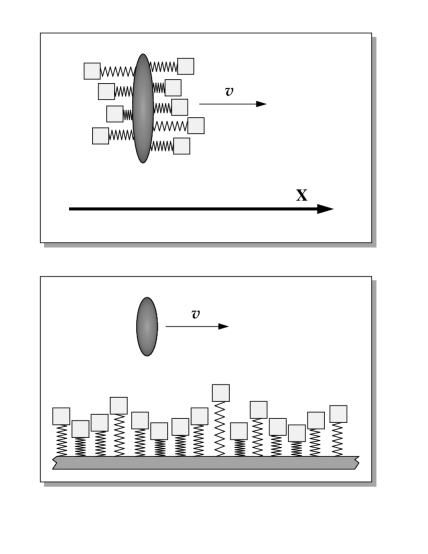
Figure 8: Illustration of the ZCL model (left upper drawing), versus the DLD model (left lower drawing). The instantaneous potential that is experienced by the particle is either linear (right upper drawing), or of disordered nature (right lower drawing) correspondingly. If the fluctuations are uncorrelated in time (WNA), then the two models are classically equivalent. There is no such equivalence in the quantum-mechanical case.

27 The white noise approximation (WNA)

One wonders whether the noise in Langevin equation can be treated as white noise, meaning that $\tau_{\mbox{\tiny cl}}$ is irrelevant and we can set $\tau_{\mbox{\tiny cl}}\sim 0$ in any significant result. The following condition defines the classical notion of white noise:

$$\mbox{Generic Brownian Motion}\ \ \ \ \Leftrightarrow\ \ \ \ \frac{v}{\ell}\ll\frac{1}{\tau_{\mbox{\tiny cl}}}$$ (95)

If the condition is not satisfied, then $\tau_{\mbox{\tiny cl}}$ is larger than $\ell/v$, and the particle performs a stochastic motion that depends crucially on the ‘topography’ of the stochastic potential. Note that upon the identification of $\ell$ with $\delta x_{c}^{\mbox{\tiny cl}}$ the condition above becomes equivalent to the trivial requirement of classical slowness (Sec.5).

In the quantum mechanical analysis it is found that $\phi(\tau)$ is further characterized by a correlation time $\hbar/(k_{\mbox{\tiny B}}T)$. Thus, the following additional requirement should be met if we wish to apply a white noise approximation.

$$\mbox{High Temperatures}\ \ \ \ \Leftrightarrow\ \ \ \ \frac{v}{\ell}\ll\frac{k_{\mbox{\tiny B}}T}{\hbar}$$ (96)

Note that the smallest meaningful velocity is the thermal velocity, and therefore the above condition cannot be satisfied unless the thermal wavelength $\lambda_{\mbox{\tiny T}}=\hbar/(mk_{\mbox{\tiny B}}T)$ is much smaller than $\ell$. From now on we assume that both classically and quantum mechanically we can use the white noise approximation. Thus we can use the formal substitution $\phi(\tau)=\nu\delta(\tau)$.

28 Consequences of the WNA

In the general case, (88) is less informative than (90). However, in case of a classical particle that experiences white noise, the additional information is not required at all! Classically, the spatial correlations, and hence $\ell$, are of no importance. This is because at each moment a classical particle samples one definite point in space. The particle ‘does not care’ about the force elsewhere. In the quantum mechanical case the latter observation is wrong. A quantum mechanical particle samples each moment a finite region in space and therefore spatial correlations of the effective stochastic potential become important, even if the noise is white.

Both classically and quantum mechanically the reduced dynamics that is generated by the DLD model can be obtained analytically and cast into the form

$$\rho_{t}(R,P)\ =\ \int\int dR_{0}dP_{0}\ {\cal K}(R,P|R_{0},P_{0})\rho_{t=0}(R_{0},P_{0})$$ (97)

where $\rho_{t}(R,P)$ represent either the classical-state or the quantum-mechanical-state of the particle. In the latter case it is a Wigner function. It is a consequence of the WNA that the propagator has a Markovian property. Namely, it can be written as the composition of smaller ‘time steps’. Consequently $\rho_{t}(R,P)$ satisfies a master equation of the type

$$\frac{\partial\rho}{\partial t}\ =\ {\cal L}\rho$$ (98)

The classical version of this equation is known as the Fokker-Planck equation. We shall discuss shortly its quantum-mechanical version.

29 The reduced propagator

The reduced propagator of the DLD model can be obtained [8] classically as well as quantum mechanically using a path integral technique. In the quantum mechanical case it is known as the FV-formalism. The classical version of FV formalism can be regarded as a formal solution of Langevin equation. It can be obtained without going via the DLD Hamiltonian, but then one should assume Gaussian statistics.

In the absence of coupling to the environment, the free-motion propagator of Wigner function is the same both classically and quantum mechanically:

$${\cal K}(R,P|R_{0},P_{0})\ =\ {\cal K}_{\mbox{\tiny free}}^{(cl)}\ =\ 2\pi\delta(P{-}P_{0})\ \delta((R{-}R_{0})-\mbox{$\frac{P}{m}$}t)$$ (99)

Taking the environment into account, one obtains, in the classical case,

$${\cal K}(R,P|R_{0},P_{0})\ =\ {\cal K}_{\mbox{\tiny damped}}^{(cl)}\ =\ \mbox{Gaussian}$$ (100)

This result is, as a-priori expected, independent of $\ell$. The average velocity of of the particle goes to zero on a time scale $\tau_{\eta}=(\eta/m)^{-1}$, while the spreading of the Gaussian is

$$\delta p^{2}\ = \ \nu t\ \ \ t\ll\tau_{\eta}$$ for (101)

$$\delta x^{2}\ = \ (1/(3m^{2}))\nu t^{3}\ \ \ \ \ \ \ \ t\ll\tau_{\eta}$$ for (102)

$$\delta p^{2}\ = \ mk_{\mbox{\tiny B}}T\ \ \ t\gg\tau_{\eta}$$ for (103)

$$\delta x^{2}\ = \ (\nu/\eta^{2})t\ \ \ t\gg\tau_{\eta}$$ for (104)

The above result holds also in the quantum mechanical case provided we take the limit $\ell\rightarrow\infty$. No genuine quantum-mechanical effects are found if the ZCL model is used to describe Brownian motion! Recall again that we are considering here the high-temperature case where the WNA applies. Now we want to discuss the finite $\ell$ case. Here one obtains [8, 9] the following expression:

$${\cal K}\ =\ W_{\hbar/\ell}\star{\cal K}_{\mbox{\tiny damped}}^{(cl)}\ +\ \mbox{e}^{-\frac{2\eta k_{B}T\ell^{2}}{\hbar^{2}}t}(1{-}W_{\hbar/\ell}\star)\ {\cal K}_{\mbox{\tiny free}}^{(cl)}$$ (105)

As suspected, unlike in the classical case, the quantum mechanical result depends on $\ell$ in an essential way. $W(R{-}R^{\prime},P{-}P^{\prime})$ is a smooth Gaussian-like kernel that has unit-normalization. Its spread in phase space is characterized by the momentum scale $\hbar/\ell$, and by an associated spatial scale. The symbol $\star$ stands for convolution. Thus, the classical propagator is smeared on a phase-space scale that correspond to $\Delta p=\hbar/\ell$ and there is an additional un-scattered component that decay exponentially and eventually disappears. The structure of the propagator is illustrated in Fig.9. The significance of this structure will be discussed shortly.

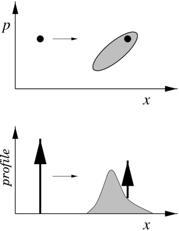
Figure 9: Upper plot: Phase space illustration for the structure of the DLD propagator. Lower plot: The projected phase-space density. Note the existence of an un-scattered component. Such component is absent in the ZCL limit as well as in the classical analysis.

30 Master equation

To write down an explicit expression for the propagator is not very useful. Rather, it is more illuminating to write an equivalent Master equation. This is possible since at high temperatures the propagator possess a Markovian property. The final result [9] is

$$\frac{\partial\rho}{\partial t}\ =\ \left[\ -\ \partial_{R}\ \frac{1}{m}P\ +\ \partial_{P}\ \frac{\eta}{m}G_{F}\star P\ +\ \nu G_{N}\star\right]\ \rho$$ (106)

$$G_{F}\ \equiv\ \ \ \ \ {\cal FT}\left(\frac{w^{\prime}(r)}{r}\right)\ =\ \frac{1}{\hbar/\ell}\hat{G}_{F}\left(\frac{P{-}P^{\prime}}{\hbar/\ell}\right)$$

$$G_{N}\ \equiv\ \frac{1}{\hbar^{2}}{\cal FT}\left(w(r){-}w(0)\right)\ =\ \left(\frac{\ell}{\hbar}\right)^{2}\left[\frac{1}{\hbar/\ell}\hat{G}_{N}\left(\frac{P{-}P^{\prime}}{\hbar/\ell}\right)-\delta(P{-}P^{\prime})\right]$$

For convenience the friction kernel $G_{F}$ and the noise kernel $G_{N}$ are expressed in term of smooth Gaussian-like scaling functions $\hat{G}_{F}$ and $\hat{G}_{N}$ that are properly normalized to unity. The notation ${\cal FT}$ stands for Fourier transform.

If Wigner function does not possess fine details on the momentum scale $\hbar/\ell$, then the convolution with $G_{F}$ can be replaced by multiplication with $1$, and the convolution with $G_{N}$ can be replaced by ${\partial^{2}}/{\partial P^{2}}$. These replacements are formally legitimate both in the classical limit $\hbar\rightarrow 0$, and in the ZCL limit $\ell\rightarrow\infty$. One obtains then the classical Fokker Planck equation

$$\frac{\partial\rho}{\partial t}\ =\ \left[\ -\ \partial_{R}\ \frac{1}{m}P\ +\ \partial_{P}\ \frac{\eta}{m}P\ +\ \nu\frac{\partial^{2}}{\partial P^{2}}\right]\ \rho$$ (107)

The Fokker Planck equation is just a continuity equation with an added noise term that reflects the effect of the stochastic force. The Fokker Planck equation is equivalent to solving Langevin equation as well as to the Gaussian propagator (100).

31 Brownian motion and dephasing

Wigner function may have some modulation on a fine scale due to an interference effect. The standard text-book example of a two slit experiment is analyzed in [9]. In case of the ZCL model ($\ell=\infty$), the propagator is the same as the classical one, and therefore we may adopt a simple Langevin picture in order to analyze the dephasing process. Alternatively, we may regard the dephasing process as arising from Gaussian smearing of the interference pattern by the propagator. In case of the DLD model (finite $\ell$) we should distinguish between two possible mechanisms for dephasing:

• Scattering (Perturbative) Mechanism.

• Spreading (Non-Perturbative) Mechanism.

Actually, it is better to regard them as mechanisms to maintain coherence. The first mechanism to maintain coherence is simply not to be scattered by the environment. The second mechanism to maintain coherence is not to be smeared by the propagator. The first mechanism is absent in case of the ZCL model.

Let us discuss how coherence is lost due to the scattering mechanism. The discussion is relevant if Wigner function contains a modulation on a momentum scale much finer than $\hbar/\ell$, else $\ell$ becomes non-relevant and we can take it to be infinite. One should observe that such modulation is not affected by the friction, but its intensity decays exponentially in time. This is based on inspection of either the propagator (105), or the equivalent Master equation (106). In the latter case note that the convolution with $G_{N}$ can be replaced by multiplication with $-(\ell/\hbar)^{2}$. The decay rate is

$$\frac{1}{\tau_{\varphi}}\ =\ \frac{2\eta k_{B}T\ell^{2}}{\hbar^{2}}\ \ \ \ \ \ \ \ \ \mbox{assuming WNA}$$ (108)

This is the universal result for the dephasing rate due to the ‘scattering mechanism’. It is universal since it does not depend on details of the quantum-mechanical state involved. However, the validity of this result is restricted to the high temperature regime, where the WNA can be applied. Extensions of this result, as well as discussion of dephasing at low temperatures can be found in [9, 11].

32 The open question

The effective-bath approach suggests that there is a universal description of quantal Brownian motion. If indeed the effective-bath approach is universally applicable, it is implied that

$$\mbox{chaos}\hskip 28.45274pt\Longleftrightarrow\hskip 28.45274pt\mbox{dynamical disorder}$$ (109)

meaning that the motion under the influence of chaotic environment is effectively the same as the motion under the influence of dynamical disordered environment.

At this stage the conditions for the validity of (109) are yet unclear. It is interesting however to emphasize the practical implications of such claim. The starting point should be a specification of the effective correlation scale $\ell$. For the ‘piston’ example the most obvious guess is

$$\ell\ =\ \left\{\matrix{\delta x_{c}^{\mbox{\tiny cl}}&\ \ \ \mbox{if}\gg\lambda_{\mbox{\tiny E}}\cr\lambda_{\mbox{\tiny E}}&\ \ \ \mbox{\small else}}\right.$$ (110)

One may estimate now the coherence time using the substitution $\nu=\mathsf{m}^{2}v_{\mbox{\tiny E}}^{3}/L$ where $\mathsf{m}$ is the mass of the gas particle, and $L=v_{\mbox{\tiny E}}\tau_{\mbox{\tiny col}}$ is the mean path-length between collisions with the piston. The result is

$$\tau_{\varphi}\ \ =\ \ \frac{\hbar^{2}}{\nu\ \ell^{2}}\ \ =\ \ \left(\frac{\lambda_{\mbox{\tiny E}}}{\ell}\right)^{2}\tau_{\mbox{\tiny col}}\ \ \leq\ \ \tau_{\mbox{\tiny col}}$$ (111)

where $\lambda_{\mbox{\tiny E}}$ is the De-Broglie wavelength of the gas particle. Note that we are assuming the WNA, and therefore we must satisfy $\lambda_{\mbox{\tiny B}}\ll\ell$, where $\lambda_{\mbox{\tiny B}}$ is the De-Broglie wavelength of the piston.

The (effectively) disordered nature of the environment is significant only within the time domain $t<\tau_{\varphi}$. The non-trivial effect that is ‘predicted’ by solving the DLD model is that the reduced propagator has a coherent ‘unscattered-component’ plus a smearing ’scattered-component’. The latter is created due to the exchange of momentum-quanta of typical magnitude $\hbar/\ell$. Assuming ‘hard walls’ (in the sense of (110)) we get the result $\hbar/\ell\sim 2\mathsf{m}v_{\mbox{\tiny E}}$ and $\tau_{\varphi}=\tau_{\mbox{\tiny col}}$. This is a very ’funny’ result since it has a trivial classical interpretation in terms of the actual (’piston’) model, whereas within the effective-bath approach it appears as a genuine quantum-mechanical effect!