Symmetry Breaking, Anomalous Scaling and Large-Scale Flow Generation in a Convection Cell

Abstract

We consider a convection process in a thin loop. At $Ra=Ra^{\prime}_{cr}$ a first transition leading to the generation of corner vortices is observed. At higher $Ra$ a coherent large-scale flow, which persists for a very long time, sets up. The mean velocity $\bar{v}$, mass flux $\dot{m}$, and the Nusselt number $Nu$ in this flow scale with $Ra$ as $\bar{v}\propto\dot{m}\propto Ra^{0.45}$ and $Nu\propto Ra^{0.9}$, respectively. The time evolution of the coherent flow is well described by the Landau amplitude equation within a wide range of $Ra$-variation. The anomalous scaling of the mean velocity, found in this work, resembles the one experimentally observed in the “hard turbulence” regime of Benard convection. A possible relation between the two systems is discussed.

A manuscript submitted to Journal of Fluid Mechanics

1 Introduction

Thermal convection in a Benard cell is one of the classic, well-controlled, systems, on which one can test the theoretical understanding of various natural phenomena like fluid instabilities, transition, strong turbulence itself and the laws governing heat and mass transfer in turbulent flows. Since convection is one of the most commonly occuring phenomena in Nature, the ability to describe it is also of great practical interest. The linear stability of an infinite fluid layer between two plates heated from below was investigated more than a Century ago and the appearence of convection rolls has since been well understood. More recent results on transition to turbulence in Benard cells demonstrated a beautiful and intricate picture of chaos onset from ordered and coherent rolls. Studies of high $Ra$-number turbulence in a convection cell were typically based on the idea that the temperature profile averaged over horizontal planes $\Theta(z)=\overline{T(x,y,z)}$ differs from an almost-constant-value only within thin thermal boundary layers of width $\delta_{T}$. Then, assuming that the upper and lower boundary layers do not “communicate” one obtains on dimensional grounds:

$$\delta_{T}\approx Ra^{-\frac{1}{3}}$$ (1)

leading to the scaling of the dimensionless heat flux (Nusselt number, defined below)

$$Nu\approx Ra^{\frac{1}{3}}$$ (2)

The accurate experiments on Benard convection, using low temperature helium, conducted by the Libchaber group, Heslot et al. (1987), Castaing et al. (1989), showed that this relation is, in fact, incorrect and instead the Nusselt number at $Ra\geq 10^{8}$ scales as:

$$Nu\approx Ra^{x}$$ (3)

with $x\approx 0.285$, which is close to $x=2/7$. The experiments demostrated the appearence of this scaling as a transition from a random state of the fluid with the heat transfer dominated by small-scale vortical motions, observed at $10^{3}<Ra<10^{8}$, to a new state of turbulence, characterized by the onset of a powerful and persistent coherent large scale-flow (boundary layer “wind”). This wind, fascilitating strong correlation of the top and bottom boundary layers, leads to deviations from the “classic” scaling exponent $\xi=1/3$.

Since the first experiments, Heslot et al. (1987), Castaing et al. (1989), this effect was observed in Benard convection with air, helium, water and mercury as working fluids, different aspect ratio cells etc, Wu (1991), Wu and Libchaber (1992), Belmonte et al. (1994). The experiments revealed that the dependence of the “wind” velocity with $Ra$ is:

$$V\propto Ra^{\xi}$$ (4)

with $\xi\approx 0.48-0.49$ differing from the expected free-fall exponent $\xi=0.5$.

The proposed theoretical models mainly dealt with the explanation of the observed $x=2/7$ exponent, assuming the existence of the large scale flow. Understanding the reasons for the appearence of coherent flow in strongly turbulent Benard convection was the prime motivation of this work. However, the unexpected results, presented below, are of an independent interest disregarding their relation to turbulent convection.

Our motivation was prompted by the following qualitative argument. We consider a fluid with Prandtl number, $Pr=\nu_{0}/\kappa_{0}\approx 1$, where $\nu_{o}$ and $\kappa_{o}$ stand for viscosity and thermal diffusivity. Assume that the flow in the pre-transition (“soft turbulence”) state is simply a traditional Kolmogorov-like turbulence. We treat the flow as consisting of two parts: a viscous boundary layer of width $\delta\approx\delta_{T}$ and the bulk, where the effective transport coefficients are estimated as:

$$\kappa\approx\nu\approx u_{rms}L=\frac{u_{rms}L}{\nu_{0}}{\nu_{0}}\approx\nu_{o}Re$$ (5)

Thus, the bulk can be perceived as a very viscous (large mass) fluid. Setting, for the sake of the argument, $\nu\rightarrow\infty$ we conclude that the problem of stability of the thin boundary layer adjacent to the walls of the convection cell can be decoupled from the “super-stable” chaotic flow in the bulk. A somewhat similar situation was considered in the end of the sixties by Welander (1967) and Keller (1967). interested in a convection process in a fluid contained within a thin loop heated from below. It has been shown that when $Ra$ was large enough this system is unstable and a steady clock-wise or counter-clockwise flow sets up. In some situations an oscillatory solution was possible.

The physical explanation of this effect is as follows: The mean bouyancy force in this system is approximately, Welander (1967):

$$\bar{B}\approx Ag\rho_{o}\alpha\int Tdy$$ (6)

where $A$ is a cross-sectional area, $g$ is the gravity acceleration, $\alpha$ stands for the thermal expansion coefficient, $T$ for a temperature distribution and $y$ is a coordinate in the vertical direction. The bouyancy is balanced by a mean friction force $\bar{F}$, depending on the flow rate $q=\bar{v}A$ (where $\bar{v}$ is the mean velocity)

$$\bar{F}\propto q\propto\bar{v}$$ (7)

when $q$ is not too large. The most important part of the argument is that the buoyancy $\bar{B}=\bar{B}(q)$. Model equations, developed in Welander (1967) and Keller (1967), showed that $\bar{B}(q)$ was only weakly $q$-dependent and, as a consequence, the curves $\bar{B}(q)$ and $\bar{F}(q)$ must cross at least at one point. That is the reason why a regular flow sets up in this system.

Thus, the qualitative picture of turbulence in Benard cell, presented above, combined with an idea that the low viscosity boundary layer is, in some respect, decoupled from the bulk makes the analogy with convection in a thin loop possible. However, if this analogy holds, it must explain the experimentally observed anomalous scaling $V(Ra)$, from  (4). This is a prime goal of this paper.

We investigated the dynamics of the flow in two-dimensional cells $0\leq x,y\leq L$ with viscosity $\nu=\nu_{0}\leq\infty$ in the interval $\delta\leq|x|,|y|\leq L-\delta$. Outside this interval $\nu=\infty$ meaning that $\mbox{$\bf{v}$}=0$. Experiments showed that the main contribution to the heat transfer (more than $50\%$) came from the wind. That is why at this stage we neglected the heat tarnsfer in the inner part of the cell, setting there $\kappa=0$.

In order to test the sensitivity of the results to the geometry of the system, we have performed simulations in three configurations, corresponding to cells of different geometry. The first configuration is a cell of $L=1$ and $\delta/L=0.1$, the second is identical with the first, except for the aspect ratio $\delta/L=0.05$ instead of $0.1$, whereas the third one corresponds to a circular geometry with the same diameter $L$ and aspect ratio with the first case; in the latter case, the bottom fourth of the circumference of the circle is maintained at a high non-dimensional temperature of $1$, whereas the top fourth is kept at a low temperature of $0$. The three convection cells and the boundary conditions used are shown in Fig.  1I,II,III.

2 Formulation

The equations of motion are the Boussinesq equations, outlined below:

$$\frac{\partial\mbox{$\bf{v}$}}{\partial t}+\mbox{$\bf{v}$}\cdot\mbox{$\nabla$}\mbox{$\bf{v}$} = -\mbox{$\nabla$}p+T+\frac{1}{Re}\mbox{$\nabla^{2}$}\mbox{$\bf{v}$}$$

$$\frac{\partial T}{\partial t}+\mbox{$\bf{v}$}\cdot\mbox{$\nabla$}T = \frac{1}{RePr}\mbox{$\nabla^{2}$}T$$

$$\mbox{$\nabla$}\cdot\mbox{$\bf{v}$} = 0$$

where the non-dimensionalizing velocity scale is $U=\nu/LGr^{1/2}$ and $Re=Gr^{1/2}$, where $Gr$ is the Grasshof number (here, $Ra=Gr$ since $Pr=1$). The only non-dimensional parameter in the system (except for shape and aspect ratios) is the Rayleigh number, $Ra={\beta g\Delta TL^{3}}/{\kappa\nu}$. The results from simulations we have performed will be reported as function of $Ra$, and in particular as function of $r=(Ra-Ra_{cr})/Ra_{cr}$, where $Ra_{cr}$ is a critical Rayleigh number where transition to large scale mean flow occurs.

For the time integration of equations  (2), we use a fractional step method, in conjunction with a mixed explicit/implicit stiffly stable scheme of second order of accuracy in time, Karniadakis et al. (1991). A consistent Neumann boundary condition is used for the pressure, based on the rotational form of the viscous term, which nearly eliminates splitting errors at solid (Dirichlet) velocity boundaries, Tomboulides et al. (1989). The spatial discretization of the resulting Helmholtz equations is performed using two-dimensional Legendre spectral elements, Patera (1984). The resulting matrices for the numerical solution of the two-dimensional Helmholtz equations are solved using preconditioned conjugate gradient iterative solvers. The resolution can be increased by either increasing the number of elements or the order of the interpolants inside each element. In the simulations presented here, the resolution was improved mainly by increasing the order of interpolants. Several resolution tests, not reported here, were performed and a typical discretization consists of $40$ elements with up to $15$ points in each direction per element. In general, because of the laminar nature of the flow in the range of $Ra$ numbers investigated, the computational cost was not a limiting factor; a typical simulation took few hours on a SGI/R10000 workstation. The resolution became limiting only in the simulation of very high $Ra$ cases (over $10^{9}$ or so) described in the last section.

3 First transition

At very low Rayleigh numbers, the fluid inside the cell is not in motion. As $Ra$ increases over $Ra^{\prime}_{cr}$, the first transition, corresponding to the appearance of convection rolls, occurs. Here, because of the geometry, the convection rolls at the scale $l\approx\delta$ appear only at the corners of the domain, and display a double-flip symmetry with respect to the diagonal. Isocontours of vorticity, consisting of counter-rotating vortices located at the four corners, and for $Ra\leq Ra_{cr}$ (corresponding to the second transition), are shown in Figures  2I,II,III.

This flow configuration is typical for all $Ra^{\prime}_{cr}<Ra<Ra_{cr}$. This range of $Ra$ numbers was not investigated further, since our interests lie in the study of the large scale mean flow which appears for $Ra>Ra_{cr}$ when the symmetry of the flow disappears.

4 Second transition

As the $Ra$ number increases, a symmetry-breaking, resulting in the appearance of a large scale mean flow, occurs. This transition is a linear one and corresponds to a regular bifurcation (or exchange of stability) where the resulting flow is not time-dependent (i.e. the crossing eigenvalue has zero frequency). A typical behavior of the total kinetic energy of the flow is shown in Fig.  3 which corresponds to case I for $Ra=30,000$ ($Ra_{cr}$ for this case is equal to $28,289$).

Isocontours of the $x,y$ velocity components $u,v$, temperature, $T$, and vorticity $\omega$, are plotted for cases I, II, and III, in Fig.  4. The generation of a large scale mean flow is evident when comparing, e.g. the vorticity with Fig.  2. The direction of the flow (clock- or counter-clockwise) is random and depends on the initial round-off error disturbances. For example, it can be observed from the same Figure, that for case I the large scale flow has a clockwise rotation, whereas the opposite is true for the other two cases II, and III.

The average mass flux ($\dot{m}$) and non-dimensionalized heat flux ($Nu$) for case I are plotted in Figures  6 and  7, respectively, as functions of $r=(Ra-Ra_{cr})/Ra_{cr}$. The value of $Ra_{cr}$ for case I, was found to be $Ra_{cr}=28289$. As can be observed, the mass flux scales approximately as $\mbox{$\dot{m}$}\propto r^{0.45}$ for a large range of $Ra$ numbers ($r$ between $0.1$ and $10$). However, very close to $Ra_{cr}$, $\mbox{$\dot{m}$}\propto r^{0.5}$ as expected, Landau (1987). The scaling exponent of $Nu$ also approaches $1$ as $Ra\rightarrow Ra_{cr}$. In section  6, an analysis is presented in the context of the Landau amplitude equation which explains the two types of behavior. It has to be noted that to obtain the steady state value of the mass and heat flux for cases close to $Ra_{cr}$ the equations of motion had to be integrated for very long non-dimensional times and steady state results for $r$ below $0.01$ ($log(r)=-2$) were not performed due to the computational cost involved. This is the reason that one can only observe the anomalous $0.45$ scaling for case II, since the transition in the scaling exponent from $0.5$ to $0.45$, in this case, occurs below $r=0.01$. The variation of $\dot{m}$ and $Nu$ for case II is shown in Figures  8 and  9, respectively; here, $Ra_{cr}=114648$ and it can be seen that the $r^{0.45}$ scaling is present for the whole range $r$ investigated. The same holds for $Nu$ which behaves as $r^{0.9}$ for $0.01\leq r\leq 1$.

At $Ra\leq Ra_{cr}$, where $\bar{v}=0$, the temperature profile is symmetric with respect to the plane $x=0$ and the temperature distribution is a solution to the Laplace equation; this solution is very close to a linear profile in $y$. As flow with an average velocity $\bar{v}=\mbox{$\dot{m}$}/\delta$ starts to develop, the temperature profile becomes more and more asymmetric and the temperature distribution in $y-$ deviates from the almost linear profile at $Ra_{cr}$. As expected, as convection continues to increase the temperature profile steepens close to $y=1$ (for clockwise rotation and along the left vertical channel). This steepening is governed by the following equation:

$$v\frac{\partial T_{e}}{\partial y}=Ra^{-1/2}\frac{\partial^{2}T_{e}}{\partial y^{2}}$$ (10)

with boundary conditions $T=0$ at $y=0$ and $T=1$ at $y=1$. The solution to this equation, $T_{e}=\left(exp(vRa^{1/2}y)-exp(vRa^{1/2})\right)/\left(1-exp(vRa^{1/2})\right)$, for different values of $vRa^{1/2}$, is compared with temperatures profiles along $y$ (along $x=0.05$ which corresponds to the middle of the left vertical channel) obtained from the numerical simulations. This comparison is shown in Fig.  5 and as can be observed the simple model  (10) can describe the steepening of the temperature layer close to $y=1$ from $Ra=Ra_{cr}$ up to $r=10$.

After this steepening of the temperature profile, the relation $\mbox{$\dot{m}$}\propto r^{0.45}$ is not valid any more. This occurs for values of $vRa^{1/2}\geq 50$. After this, the mass flux, $\dot{m}$, stops increasing and its value stays at approximately the same level. On the other hand, a mixing process sets up, leading to a homogenization of the temperature along the left and right vertical channels. The average temperature in the two channels becomes equal at very high $Ra\approx 10^{8}$, and the long time solution of the equations is not steady any more. It is shown in section  7 that in this range of $Ra$, the thermal energy input can no longer be converted to a coherent large scale flow but is almost entirely converted into small scale features and eventually turbulence.

In order to explore this anomalous scaling $\mbox{$\dot{m}$}\propto\bar{v}\propto r^{0.45}$, and to verify that it is not due to numerical errors, or due to numerical singularities (at corners), we analyzed case III which consists of a perfectly symmetric and non-singular geometry. Here, the value $Ra_{cr}$ was found to be equal to $34,417$. Figures  10 and  11 show the variation of $\dot{m}$, and $Nu$ with $r$, respectively. As can be observed from these figures, the scaling exponents in this case are the same as the ones of case I, for both $\dot{m}$ and $Nu$. For all cases it was found that $\mbox{$\dot{m}$}\propto r^{1/2}$ for $r\leq 0.1$ or so, and $\mbox{$\dot{m}$}\propto r^{0.45}$ up to $r\leq 10$. It was also found that the non-dimensionalized heat flux, $Nu\propto r$ for approximately $r\leq 0.1$, and $Nu\propto r^{0.9}$ for $0.1\leq r\leq 10$.

The results for case III are very close, both qualitatively and quantitatively, to those for case I. On the other hand, case II differs significantly from both cases I and III; the $\mbox{$\dot{m}$}\propto r^{0.5}$ and $Nu\propto r$ range has not been observed. We believe that in this case this range is too narrow to be detected numerically. Thus, all we observed was the $\mbox{$\dot{m}$}\propto r^{0.45}$ and $Nu\propto r^{0.9}$ range for the whole range of $r$ investigated.

5 Scaling of Nu with Ra

One can use an integral form of the energy equation to obtain an estimate of the scaling of $Nu$ number with $r$. Using the steady state results for all $Ra>Ra_{cr}$, we used a control volume which consists of the top half of the convection cell, as shown in Figure  12. The energy equation integrated over this control volume is

$$\oint_{CV}(\mbox{$\bf{n}$}\cdot\mbox{$\bf{v}$})Tds=\frac{1}{RePr}\oint_{CV}\frac{\partial T}{\partial n}ds$$ (11)

The convective heat flux is non-zero only at the lower part of the control volume along sides $1$ and $2$ as shown in Fig.  12, whereas the diffusive heat flux is only non-zero at the top boundary $T$ and sides $1$ and $2$. Also, since the vertical walls at interfaces $1$ and $2$ are insulated, the temperature profiles in the $x-$direction are very close to constant and therefore the $x-$dependence of $T$ at $1$ and $2$ can be neglected. One can also add and subtract the mean velocity $\bar{u}$ (which is the same at both $1$ and $2$ due to incompressibility) and obtain the following expression from equation  11 (by assuming an arbitrary clockwise circulation):

$$-\dot{q}_{T}=\bar{u}\delta\left(\bar{T}_{1}-\bar{T}_{2}\right)-\frac{1}{RePr}\left(\frac{\partial\bar{T}_{1}}{\partial y}+\frac{\partial\bar{T}_{2}}{\partial y}\right)$$ (12)

which after non-dimensionalization with the conductive heat flux $\dot{q}_{cond}$ becomes:

$$Nu-1=\frac{\bar{u}\delta\left(\bar{T}_{1}-\bar{T}_{2}\right)}{\dot{q}_{cond}}+\left[\left(\frac{\partial\bar{T}_{1}}{\partial y}+\frac{\partial\bar{T}_{2}}{\partial y}\right)/\left(2\frac{\partial\bar{T}_{1}^{*}}{\partial y}\right)-1\right]$$ (13)

The second term, T2, in the right hand side of equation  (13) (inside the square brackets) is equal to $0$ when $r=0$ (conduction regime). When $Nu>>1$, this ${\cal{O}}(1)$ term becomes negligible. Therefore, when $Nu>>1$, one would expect a scaling of $Nu-1$ very close to the scaling of the first term, T1, in the right hand side. Our results indicate that $\bar{v}\propto r^{0.5}$ for $r<0.1$, and $r^{0.45}$ for $0.1<r<10$. We have also found that the difference $(\bar{T}_{1}-\bar{T}_{2})\propto r^{0.5}$ up to $r=0.1$ and then starts leveling off up to $r=10$ at which point it starts decreasing, due to the mixing process. Figure  13 shows the variation of the logarithm of these two terms, as well as the variation of their sum which should be equal to $Nu-1$ in a steady flow. It can be observed that both terms start increasing as $r^{1.0}$ at $r<<1$ and for $r\geq 1$ the second term becomes negligible. It can also be seen that as long as the flow at long times is steady, the sum of these two terms equals $Nu-1$ (shown with big open circles) and its scaling is also $r^{1.0}$ for $r$ up to $0.1$ and $r^{0.9}$ after that and up to $r=10$.

6 Amplitude Equation

After the second transition at $Ra=Ra_{cr}$, a large scale mean flow is generated, the amplitude of which increases with $Ra$. The kinetic energy of this flow, $A^{2}$, integrated over the whole domain was used as an indicator of transition and the Landau amplitude equation was used to model this transition. The kinetic energy $A^{2}$ is governed by the following amplitude equation:

$$\frac{dA^{2}}{dt}=\gamma A^{2}-\alpha A^{4}$$ (14)

The solution to this equation is given by the following expression

$$A^{2}(t)={\gamma}\left({\frac{\gamma-\alpha A_{0}^{2}}{A_{0}^{2}}e^{-\gamma(t-t_{0})}+\alpha}\right)^{-1}$$ (15)

where $\gamma$ and $\alpha$ are the so-called Landau constants, and $A_{0}=A(t=t_{0})$. We found that our results can accurately be modelled using equation  (15) for a wide range of $Ra$ numbers much higher than $Ra_{cr}$. It is clear from  (14) that at steady state $A$ is given by

$$A=\sqrt{\frac{\gamma}{\alpha}}$$

and since we know the amplitude $A$ from the DNS, we varied the value of $\gamma$ to obtain the closest description of our data. Figure  14 shows the time history of the total kinetic energy of the flow, $A^{2}$, for case III and $Ra=40,000$ or $r=0.16$. The solid line corresponds to numerical simulation results, whereas the dotted line is obtained using equation  15; as can be observed from the figure the difference is almost negligible. This is true for $r$ up to about $10$ or so, a result which is quite surprising when taking into acount that equation  (15) is only valid close to transition and more surprisingly that the same equation models data demonstrating the anomalous scaling of $r^{0.45}$ within this range of $r$.

The Landau constants $\gamma$ and $\alpha$ were calculated from numerical simulation results and are shown in Figures  15, cases I, II, and III, respectively. These figures suggest that for cases I and III considered, $\gamma\propto r^{1}$ for $r\rightarrow 0$ (as expected for the kinetic energy), whereas $\alpha$ is approximately constant in this range and equal to approximately $100$; at about $r=0.1$ or so the scaling exponent for $\gamma$ changes to about $0.9$ (shown with solid line) and this scaling persists up to $r$ between $5$ and $10$. This is consistent with the results presented in the previous section $\mbox{$\dot{m}$}\propto r^{0.5}$ for $r<0.1$ and $\mbox{$\dot{m}$}\propto r^{0.45}$ after that. The second constant $\alpha$ stays almost constant during this transition.

For values of $r$ higher than about $5$ or so a transition is observed in the scaling of $\gamma\propto r^{0.9}$ scaling is no longer valid. This transition also affects the magnitude of the second constant $\alpha$, (which is supposed to be independent of $Ra$) in the interval of $Ra$-variation after the second transition, and now this second constant starts to decrease. After this value of $r$ equation  (15) no longer describes the data. In fact, for values of $r$ greater than $10$ one can clearly observe the appearance of other modes which are oscillatory and although damped at long times, they do appear in the initial transients. These modes lead to instabilities at $Ra$ numbers higher than $10^{8}$ for case I, and after that the flow becomes time dependent.

For case II again the $\gamma\propto r^{1}$ dependence was not observed. Instead, the value of $\gamma$ was found to scale with $\gamma\propto r^{0.9}$ for $0.01<r<1$. At $r\geq 1$ this relation breaks down, in contrast to the $\mbox{$\dot{m}$}\propto r^{0.45}$ law which is valid up to $r=10$ or so. In addition, equation  (15) is still a good approximation to the time variation of the kinetic energy for at least up to $r=10$. The second exponent $\alpha$ was found to be very close to $190$ for all $r$ up to $1$ and to decrease monotonically for higher $r$.

The most unusual feature of the systems considered above is that the Landau equation description, originally proposed for the immediate vicinity of the transition point, is remarkably accurate in the entire range $0<r<10$.

7 Higher Ra corresponding to $\bf{r>>10}$

Values of $r$ significantly higher than $10$ were investigated only for case I. It was found that even for $Ra$ numbers at which the long time solution is steady, oscillatory modes appear in the initial transients. In some cases these modes are similar to the pulsating instabilities analyzed in Welander (1967), Keller (1967), where the flow may actually reverse its direction (clock- or counter-clockwise) before it settles in a steady state. An example is shown in Fig.  18 where the time history of the $u-$velocity component is shown at two different points, one in the middle of the lower channel and one in the middle of the upper horizontal channel for case I and for $Ra=10^{7}$. As can be observed from this figure, the flow reverses once at a non-dimensional time of around $t=20$ and another time at $t=50$ before it approaches a steady state after a damped oscillatory behavior.

As $Ra$ increases to $Ra\geq 10^{8}$, the flow becomes unsteady. This unsteadiness is likely the result of finite amplitude disturbances. The flow turns abruptly generating the disturbances at the corners. However, now the viscosity is not sufficient to damp these disturbances and they work as a continuous source of noise which drives the channel flow unsteady, Patera and Orszag (1983). Results at these high $Ra$ numbers are shown in terms of vorticity and temperature isocontours in Figure  19 for $Ra=10^{8}$ and $10^{9}$ respectively. As we can see from these Figures, the entire thermal energy input is now transformed into finite amplitude vortical structures instead of organized large scale flow. The existence of these structures may give rise to three-dimensionality and eventually turbulence via secondary type instabilities, Patera and Orszag (1983).

8 Summary and Conclusions

We considered a simple system which can mimic the experimentally observed large-scale flow generation in Benard convection. This is a two-step process. First, the instability leading to a symmetric steady flow pattern happens at $Ra=Ra_{cr}$. The instability of this pattern leads to a symmetry-breaking large-scale flow. Close to $Ra_{cr}$ the flow rate $\mbox{$\dot{m}$}\propto r^{0.5}$ and $Nu\propto r$ which is the expected result.

After the symmetry-breaking the observed $\bar{v}\propto\mbox{$\dot{m}$}\propto Ra^{0.45}$ and $Nu\propto Ra^{0.9}$. The onset of this anomalous scaling is correlated with the simultanious modification of the Rayleigh number dependence of the coefficients in the Landau amplitude equation, accurately describing the data in an extremely wide range of the $Ra$-number variation. The observed effect and numerical values of the exponents seems to be insensitive to the geometric features of the system at least for the three cases considered in this paper. At the present time we do not fully understand the physical origins of the anomaly.

The qualitative similarity of the systems considered in this paper with the high $Ra$ number Benard convection may explain the experimentally observed large-scale flow generation leading to transition from “soft” to “hard” turbulence in a convection cell, Heslot et al. (1987), Castaing et al. (1989). This analogy is supported by the similar anomalies in the scaling of the “wind” velocity $V(Ra)$ observed in both systems.

9 Acknowledgements

We are grateful to W. Malkus and E. Spiegel for bringing references Welander (1967) and Keller (1967) to our attention.

10 Figure Captions

• Figure  1: Geometric configuration of the three convection cells investigated

• Figure  2: Formation of convection rolls for the three configurations I) Ra=10,000, II) Ra=100,000, III) Ra=30,000. Because this figure was generated by transformation of color plots to grey scale, the darkest tone does not correspond to the highest value.

• Figure  3: Total kinetic energy of the flow in time for $Ra=30,000$, case I, a) lin-lin plot, b) log-lin plot, which shows the linear theory regime

• Figure  4: a)Isocontours of the velocity in the $x-$direction $u$, b) in the $y-$direction $v$, c) temperature $T$ and d) vorticity $\omega$ for cases I, II, and III, and for $Ra=100,000$, $200,000$ and $200,000$, respectively. The minimum and maximum values of all variables are noted in each plot. Because this figure was generated by transformation of color plots to grey scale, the darkest tone does not correspond to the highest value.

• Figure  5: Comparison of temperature profiles along $y$ for $x=0.05$, for case I with equation  10.

• Figure  6: Logarithmic plot of the large scale average mass flux as function of $r=(Ra-Ra_{cr})/Ra_{cr}$, for case I

• Figure  7: Logarithmic plot of the $Nu$ number in the large scale flow regime ($Ra>Ra_{cr})$, as function of $r$, for case I

• Figure  8: Logarithmic plot of the large scale average mass flux as function of $r=(Ra-Ra_{cr})/Ra_{cr}$, for case II

• Figure  9: Logarithmic plot of the $Nu$ number in the large scale flow regime ($Ra>Ra_{cr})$, as function of $r$, for case II

• Figure  10: Logarithmic plot of the large scale average mass flux as function of $r=(Ra-Ra_{cr})/Ra_{cr}$, for case III

• Figure  11: Logarithmic plot of the $Nu$ number in the large scale flow regime ($Ra>Ra_{cr})$, as function of $r$, for case III

• Figure  12: Control volume over which integration is performed

• Figure  13: Variation of terms T1, T2, $Nu-1$, and T1+T2 (from equation  13) with $r$. Solid line is line with slope $0.9$ and dotted with $1.0$

• Figure  14: Time history of kinetic energy $A^{2}$, for case III and $r=0.16$ ($Ra=40,000$) Solid line is from DNS and dotted line from Landau amplitude equation

• Figure  15: Logarithmic plot of the Landau constants $\gamma$ and $\alpha$ as functions of $r=(Ra-Ra_{cr})/Ra_{cr}$ in the large scale flow regime ($Ra>Ra_{cr})$, for case I

• Figure  16: Logarithmic plot of the Landau constants $\gamma$ and $\alpha$ as functions of $r=(Ra-Ra_{cr})/Ra_{cr}$ in the large scale flow regime ($Ra>Ra_{cr})$, for case II

• Figure  17: Logarithmic plot of the Landau constants $\gamma$ and $\alpha$ as functions of $r=(Ra-Ra_{cr})/Ra_{cr}$ in the large scale flow regime ($Ra>Ra_{cr})$, for case III

• Figure  18: Time history of $u-$velocity at the points shown, for case I and $Ra=10^{7}$

• Figure  19: Isocontours of temperature $T$ (a,c) and vorticity $\omega$ (b,d) for case I and $Ra=10^{8}$ and $Ra=10^{9}$, respectively. The minimum and maximum values of all variables are noted in each plot. Because this figure was generated by transformation of color plots to grey scale, the darkest tone does not correspond to the highest value.

Figure 1:

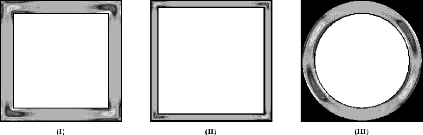
Figure 2:

Figure 3:

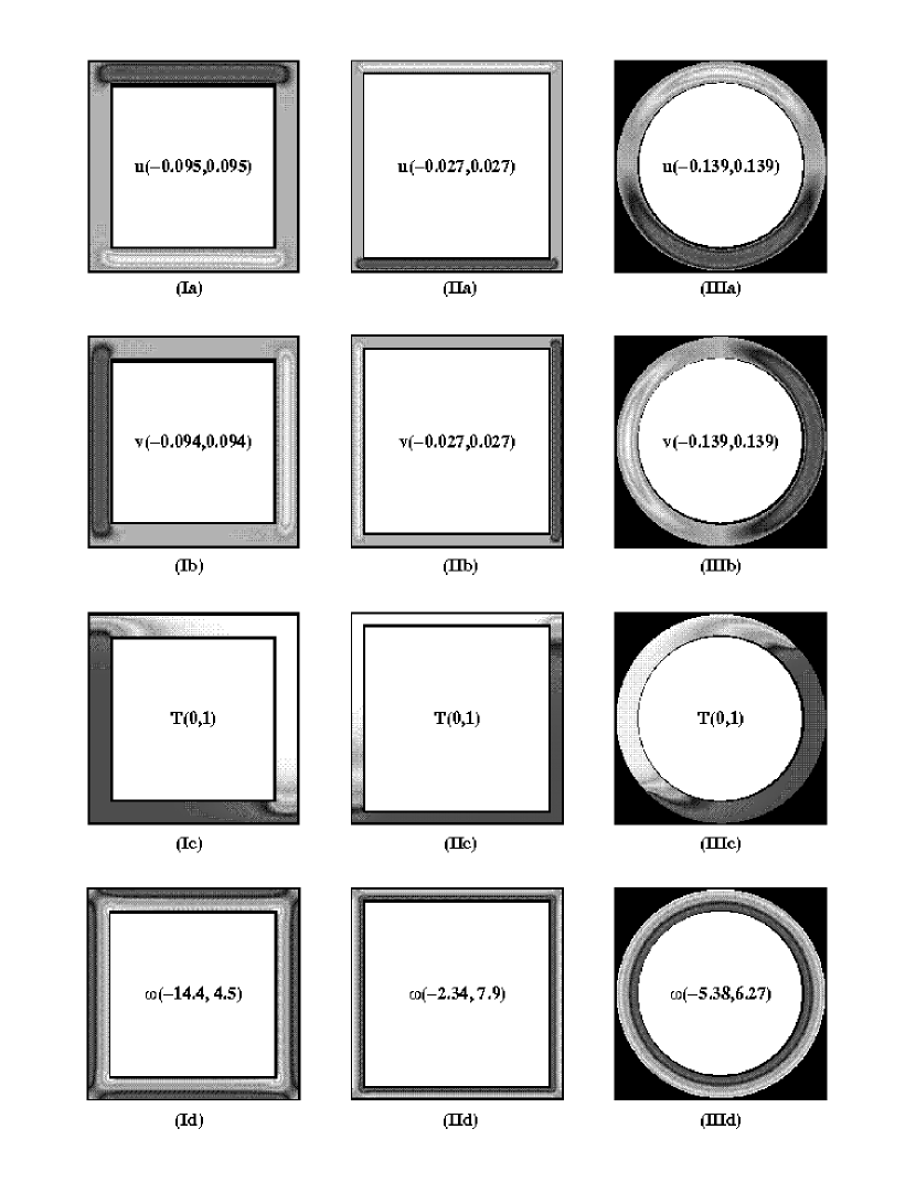
Figure 4:

Figure 5:

Figure 6:

Figure 7:

Figure 8:

Figure 9:

Figure 10:

Figure 11:

Figure 12:

Figure 13:

Figure 14:

Figure 15:

Figure 16:

Figure 17:

Figure 18:

Figure 19:

References

- [1] A. Belmonte, A. Tilgner, and A. Libchaber, “Temperature and velocity boundary layers in turbulent convection”, Phys. Rev. E, 50(1), 269 (1994).
- [2] B. Castaing, G. Gunaratne, F. Heslot, L. Kadanoff, A. Libchaber, S. Thomae, X.Z. Wu, S. Zaleski and G. Zanetti, “Scaling of hard thermal turbulence in Rayleigh-Benard convection, J. Fluid Mech., 204, 1 (1989).
- [3] F. Heslot, B. Castaing and A. Libchaber, “Transition to turbulence in helium gas”, Phys. Rev. A, 36, 5870 (1987).
- [4] G.E. Karniadakis, M. Israeli and S.A. Orszag, “High-Order Splitting Methods for the Incompressible Navier-Stokes Equations”, J. Comput. Phys., 97, 414 (1991).
- [5] J.B. Keller, “Periodic oscillations in a model of thermal convection”, J. Fluid Mech., 29, 599 (1967).
- [6] L.D. Landau and E.M. Lifshitz, “Fluid Mechanics”, 2nd Ed., Pergamon Press, Oxford (1987).
- [7] S.A. Orszag and A.T. Patera, “Secondary instability of wall-bounded shear flows”, J. Fluid Mech., 128, 347 (1983).
- [8] A.T. Patera, “A spectral element method for fluid dynamics; Laminar flow in a channel expansion”, J. Comput. Phys., 54, 468 (1984).
- [9] A.G. Tomboulides, M. Israeli, G.E. Karniadakis, “Efficient removal of boundary-divergence errors in time-splitting methods”, J. Sc. Comp., 4, 291 (1989).
- [10] P. Welander, “On the oscillatory instability of a differentially heated fluid loop”, J. Fluid Mech., 29, 17 (1967).
- [11] X.Z. Wu, ”Along the road to developed turbulence: Free thermal convection in low temperature helium gas”, Ph.D. Dissertation, The University of Chicago (1991).
- [12] X.Z. Wu and A. Libchaber, “Scaling relations in thermal turbulence: The aspect ratio dependence”, Phys. Rev. A, 45(2), 842, (1992).