Periodic-Orbit Theory of Anderson Localization on Graphs

Abstract

We present the first quantum system where Anderson localization is completely described within periodic-orbit theory. The model is a quantum graph analogous to an a-periodic Kronig-Penney model in one dimension. The exact expression for the probability to return of an initially localized state is computed in terms of classical trajectories. It saturates to a finite value due to localization, while the diagonal approximation decays diffusively. Our theory is based on the identification of families of isometric orbits. The coherent periodic-orbit sums within these families, and the summation over all families are performed analytically using advanced combinatorial methods.

Anderson localization is a genuine quantum phenomenon. So far, attempts to study this effect within a semiclassical (periodic-orbit) theory seemed to be doomed to fail from the outset: It is not clear whether the leading semiclassical approximation for the amplitude associated with a single classical orbit is sufficiently accurate. Even more seriously, there is no method available to add coherently the contributions from the exponentially large number of contributing orbits. Here, we address the second problem and develop a method to perform the coherent periodic-orbit (PO) sums in a standard model—a quantum graph analogous to the Kronig-Penney model in 1D—for which the PO theory is exact. For a list of references on the long history of graph models see [1].

For investigating Anderson localization we consider the quantum return probability (RP). It is defined as the mean probability that a wave packet initially localized at a site is at the same site after a given time. We show that the long-time RP approaches a positive constant, which proves that the spectrum has a point-like component with normalizable eigenstates. The asymptotic RP is the inverse participation ratio, which is a standard measure of the degree of localization. The RP can also be seen as 2-point form factor of the local spectrum [2]. As such, it belongs to the class of quantities which can be expressed as double sums over PO’s of the underlying classical dynamics [3]. Because of the exponential proliferation of the PO’s in chaotic systems, the resulting sums are hard to perform. Consequently, most semiclassical approaches to spectral two-point correlations were restricted to the diagonal approximation where the interference between different PO’s is neglected [3, 2, 4, 5, 6]. While this method is very successful for short-time correlations, it fails to reproduce long-time effects such as Anderson localization which are due to quantum interferences. In [7] the universal long-time behavior of the form factor was related to universal classical action correlations between PO’s of a chaotic system. A deeper understanding of how quantum universality is encoded in classical correlations is highly desirable but still lacking, despite some recent progress [8, 9]. This context is our motivation for developing the first PO theory of 1D Anderson localization, although the phenomenon as such is well understood [10, 11, 12, 13, 14].

Quantum graphs exhibit both classical and quantum universal properties, which qualify them as model systems in quantum chaos [1]. The PO theory in graphs is exact. Hence, graphs are well suited for the study of PO correlations and their expected universal features. Recently, we reproduced the complete form factor of the circular unitary ensemble of $2\times 2$ random matrices using a PO expansion in a simple quantum graph [15]. The new combinatorial tools developed there will be used to compute the quantum RP, by extending a method due to Dyson [19] for summing over orbits in a 1D topology.

FIG. 1.: Top: Quantum chain graph with vertices (dots) and bonds (line segments). The arrow shows the initial state used to compute the RP. Bottom: The family $[m_{0},m_{1},m_{2}]=[1,2,2]$ of different but isometric orbits returning after topological time $n=10$ to the vertex $0$.

We consider a quantum graph with a 1D chain topology and use the intuitive notation as indicated in Fig. 1. The bond lengths $L_{j}=x_{j+1}-x_{j}$ are disordered, i. e. pairwise rationally independent. On a bond $j$ the general solution of the 1D Schrödinger equation for wave number $k$ is $\Psi_{j}(x)=a_{j,+}\exp(+{i}\,k[x-x_{j}])+a_{j,-}\exp(-{i}\,k[x-x_{j+1}])$. The matching of solutions across a vertex is achieved in terms of a unitary scattering matrix $\sigma_{j}(r_{j},t_{j})$ such that

$$\pmatrix{a_{j-1,-}\cr a_{j,+}}=\pmatrix{t_{j}&r_{j}\cr r_{j}&t_{j}}\;\pmatrix{{e}^{{i}\,k\,L_{j}}\ a_{j,-}\cr{e}^{{i}\,kL_{j-1}}\ a_{j-1,+}}$$ (1)

The phase factors on the r.h.s. account for the free motion on the bonds. The matrices $\sigma_{j}$ will be assumed independent of $k$ and are parametrized as $r_{j}=i\cos\eta_{j},\ t_{j}=\sin\eta_{j}$. A similar model was used e. g. in the analysis of an optical experiment demonstrating Anderson localization in the transmission of light through a disordered stack of transparent mirrors [16]. The vertex-scattering matrices $\sigma_{j}$ could also be computed by assuming $\delta$-potentials at $x=x_{j}$, as in the Kronig-Penney model [17]. In the following we shall consider two situations: (i) random $\sigma$, where the $\eta_{j}$ are independent random variables distributed such that the corresponding transmission and reflection probabilities $T_{j}=|t_{j}|^{2}$, $R_{j}=|r_{j}|^{2}$ are uniformly distributed in the interval $[0,1]$, and (ii) constant $\sigma$, where $T_{j}=T$, $R_{j}=R$ $\forall\ j$.

At fixed $k$ we consider the Hilbert space of coefficient vectors ${\bf a}\equiv a_{j,v}$ where $j$ goes over the vertices, and $v=\pm$. We introduce a unitary operator

$$U_{j^{\prime},v^{\prime};j,v}(k) = {e}^{{i}\,kL_{j}}\,(\delta_{+v^{\prime},v}\delta_{j^{\prime},j+v}\,t_{j+{v+1\over 2}}+$$ (3)

$$\phantom{{e}^{{i}\,kL_{j}}\,(}\delta_{-v^{\prime},v}\delta_{j^{\prime},j}\,r_{j+{v+1\over 2}})\,.$$

The map defined by $U(k)$ describes the time evolution of a coefficient vector. It is the natural object for the investigation of the graph [1]. $k$ is an eigenvalue of the graph Hamiltonian iff $1$ is in the spectrum of $U(k)$, that is when all the matching conditions (1) can be satisfied simultaneously ${\bf a}=U(k){\bf a}$. In terms of $U$ we can characterize the degree of localization by calculating the averaged quantum RP

$${\cal P}(n)=\left\langle|(U^{n})_{0,+;0,+}|^{2}\right\rangle$$ (4)

as a function of the discrete topological time $n$ of a state which was initially prepared as $a_{j,v}=\delta_{j,0}\delta_{v,+}$ (arrow in Fig. 1, top). The average $\left\langle\dots\right\rangle$ in (4) is over a large $k$ interval, and for random $\sigma$ also over the ensemble of $\sigma$ defined above. Due to the structure of $U$, ${\cal P}(n)\neq 0$ only for even $n=2m$.

The classical analogue of the quantum graph [1] is a Markovian random walk with vertex reflection and transmission probabilities which are equal to the quantum mechanical ones defined above. A classical trajectory is encoded by the sequence of traversed vertices $\{j_{\nu}\}$ which must be consistent with the connectivity of the graph. In our case $v_{\nu}=j_{\nu+1}-j_{\nu}=\pm 1$. Given the initial vertex, a trajectory can also be identified uniquely by the sequence $\{v_{\nu}\}$. Because of the probabilistic nature of the dynamics all trajectories are unstable. In general, the representation of a quantum evolution operator in terms of classical trajectories involves a semiclassical approximation. Here it is exact and amounts simply to expanding the matrix products in (4). The result

$${\cal P}(n)=\left\langle\left|\sum_{\lambda}{\cal A}_{\lambda}\exp({i}\,k{\cal L}_{\lambda})\right|^{2}\right\rangle$$ (5)

can be interpreted in terms of the classical trajectories introduced above. $\lambda$ runs over all trajectories contributing to the RP (4), i. e. all sequences $\{v_{\nu}\}$ ($\nu=0,\dots,n-1$) with $\sum_{\nu}v_{\nu}=0$. The traversed vertices are $j_{\nu}=\sum_{\nu^{\prime}\leq\nu}v_{\nu^{\prime}}$. For graphs, the concepts of returning trajectories and PO’s coincide, hence (5) is a PO sum. The length of an orbit is ${\cal L}_{\lambda}=\sum_{\nu=0}^{n-1}L_{j_{\nu}}$, such that $k{\cal L}_{\lambda}$ is the corresponding action in units of $\hbar$. The amplitude ${\cal A}_{\lambda}$ is the product of the transmission and reflection amplitudes accumulated along the orbit ${\cal A}_{\lambda}=\prod_{\nu=1}^{n}{\cal A}_{\lambda,\nu}$ with ${\cal A}_{\lambda,\nu}=t_{j_{\nu}}$ if $v_{\nu+1}=v_{\nu}$ and ${\cal A}_{\lambda,\nu}=r_{j_{\nu}}$ otherwise. It was shown in [1] that $|{\cal A}_{\lambda}|$ plays the rôle of the stability amplitude of the orbit, while the phase of ${\cal A}_{\lambda}$ is equivalent to the Maslov index.

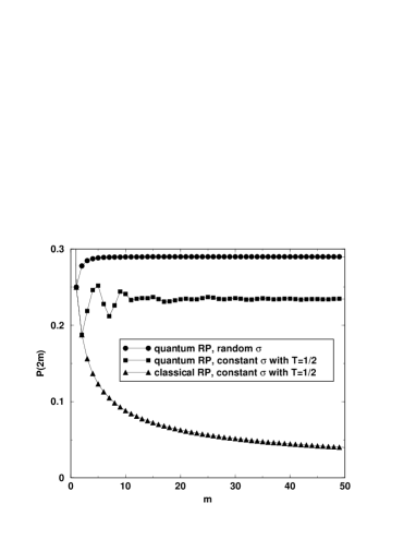
FIG. 2.: Exact quantum and classical return probability ${\cal P}(2m)$ as given by Eqs. (6), (11).

Expanding $\left|\dots\right|^{2}$ in (5) we obtain a double sum over PO’s of the type studied in [3]. For short time, the interference terms pertaining to two different PO’s which are not related by an exact symmetry can be neglected due to the averaging applied. For constant $\sigma$ with $T=R=1/2$ this diagonal approximation simply amounts to counting the number of classical PO’s with period $n=2m$ since all weights $|{\cal A}_{\lambda}|^{2}=2^{-n}$ coincide. Any such PO is represented by a code word $\{v_{\nu}\}$ containing $m$ letters $+$ and $-$, respectively. According to the initial condition $v_{1}=+$. Hence, each PO $\lambda$ in (5) corresponds to a way of selecting from the remaining $n-1$ time steps those $m$ with negative velocity, and we have

$${\cal P}_{\rm cl}(n=2m)={1\over 2^{n}}{n-1\choose n/2}\approx{1\over\sqrt{2n\pi}}\qquad({n\to\infty})$$ (6)

(triangles in Fig. 2). It is well known that the diagonal approximation yields the classical RP [2]. And indeed, for long time (6) shows the expected classical diffusion. The decay of the classical RP to $0$ corresponds to the obvious fact that there is no localization in the classical analogue of our model.

In the following we will show that a constructive interference between PO’s with different number of reflections but equal lengths leads to a finite saturation value of the exact RP and consequently to localization [18]. When (4) is expanded into a double sum, only pairs of orbits with equal lengths survive the $k$ average. Hence, all relevant interferences are confined to families of isometric orbits. Suppose a PO $\lambda$ returning to bond $(0,+)$ after $2m$ collisions with vertices traverses the bonds $(j,+)$ and $(j,-)$ $m_{j}$ times, respectively ($\sum_{j}m_{j}=m$). The length of this PO is ${\cal L}_{\lambda}=2\sum_{j}m_{j}L_{j}$. Thus, for rationally independent bond lengths $L_{j}$ a family of isometric orbits contains all orbits sharing the set ${\cal L}=[m_{0},m_{\pm 1},\dots]$. In contrast to the diagonal approximation, these are not only symmetry-related orbits. A simple example is shown in Fig. 1 (bottom), but with increasing orbit length families can contain more and more PO’s. Taking into account orbit families Eq. (5) becomes

$${\cal P}(n=2m)=\sum_{{\cal L}\in{{\cal F}_{n}}}\left|\sum_{\lambda\in{\cal L}}{\cal A}_{\lambda}\right|^{2}=\sum_{{\cal L}\in{{\cal F}_{n}}}{\cal P}({\cal L})\,.$$ (7)

The outer sum is over the set ${\cal F}_{n}$ of families, while the inner one is a coherent sum over the orbits belonging to a given family. The phase and amplitude of each PO depend on its itinerary. The phase equals the parity of half the number of reflections. Had one assumed that these phases are randomly distributed within a family, (7) would again reduce to the diagonal approximation [20]. In contrast, the exact result derived below from Eq. (7) is shown in Fig. 2. For both, constant and random $\sigma$, the RP saturates to a finite value indicating localization. Hence, quantum localization is due to a delicate and systematic imbalance between positive and negative terms within families. This can be regarded as a classical correlation (deviation from a random distribution) of phases of PO’s. The saturation value, i. e. the inverse participation ratio is expected to be inversely proportional to the localization length and the classical diffusion constant, see e. g. [6] and refs. therein. Indeed we find for constant $\sigma$ and a diffusion constant $D=T/(1-T)\gg 1$ the relation $\lim_{m\to\infty}{\cal P}(2m)=(D\pi)^{-1}$ [20].

In the sequel we outline the analytical evaluation of Eq. (7), deferring a detailed exposé to a subsequent publication [20]. A sum with a similar structure was calculated by Dyson [19] to study a disordered chain of harmonic oscillators. This system is analogous to our model, but Dyson computed a different quantity—the density of states. It is essentially different from the RP because the latter is a two-point correlation function. Dyson computed the traces of powers of a Hermitian matrix, and did not have to keep track of the phases encountered in the computation of diagonal elements of powers of a unitary matrix. Consequently the combinatorial arguments needed to evaluate (7)—though similar in spirit to Dyson’s approach—are quite different from [19].

To start, we consider a one-sided graph with $j\geq 0$, and $R_{0}=1$, and perform the coherent sum over all orbits $\lambda$ in a given family. To keep track of the precise number of reflections for each orbit, we choose to specify the orbit by the segments with positive velocity $v_{\nu}=+$. In the schematic representation of Fig. 1 (bottom) these are the arrows which point to the right. When the left pointing arrows are deleted from the bonds $1$ and $2$ in Fig. 1 (bottom) one obtains the arrow structures displayed in Fig. 3. The vertical displacement of the arrows provides the information about the time ordering which is necessary to reconstruct the complete orbit from the right pointing arrows. The lower an arrow, the later it appears in the trajectory. The number of arrows to the left (right) of the vertex $j$ is $m_{j-1}$ ($m_{j}$). An orbit can be completely specified by prescribing, at all vertices, in which order the adjacent arrows are traversed. Note that this local time order can be chosen independently for each vertex. As a consequence, the factorization

$${\cal P}([m_{0},\dots,m_{b-1}])={\cal V}_{b}(m_{b-1})\prod_{j=1}^{b-1}{\cal V}_{j}(m_{j},m_{j-1})$$ (8)

results. $b$ denotes the rightmost vertex along the orbit, i. e. $m_{j}=0$ $\forall j\geq b$. The local contribution ${\cal V}_{j}(m_{j},m_{j-1})$ from a vertex will be determined in the following.

FIG. 3.: This figure corresponds to vertex 2 in Fig. 1, which is approached twice from the left and from the right. The right pointing arrows can be arranged in 3 distinct ways, which correspond to the 3 decompositions of the number 2 into 2 non-negative integers 2=1+1=0+2=2+0 (left to right).

Each local time order at vertex $j$ corresponds to one of ${m_{j}+m_{j-1}-1\choose m_{j-1}-1}$ possibilities to distribute $m_{j}$ identical objects over $m_{j-1}$ sites, or—in other words—to decompose $m_{j}$ into $m_{j-1}$ non-negative summands (Fig. 3). The number of transmissions to the right at vertex $j$ is given by the number of non-zero terms in this decomposition. We can express ${\cal V}_{j}(m_{j},m_{j-1})$ as a sum taking into account the number $\nu$ of such transmissions, together with the associated amplitude. We obtain

$${\cal V}_{j}=\left|\sum_{\nu}{m_{j-1}\choose\nu}{m_{j}-1\choose\nu-1}t_{j}^{2\nu}\,r_{j}^{m_{j}+m_{j-1}-2\nu}\right|^{2}\,.$$ (9)

The standard definition of binomial coefficients ensures that the sum can be taken over all integers $\nu$. The power of $t_{j}$ in the expansion (9) is $2\nu$ since the number of transmissions to the left and to the right is the same. ${m_{j}-1\choose\nu-1}$ is the number of decompositions of $m_{j}$ into $\nu$ positive summands and ${m_{j-1}\choose\nu}$ corresponds to selecting the $\nu$ non-zero terms from all $m_{j-1}$ summands. The sum in (9) is a special Kravtchouk polynomial—a well-known object in combinatorics [21, 15].

With (8), (9) we can perform the summation over all orbits $\lambda$ of a given family in (7). However, there are $\sum_{b=1}^{m}{m-1\choose b-1}=2^{m-1}$ decompositions of an integer $m$ into positive summands $m_{j}$, i. e. the number of families grows exponentially with time. To sum over all families we derive a recursion relation which dramatically reduces the number of terms needed. Grouping in (7) all terms according to the number of traversals of the first two bonds $m_{0}$ and $m_{1}$, i. e. defining $B_{m}(m_{0},m_{1})=\sum_{m_{2},\dots}{\cal P}([m_{0},m_{1},m_{2},\dots])$, we find $B_{m}(s+1,t)={\cal V}(t,s+1)/{\cal V}(t,s)\,B_{m-1}(s,t)$ for $s\geq 0$ and $B_{m}(1,t)={\cal V}(t,1)\sum_{s=1}^{m-2}B_{m-1}(t,s)$. Summing over the second argument of $B_{m}(s,t)$ we obtain the combined contribution $V_{m}(s)$ from all orbits with period $2m$ which traverse the initial bond exactly $s$ times before finally returning to it. The corresponding recursion relation is

$$V_{m}(t)=\sum_{s=1}^{m-t}{\cal V}(s,t)V_{m-t}(s)\qquad(1\leq t<m)\,.$$ (10)

The recursion is initialized using the elements $V_{m}(m)$, which are due to a single PO: the orbit bouncing $m$ times between the vertices $j=0$ and $j=1$. The RP for the one-sided graph is now ${\cal P}(2m)=\sum_{s=1}^{m}V_{m}(s)$.

For the unrestricted graph a returning trajectory can be composed of simple loops to the right and to the left from the initial bond. Both groups can be described by the results for the one-sided problem. Using similar arguments as in the derivation of (9) we find

$${\cal P}(2m)=\sum_{m_{r}=1}^{m}\sum_{s=1}^{m_{r}}V_{m-m_{r}+s}(s)\,V_{m_{r}}(s)\,.$$ (11)

We were able to solve the recursion (11) analytically for random $\sigma$. After expanding $|\dots|^{2}$ in (9) we get

$$\ {\cal V}_{j}^{\rm(av)}(m_{j},m_{j-1})={1\over 2}\int_{0}^{\pi/2}\!\!\!\!\sin 2\eta_{j}{\rm d}\eta_{j}\,{\cal V}_{j}(m_{j},m_{j-1},\eta_{j})$$ (12)

$$= {m_{j}^{2}\over m_{j-1}+m_{j}+1}\sum_{\nu,\nu^{\prime}}{(-1)^{\nu+\nu^{\prime}}\over\nu\nu^{\prime}}{m_{j-1}+m_{j}\choose\nu+\nu^{\prime}}^{-1}$$ (14)

$$\times{m_{j-1}-1\choose\nu-1}{m_{j}-1\choose\nu-1}{m_{j-1}-1\choose\nu^{\prime}-1}{m_{j}-1\choose\nu^{\prime}-1}$$

$$= {2\,m_{j-1}^{2}\over(m_{j-1}+m_{j}-1)(m_{j-1}+m_{j})(m_{j-1}+m_{j}+1)}\,.$$ (15)

The last equality follows from an identity which we proved previously [15] using recent developments in combinatorial theory [22]. For the outmost vertex on an orbit (15) simplifies to ${\cal P}_{b}^{\rm(av)}(m_{b-1})=1/(m_{b-1}+1)$. Consequently we can initialize the recursion (10) by $V^{\rm(av)}_{m}(m)=1/(m+1)$, which results in $V^{\rm(av)}_{m}(s)=s/(m^{2}+m)$. Summing with respect to $s$ we find that the RP of the one-sided graph is constant ${\cal P}_{\rm os}(2m)=1/2$ for $m>0$. For the unrestricted graph and $m\to\infty$ the double sum in (11) can be approximated by a double integral yielding $\lim_{m\to\infty}{\cal P}(2m)=\pi^{2}/3-3$ which is indeed the saturation value of the top curve in Fig. 2.

In summary, we have shown that Anderson localization can be reproduced from PO theory only when classical correlations are properly taken into account. Here, these correlations show up as exact isometries of families of PO’s, and the non-random distribution of the phases within a family. The failure of the diagonal approximation in a model where PO theory is exact, identifies the neglect of action correlations as the primary source of errors in semiclassical theories of localization and related problems.

Support by the Minerva Center for Nonlinear Physics and the Israel Science Foundation is acknowledged. We thank U. Gavish for valuable comments.

REFERENCES

- [1] T. Kottos and U. Smilansky. Ann. Phys., 274:76, 1999.
- [2] T. Dittrich and U. Smilansky. Nonlinearity, 4:59 (1991).
- [3] M. V. Berry. Proc. R. Soc. London A, 400:229, 1985.
- [4] R. A. Jalabert et. al. Phys. Rev. Lett., 65:2442, 1990.
- [5] N. Argaman et al. Phys. Rev. B, 47:4440, 1993.
- [6] T. Dittrich. Phys. Rep., 271:267, 1996.
- [7] N. Argaman et al. Phys. Rev. Lett., 71:4326, 1993.
- [8] D. Cohen et al. Ann. Phys., 264:108, 1998.
- [9] D. Cohen J. Phys. A, 31:277, 1998.
- [10] N. F. Mott and W. D. Twose. Adv. Phys., 10:107, 1961.
- [11] V. L. Berezinskij. Sov. Phys. JETP, 38:620, 1974.
- [12] D. J. Thouless. Phys. Rev. Lett., 39:1167, 1977.
- [13] E. Abrahams et al. Phys. Rev. Lett., 42:673, 1979.
- [14] T. Kottos et. al. J. Phys. B, 9:1777, 1997.
- [15] H. Schanz and U. Smilansky. chao-dyn/9904007, 1999.
- [16] M. V. Berry and S. Klein. Eur. J. Phys., 18:222, 1997.
- [17] R. Kronig and W. G. Penney. Proc. R. Soc. London A, 130:499, 1931.
- [18] This constructive interference is complementary to the “discordance” (destructive interference) between non-returning rays (trajectories) which was discussed in [16].
- [19] F. J. Dyson. Phys. Rev., 92:1331, 1953.
- [20] H. Schanz and U. Smilansky, to be published.
- [21] A. F. Nikiforov, S. K. Suslov, and V. B. Uvarov. Classical Orthogonal Polynomials of a Discrete Variable. Springer Series in Computational Physics. Springer, Berlin, 1991.
- [22] D. Zeilberger M. Petkovšek, H. S. Wilf. A=B. AK Peters, Wellesley, Massachusetts, 1996.