[

About coherent structures in random shell models for passive scalar advection

Abstract

A study of anomalous scaling in models of passive scalar advection in terms of singular coherent structures is proposed. The stochastic dynamical system considered is a shell model reformulation of Kraichnan model. We extend the method introduced in [1] to the calculation of self-similar instantons and we show how such objects, being the most singular events, are appropriate to capture asymptotic scaling properties of the scalar field. Preliminary results concerning the statistical weight of fluctuations around these optimal configurations are also presented.

]

Experimental and numerical investigation of passive scalars advected by turbulent flows have shown that passive scalar structure functions, $T_{2n}(r)$ have an anomalous power law behaviour : $T_{2n}(r)=\langle(\theta(x+r)-\theta(x))^{2n}\rangle=\langle(\delta_{r}\theta(x))^{2n}\rangle\sim r^{\zeta(2n)}$, where for anomalous scaling we mean that the exponents $\zeta(2n)$ do not follow the dimensional estimate $\zeta(2n)=n\zeta(2)$. A great theoretical challenge is to develop a theory which allows a systematic calculation of $\zeta(n)$ from the Navier-Stokes equations. Recently [2], it has been realized that intermittent power laws are also present in a model of passive scalar advected by stochastic velocity fields, for $n>1$ [3, 4]. The model, introduced by Kraichnan, is defined by the standard advection equation:

$$\partial_{t}\theta+{\bf u}\cdot\mbox{\boldmath$\partial$}\theta=\kappa\Delta\theta+\phi,$$ (1)

where ${\bf u}$ is a Gaussian, isotropic, white-in-time stochastic $d$-dimensional field with a scaling second order structure function: $\langle(u_{i}(x)-u_{i}(x+r))(u_{j}(x)-u_{j}(x+r))\rangle=D_{0}r^{\xi}((d+\xi-1)\delta_{ij}-\xi r_{i}r_{j}/r^{2})$. The physical range for the scaling parameter of the velocity field is $0\leq\xi\leq 2$, $\phi$ is an external forcing and $\kappa$ is the molecular diffusivity.
A huge amount of work has been done in the last years on the Kraichnan model. Due to the white-in-time character of the advecting velocity field, the equation for passive correlators of any order $n$ are linear and closed. This allows explicit, perturbative calculations of anomalous exponents in terms of zero-mode solutions of the closed equation satisfied by $n$-points correlation function, by means of developments in $\xi$ [3] or in $1/d$ [4], with $d$ the physical space dimensionality.
The connection between anomalous scaling and zero modes, if fascinating from one side, looks very difficult to be useful for the most important problem of Navier-Stokes eqs. In that case, being the problem non linear, the hierarchy of equations of motion for velocity correlators is not closed and the zero-mode approach should be pursued in a much less handable functional space.
From a phenomenological point of view, a simple way to understand the presence of anomalous scaling is to think at the scalar field as made of singular scaling fluctuations $\delta_{r}\theta(x)\sim r^{h(x)}$, with a probability to develop an $h$-fluctuation at scale $r$ given by $P_{r}(h)\sim r^{f(h)}$, being $f(h)$ the co-dimension of the fractal set where $h(x)=h$. This is the multifractal road to anomalous exponents [7] that leads to the usual saddle-point estimate for the scaling exponents of structure functions: $\zeta(2n)=\min_{h}{(2nh+f(h))}$ [8]. In this framework, high order structure functions are dominated by the most intense events, i.e. fluctuation characterized by an exponent $h_{min}$: $\lim_{n\rightarrow\infty}\zeta(n)=nh_{min}$. The emergence of singular fluctuations, at the basis of the multifractal interpretation, naturally suggests that instantonic calculus can be used to study such special configurations in the system. Recently, instantons have been successfully applied in the Kraichnan model to estimate the behaviour of high-order structure functions when $d(2-\xi)\gg 1$ [5], and to estimate PDF tails for $\xi=2$ [6].
In this letter, we propose an application of the instantonic approach in random shell models for passive scalar advection, where explicit calculation of the singular coherent structures can be performed.
Let us briefly summarized our strategy and our main findings. First, we restrict our hunt for instantons to coupled, self-similar, configurations of noise and passive scalar, a plausible assumption in view of the multifractal picture described above. We develop a method for computing in a numerical but exact way such configurations of optimal Gaussian weight for any scaling exponent $h$. We find that $h$ cannot go below some finite threshold $h_{min}(\xi)$. We compare $h_{min}(\xi)$ at varying $\xi$ given from the instantonic calculus with those extracted from numerical simulation showing that the agreement is perfect and therefore supporting the idea that self-similar structures gouvern high-order intermittency.
Second, assuming that these localized pulse-like instantons constitute the elementary bricks of intermittency also for finite-order moments we compute their dressing by quadratic fluctuations. We obtain in this way the first two terms of the function $f(h)$ via a “semi-classical” expansion. Let us notice that a rigorous application of the semi-classical analysis would demand for a small parameter controlling the rate of convergence of the expansion, like $1/n$ where $n$ is the order of the moment [6] or $1/d$, where $d$ is the physical space dimension[5]. As we do not dispose of such small parameter in our problem, the reliability of our results concerning the statistical weight of the $h$-pulses can only be checked from an a posteriori comparison with numerical data existing in literature. At the end of this communication, we will present some preliminary results on such important issue, while much more extensive work will be reported elsewhere.
Shell models are simplified dynamical models which have demonstrated in the past to be able to reproduce many of the most important features of both velocity and passive turbulent cascades [8].
The model we are going to use is defined as follows. First, a shell-discretization of the Fourier space in a set of wavenumbers defined on a geometric progression $k_{m}=k_{0}\lambda^{m}$ is introduced. Then, passive increments at scale $r_{m}=k_{m}^{-1}$ are described by a real variable $\theta_{m}(t)$. The time evolution is obtained according to the following criteria : (i) the linear term is purely diffusive and is given by $-\kappa k_{m}^{2}\theta_{m}$; (ii) the advection term is a combination of the form $k_{m}\theta_{m^{\prime}}u_{m^{\prime\prime}}$, where $u_{m}$ are random Gaussian and white-in-time shell-velocity fields; (iii) interacting shells are restricted to nearest-neighbors of $m$; (iv) in the absence of forcing and damping, the model conserves the volume in the phase-space and the energy $E=\sum_{m}|\theta_{m}|^{2}$. Properties (i), (ii) and and (iv) are valid also for the original equation (1) in the Fourier space, while property (iii) is an assumption of locality of interactions among modes, which is rather well founded as long as $0\ll\xi\ll 2$. The simplest model exhibiting inertial-range intermittency is defined by [9]:

$$[\frac{d}{dt}+\kappa k_{m}^{2}]\,\theta_{m}(t)=c_{m}\theta_{m-1}(t)u_{m}(t)+$$ (2)

$$+a_{m}\theta_{m-1}(t)u_{m-1}(t)+\delta_{1m}\phi(t),$$ (3)

with $a_{m}=-c_{m-1}=k_{m}$, and where the forcing term acts only on the first shell. Following Kraichnan, we also assume that the forcing term $\phi(t)$ and the velocity variables $u_{m}(t)$ are independent Gaussian and white-in-time random variables, with the following scaling prescription for the advecting field:

$$\langle u_{m}(t)u_{n}(t^{\prime})\rangle=\delta(t-t^{\prime})k_{m}^{-\xi}\delta_{mn}.$$ (4)

Shell models have been proved analytically and non-perturbatively [9] to possess anomalous zero modes similarly to the original Kraichnan model (1).
The role played by fluctuations with local exponent $h(x)$ in the original physical space model is here replaced by the formation at larger scale of structures propagating self-similarly towards smaller scales. The existence in the inviscid unforced problem of such solutions associated with the appearance of finite time singularities is a The analytical resolution of the instantonic problem even in the simplified case of shell models is a hard task. In [1], a numerical method to select self-similar instantons in the case of a shell model for turbulence, has been introduced. In the following, we are going to apply a similar method to our case.
We rewrite model (3) in a more concise form:

$$\frac{d\mbox{\boldmath$\theta$}}{dt}={\rm M}[{\bf b}]\mbox{\boldmath$\theta$}.$$ (5)

The scalar and velocity gradient vectors, $\theta$ and ${\bf b}$, are made from the variables $\theta_{m}$ and $k_{m}u_{m}$. As far as inertial scaling is concerned, we expect that some strong universality properties apply with respect to the large scale forcing. Indeed, forcing changes only the probability with which a pulse appears at large scale, but not its inertial range scaling behaviour, $P_{k_{m}}(h)\sim k_{m}^{-f(h)}$. So, as we are interested only in the evaluation of $f(h)$, we drop the forcing and dissipation in (5). The matrix ${\rm M}[{\bf b}]$ is linear in ${\bf b}$ and can be obviously deduced from (3). The stochastic multiplicative equation (5) must be interpreted à la Stratonovich. Nevertheless, once the Ito-prescription for time discretization is adopted, the dynamics gets Markovian and a path integral formulation can then be easily implemented. This changes (5) into:

$$\frac{d\mbox{\boldmath$\theta$}}{dt}=-B{\rm D}\mbox{\boldmath$\theta$}+{\rm M}[{\bf b}]\mbox{\boldmath$\theta$},$$ (6)

where ${\rm D}$ is a diagonal matrix (Ito-drift) ${\rm D}_{mm}=k_{m}^{2-\xi}$, and $B$ is a positive constant.
As we said before, we are looking for coherent structures developing a scaling law $\theta_{m}\sim k_{m}^{-h}$ as they propagate towards small scales in the presence of a velocity realization of optimal Gaussian weight. The probability to go from one point to another in configuration space (spanned by $\theta$) between times $t_{i}$ and $t_{f}$ can be written quite generally as a path integral over the three fields ${\bf b}$, $\theta$, $p$ of the exponential $e^{-S[{\bf b},\mbox{\boldmath$\theta$},\mbox{\boldmath$p$}]}=e^{-\int_{t_{i}}^{t_{\!f}}{\cal L}[{\bf b},\mbox{\boldmath$\theta$},\mbox{\boldmath$p$}]dt}$, where the Lagrangian ${\cal L}$ is given by the equation:

$${\cal L}({\bf b},\mbox{\boldmath$\theta$},\mbox{\boldmath$p$})=\frac{1}{2}{\bf b}.{\rm D}^{-1}{\bf b}+\mbox{\boldmath$p$}.(\frac{d\mbox{\boldmath$\theta$}}{dt}+B{\rm D}\mbox{\boldmath$\theta$}-{\rm M}[{\bf b}]\mbox{\boldmath$\theta$}),$$ (7)

and $p$ is an auxiliary field conjugated to $\theta$ which enforces the equation of motion (6). The minimization of the effective action $S$ leads to the following coupled equations:

$$\frac{d\mbox{\boldmath$\theta$}}{dt} = -B{\rm D}\mbox{\boldmath$\theta$}+{\rm M}[{\bf b}]\mbox{\boldmath$\theta$},$$ (8)

$$\frac{d\mbox{\boldmath$p$}}{dt} = B{\rm D}\mbox{\boldmath$p$}-\,^{t}{\rm M}[{\bf b}]\mbox{\boldmath$p$},$$ (9)

with the self-consistency condition for ${\bf b}$:

$${\bf b}={\rm D}\,^{t}{\rm N}[\mbox{\boldmath$\theta$}]\mbox{\boldmath$p$},$$ (10)

where the matrix ${\rm N}[\mbox{\boldmath$\theta$}]$ is defined implicitly through the relation ${\rm N}[\mbox{\boldmath$\theta$}]{\bf b}={\rm M}[{\bf b}]\mbox{\boldmath$\theta$}$.
We are now able to predict the scaling dependence of variables $b_{m}$. For a truly self-similar propagation, the cost in action per each step along the cascade must be constant. The characteristic turn-over time required by a pulse localized on the $m-th$ shell to move to the next one can be dimensionally estimated as $1/(u_{m}k_{m})\equiv b_{m}^{-1}$. Recalling the scaling dependence of ${\rm D}$ and the definition of action (7), we expect: $\Delta S=\int_{t_{m}}^{t_{m+1}}{\cal L}dt\sim k_{m}^{-(2-\xi)}b_{m}$. We can thus deduce that $b_{m}\sim k_{m}^{2-\xi}$.
Let us now discuss how to explicitly find solutions of the above system of equations. Clearly, there is no hope to analytically find the exact solutions of these deterministic non linear coupled equations. Also numerically, the problem is quite delicate, because (8) and (9) are obviously dual of each other and have opposite dynamical stability properties. This phenomenon can be hardly captured by a direct time integration. To overcome this obstacle, in [1] it has been proposed a general alternative scheme which adopts an iterative procedure. For a given configuration of the noise, each step consists in integrating the dynamics of the passive scalar (8) forward in time to let emerge the solution of optimal growth. Conversely, the dual dynamics of the auxiliary field (9) is integrated backward in time, along the direction of minimal growth in agreement with the prediction deduced from (10): $\|\mbox{\boldmath$p$}\|\sim\|\mbox{\boldmath$\theta$}\|^{-1}$. Then the noise ${\bf b}$ can be recomputed by the self-consistency equation (10) and the process is repeated until the convergence is reached.
Self-similar passive solutions must be triggered by self-similar noise configuration:

$$b_{m}(t)=\frac{1}{(t^{*}-t)}F(k_{m}^{2-\xi}(t^{*}-t)),$$ (11)

where $t^{*}$ is the critical time at which a self-similar solution reaches infinitesimally small scales in absence of dissipation. To overcome the non-homogeneity of time evolution seen by these accelerating pulses, we introduce a new time variable $\tau=-\log(t^{*}-t)$. Then, the advecting self similar velocity field (11) can be rewritten under the form: ${\bf b(\tau)}=e^{\tau}{\bf C(\tau)}$ where $C_{m}(\tau)$ is still the velocity gradient field, but expressed in a different time scale, such that: $C_{m}(\tau)=F(m\,(2-\xi)\log\lambda-\tau)$.
The sought self-similar solutions appear in this representation as traveling waves, whose period $T=(2-\xi)\log\lambda$ is fixed by the scaling consideration reported above. In this way, we can limit the search of solutions on the time interval [$0-T$], and the action at the final time $t_{f}=mT$ is deduced by $S({t_{f}})=mS(T)$.
Then comes the main point of our algorithm. For a fixed noise configuration ${\bf C}$, the field $\theta$ must be the eigenvector associated to the maximal (in absolute value) Lyapunov exponent $\sigma_{max}$ of the Floquet evolution operator:

$$U(T;0)={\cal T}_{-1}\,\exp\,\int_{0}^{T}(-B{\rm D}e^{-\tau}+{\rm M}[{\bf C(\tau)}])d\tau.$$ (12)

Here ${\cal T}_{-1}$ denotes the translation operator by one unit to the left along the lattice. Similarly, the auxiliary field must be the eigenvector associated with the Lyapunov exponent $-\sigma_{max}$ of the inverse dual operator ${}^{t}U^{-1}$.
Starting from an initial arbitrary traveling wave shape for ${\bf C}(\tau)$ with period $T$, we have computed the passive scalar and its conjugate fields at any time between $0$ and $T$, by diagonalization of operator $U$, recomputed the velocity gradient field ${\bf C(\tau)}$ from the self-consistency equation (10) and iterated this procedure until an asymptotic stable state, $\theta^{0}$, $p^{0}$, ${\bf C^{0}}$, was reached. The scaling exponent $\theta_{m}\sim k_{m}^{-h}$ for the passive scalar can be deduced by $\theta^{0}_{m}(h)\sim e^{m\sigma_{max}T}$, so that $h=(\xi-2)\sigma_{max}$. Note that $h$ is bound to be positive due to the conservation of energy. In our algorithm, the norm of the gradient velocity field ${\bf C}(0)$ acts as the unique control parameter in a one to one correspondence with $h$. The action $S^{0}(h)$ is, in multifractal language, nothing but the first estimate of $f(h)$ curve based only on the contribution of all pulse-like solutions, more precisely $f(h)=S^{0}(h)/ln\lambda$.
We now turn to the presentation and discussion of our main result. By varying the control parameter, we obtain a continuum of exponents in the range $h_{min}(\xi)\leq h\leq h_{max}(\xi)$. The simple analysis of the $h$-spectrum allows predictions only for observable which do not depend on the $f(h)$ curve, i.e. only on the scaling of $T_{2n}$ for $n\rightarrow\infty$, ($\zeta(n)\sim h_{min}n$ for $n$ large enough).
Unfortunately, high order exponents are the most difficult quantities to be extracted from numerical or experimental data. Nevertheless, thanks to the extreme simplicity of shell models, very accurate numerical simulations have been done [12] at different values of $\xi$ and in some cases a safe upper bound prediction on the asymptotic of $\zeta(n)$ exponents could be extracted.

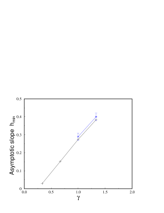
FIG. 1.: Behavior of the asymptotic slope $h_{min}$ as function of $\gamma=2-\xi$ : $(+)$ results from the instantonic calculus for the model of Ref. [12] , $(*)$ upper bound value for $h_{min}$ as extracted from numerical integration of the same model.

To compare our results with the numerical data existing in literature, we have analyzed the shell-model version of passive advection proposed in [12]. In Fig.1, we show the $h_{min}$ curve obtained at various $\xi$ from instantonic calculation, together with the $h_{min}^{num}$ values extracted from direct numerical simulation of the quoted model [12] performed at two different values of $\xi$: the agreement is good. Our calculation predicts, within numerical errors, the existence of a critical $\xi_{c}\sim 1.75$ above which the minimal exponent reaches the lowest bound $h_{min}=0$.
This goes under the name of saturation and it is the signature of the presence of discontinuous-like solutions in the physical space $\delta_{r}\theta\sim r^{0}$. Theoretical [5] and numerical [13] results suggest the existence of such effect in the Kraichnan model for any value of $\xi$. The existence of saturation in this last is due to typical real-space effects and therefore it is not surprising that there in not a complete quantitative analogy with the shell-model case.
Let us now present the other -preliminary- result, i.e. the role played by instantons for finite-order structure functions. If we just keep the zero-th order approximation for $f(h)=S_{0}(h)/\log{\lambda}$, we get the $\zeta_{n}$ curve shown in Fig.2, which is quite far from the numerical results of [14] (the asymptotic linear behavior is in fact not even reached in the range of $n$ represented on the figure). In order to get a better assessment of the true statistical weight of the optimal solutions, we computed the next to leading order term in a “semi-classical” expansion. Fluctuations around the action were developed to quadratic order with respect to $\theta^{0}$, $p^{0}$, ${\bf C^{0}}$, and the summation over all perturbed trajectories leading to the same effective scaling exponent for the $\theta$ field after $m$ cascade steps was performed. It turns out (see Fig.2) that the contribution in the action of quadratic fluctuations, $S_{1}(h)$, greatly improves the evaluation of $\zeta(n)$.

FIG. 2.: Exponents $\zeta_{n}$ of structure functions of order $n$ vs $n$ for $\xi=1$ : ($*$) data from direct numerical simulation of Ref. [14]; $(+)$ Legendre transform of the action $f(h)=S_{0}$; ($\bullet$) Legendre transform of the action $f(h)=S_{0}+S_{1}$. The solid line corresponds to the dimensional scaling.

Naturally, in the absence of any small parameter in the problem, we cannot take for granted that the next correction(s) would not spoil this rather nice agreement with numerical data. But the surprising fact that $S_{0}+S_{1}$ is strongly reduced with respect to $S_{0}$, even for the most intense events, does not imply by itself a lack of consistency of our computation. In any case, the prediction of the asymptotic slope of the $\zeta_{n}$ curve, based on the value $h_{min}$ is obviously valid beyond all orders of perturbation.
Moreover, for values of $\xi>1$, we find that the second order exponent extracted from our calculation is in good agreement the exact result $\zeta_{2}=2-\xi$, suggesting that our approach is able to give relevant statistical information also on not too intense fluctuations.
In conclusion, we have presented an application of the semi-classical approach in the framework of shell models for random advection of passive scalar fields. Instantons are calculated through a numerically assisted method solving the equations coming from probability extrema: the algorithm has revealed capable to pick up those configurations giving the main contributions to high order moments. Of course, we are far from having a systematic, under analytical control, approach to calculate anomalous exponents in this class of models. Nevertheless, the encouraging results here presented raise some relevant questions which go well beyond the realm of shell-models. To quote just one, we still lack a full comprehension of the connection between the usual multiplicative-random process and the instantonic approaches to multifractality: in particular, it is not clear what would be the prediction for multi-scale and multi-time correlations of the kind discussed in [15] within the instantonic formulation.
It is a pleasure to thank J-L. Gilson and P. Muratore-Ginanneschi for many useful discussions on the subject. LB has been partially supported by INFM (PRA-TURBO) and by the EU contract FMRX-CT98-0175.

REFERENCES

- [1] I. Daumont,T. Dombre and J.-L. Gilson, e-Print archive chao-dyn/9905017.
- [2] R.H. Kraichnan, Phys. Rev. Lett. 72, 1016 (1994).
- [3] K. Gawedzki and A. Kupianen, Phys. Rev. Lett. 75, 3608 (1995).
- [4] M. Chertkov, G. Falkovich, I. Kolokolov and V. Lebedev, Phys. Rev. E 52, 4924 (1995).
- [5] E. Balkovsky and V. Lebedev, Phys. Rev. E 58, 5776 (1998).
- [6] G. Falkovich, I. Kolokolov, V. Lebedev and A. Migdal, Phys. Rev. E 54, 4896 (1996).
- [7] U. Frisch, Turbulence: The legacy of A. N. Kolmogorov, Cambridge University Press, Cambridge (1995).
- [8] T. Bohr, M.H. Jensen, G. Paladin and A. Vulpiani Dynamical system approach to turbulence, Cambridge University Press, Cambridge (1998).
- [9] R. Benzi, L. Biferale and A. Wirth, Phys. Rev. Lett. 78, 26 (1997).
- [10] G. Parisi, A Mechanism for Intermittency in a Cascade Model for Turbulence’, unpublished (1990).
- [11] T. Dombre and J.-L. Gilson, Physica D 111, 265 (1998)
- [12] L. Biferale and A. Wirth, Phys. Rev. E 54, 4892, (1996).
-
[13]
U. Frisch, A. Mazzino and M. Vergassola,
Phys. Chem. Earth, in press (1999). - [14] L. Biferale and A. Wirth, Lecture Notes 491, p. 65 (1997).
- [15] L. Biferale, G. Boffetta, A. Celani and F. Toschi, Physica D 127 187 (1999).