TRANSPORT IN PERTURBED
INTEGRABLE HAMILTONIAN SYSTEMS
AND THE FRACTALITY OF PHASE SPACE

Abstract

Hamiltonian systems – diffusion – fractality – Lyapunov numbers

1 Introduction

Transport in phase space is an interesting theoretical aspect of chaotic behaviour in perturbed integrable Hamiltonian systems, since it is encountered in many problems of physical interest (e.g. see Kaneko and Konishi 1989, Meiss 1992, Shlesinger et al. 1993, Benkadda et al. 1994 and references therein). Recently, in a series of papers by Lecar et al. (e.g. see Murison et al. 1994 and references therein), a correlation was reported between transport in action space of the Elliptical Restricted Three Body Problem (ERTBP) and the Lyapunov Characteristic Numbers (LCN’s). In particular the authors, using as a model the ERTBP, presented numerical evidence for the existence of a power law, relating the exit times of asteroidal trajectories from action space regions with the corresponding LCN’s of the trajectories. A theoretical interpretation of this correlation, in cases of ”strong” perturbation, where the motion can be considered as a random walk in action space, has been attempted by Varvoglis and Anastasiadis (1996) and Morbidelli and Froeschlé (1996).

However, in attempting a statistical description of the process, in order to relate the local rate of trajectory divergence to transport, there are two important problems that have to be solved. The first refers to the difficulty in calculating reliably LCN’s in cases where a trajectory is continuously migrating to new regions of phase space, so that the usual method of calculating LCN’s (as the limit of $\chi(t)=ln(\xi/\xi_{0})/t,t\to\infty$) does not show signs of convergence. The second refers to the fact that, in the case of the main asteroidal belt, the perturbation to the motion of asteroids by Jupiter cannot be considered as ”strong”. Both problems originate from the fact that the invariant tori in the regions of interest are far from being completely destroyed, so that the phase space is characterised by a pronounced fractality. This, in turn, implies that transport (i) obeys Levy rather than classical Brownian kinetics (e.g. Shlesinger et al. 1993, Benkadda et al. 1994) and (ii) cannot be considered as a random walk, since it is not a pure Markovian process (there exist long tails in the autocorrelation function, e.g. see Meiss et al. 1983, Meiss 1992 and references therein). Therefore, if one wants to recover theoretically a law analogous to that of Lecar et al. in cases where the perturbation is not strong, he has: (a) to circumvent the problems in the convergence of the function $\chi(t)$ and (b) to take into account the non-Brownian and, possibly, non- Markovian nature of transport in the statistical description of the process.

In this paper we discuss both problems. We use a method for the study of transport in Hamiltonian systems proposed by Varvoglis et al. (1995) in order to calculate the fractality of phase space of the model Hamiltonian

$$H={1\over 2}p_{x}^{2}+{1\over 2}p_{y}^{2}+{1\over 2}p_{z}^{2}+{1\over 2}Ax^{2}+{1\over 2}By^{2}+{1\over 2}Cz^{2}-\epsilon xz^{2}-\eta yz^{2}$$ (1)

for the particular case $A$ = 0.9, $B$ = 0.4, $C$ = 0.225, $\epsilon$ = .56, $\eta$ = 0.20 and $h$ = 0.00765 which has been studied extensively by Contopoulos and Barbanis (1989, 1995) and Barbanis et al. (1997). We conjecture that the fractality may be correlated to the evolution of the function $\chi(t)$ and we discuss the possible usefulness of a “Local Lyapunov time” of a trajectory, in accordance to the ideas of Benkadda et al. (1994) and Morbidelli (1997).

In order to study transport in the phase space of the Hamiltonian (1) we work as follows. We construct a six-dimensional grid in phase space and we calculate the phase space volume, $V(t)$, of the elementary cells explored by a trajectory up to time $t$. All numerically integrated trajectories start on the $z=0$ plane with an initial velocity perpendicular to it ($p_{x}=p_{y}=0$ and $p_{z}$ calculated from the integral of energy). A typical example of the evolution of $V(t)$ for three trajectories, a ”central” one and two adjacent with $x_{0}$ differing by $\Delta x=\pm 10^{-7}$, is given in Fig. 1. We see that, in accordance to its definition, $V(t)$ is the superposition of ”step functions” and we note that these ”steps” seem to have sizes of widely different values. We interpret the form of $V(t)$ as follows. Consecutive small steps indicate that the trajectory is diffusing slowly, according to the ”brownian” model of random walk, in a phase space region characterised by common properties and, in particular, by a common rate of separation, implying a well defined LCN. A ”large” step indicates that the trajectory has moved to an adjacent phase space region with different properties.

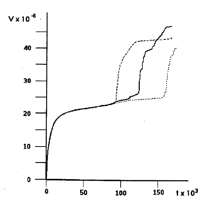
Figure 1: The function $V(t)$ for three trajectories with initial conditions $y_{0}$ = 0.032 and $x_{0}$ = 0.01725 (dotted curve), $x_{0}$ = 0.0172499 (solid curve) and $x_{0}$ = 0.0172501 (dashed curve).

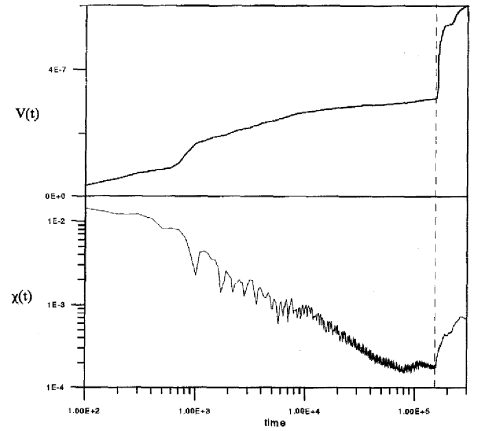
Figure 2: Plots of $V(t)$ and $\chi(t)$ for the ”central” trajectory of Fig. 1 (dotted curve).

2 Results

We test this interpretation by plotting simultaneously the functions $V(t)$ and $\chi(t)$. A typical example of our results is presented in Fig. 2, where we have plotted the above functions for the ”central” trajectory of Fig. 1. We see that, up to $t_{1}\approx 1\cdot 10^{5}$, the trajectory moves in a phase space region whose volume increases slowly with time. From this segment one would infer that the LCN is close to zero, since the corresponding function $\chi(t)$ decays almost exponentially. After $t_{1}$, however, the trajectory migrates suddenly to a region ”outside” the initial one and the function $\chi(t)$ does not show signs of levelling off up to the end of our numerical calculations, at $t_{fin}=3\cdot 10^{5}$. Aside from the fact that this picture corroborates our conjecture, concerning the relation between the transport process and the evolution of $\chi(t)$, Fig. 2 is an example of the practical difficulties arising in the numerical calculation of LCN’s: the limiting behaviour of $\chi(t)$ is governed by the properties of the ”outside” regions of phase space and, therefore, it does not reflect the properties of the initial region where the trajectory started. In the next section we discuss how these difficulties can be circumvented by the definition of a suitable “Local Lyapunov time”.

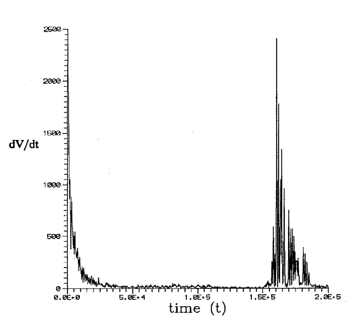
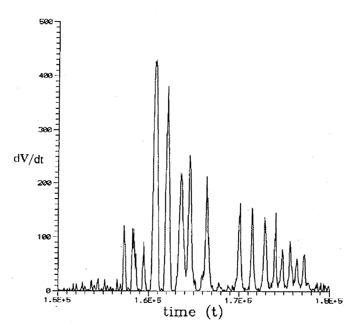
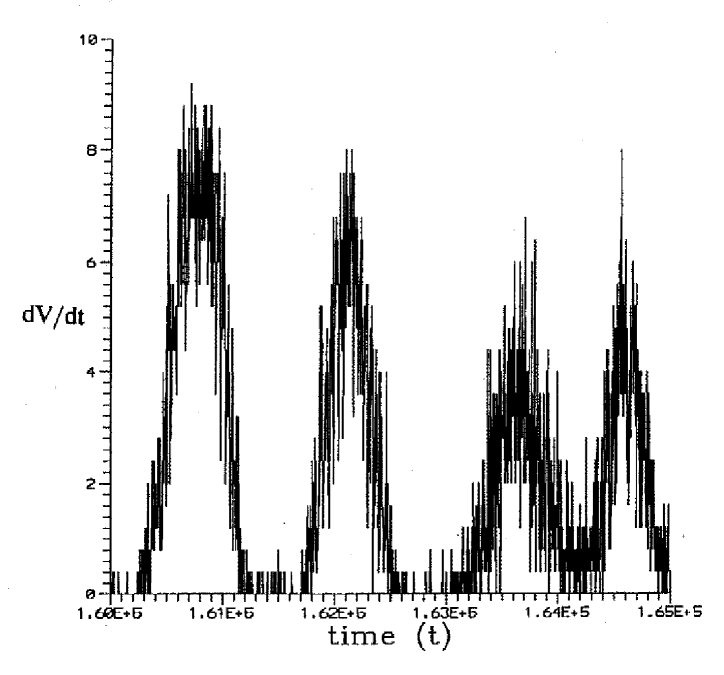
Figure 3: (3a) Plot of $dV/dt$ of the trajectory of Fig. 2. (3b) A magnification of Fig. 3a. (3c) A magnification of Fig. (3b).

Proceeding now to the second problem mentioned, we note that, if the phase space has a fractal structure, then the function $V(t)$ should show some sort of self-similarity. However the time series describing numerically $V(t)$ cannot be used in a fractal analysis algorithm, since it is not stationary (i.e. it shows long-range changes in the mean level). Therefore we decided to use instead its derivative, $dV/dt$, which has the above property. We see that, indeed, $dV/dt$ consists of ”spikes” of all orders, each one corresponding to a ”jump” in $V(t)$ (Figs. 3). After a transient of large spikes, corresponding to the ”spreading” of the trajectory in the initially available phase space region, the value of the function drops until $t\approx 1.5\cdot 10^{5}$, where from the ”forest” of high ”spikes” it is obvious that the trajectory migrates to a nearby phase space region. A closer examination reveals that the spikes possess a prominent self- similar structure: consecutive magnifications of an interval of $dV/dt$ show that each individual spike consists of higher order spikes, down to a scale size corresponding to the 6-D volume of an elementary cell (Figs. 3b and 3c). However, apart from this qualitative approach, we can obtain a quantitative measure of the ”fractality” of the function $dV/dt$ through the calculation of its generalised dimensions, $D(q)$, q = 0, 1, 2, … (e.g. see Schuster, 1988; McCauley, 1995). In particular $D(2)$ is the correlation dimension. A value of $D(2)=1$ implies total randomness, while a value of $D(2)=0$ complete predictability.. It should be noted that the canonical variables $q_{i}(t),p_{i}(t)$ (or any function of them) are not useful for the study of phase space fractality, since the corresponding sets are ”fat fractals” (Benettin et al., 1986).

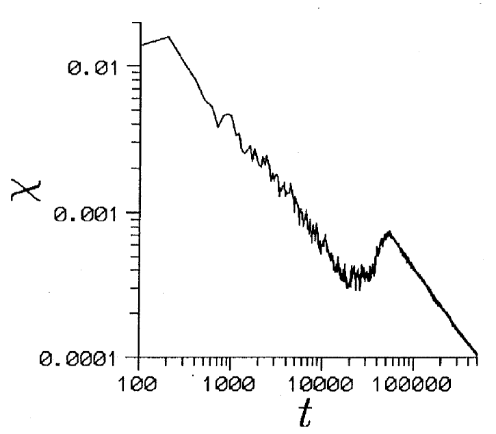
Figure 4: Plot of $\chi(t)$ for a trajectory with initial conditions $x_{0}$ = 0.0095 and $y_{0}$ = 0.0415.

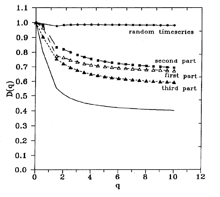
Figure 5: The $D(q)$-spectrum of the trajectory of Fig. 4 (solid curve) as well as that of the three segments described in the text.

From the calculation of the $D(q)$ spectrum we find that $0<D(2)<1$ (Fig. 5), which corroborates the results of the qualitative analysis, showing that $dV/dt$ is a multifractal (for a definition see the Appendix). Moreover it shows that the transport process is not completely random. From the simultaneous plotting of $V(t)$, $dV/dt$, $\chi(t)$ and $D(2)$ for numerous trajectories and segments of them we found that, as a rule, $D(2)$ shows a correlation with $\chi(t)$. In particular the segments of $dV/dt$, corresponding to time intervals where $\chi(t)$ decays, have values of $D(2)$ lower than those of the segments of $dV/dt$, corresponding to time intervals where $\chi(t)$ increases. On the other hand, if the trajectory is treated as a whole, the resulting value of $D(2)$ takes an intermediate value. This fact is in agreement with our interpretation, since, in places where the divergence of trajectories is almost linear with time, we have weak chaos and, therefore, a low correlation dimension. In contrast, in regions where the divergence of trajectories in exponential, we have strong chaos and, therefore, a high correlation dimension.

However this is not always the case. An interesting example is given in Figs. 4 and 5. In Fig. 4 we give the function $\chi(t)$ for a trajectory with initial conditions $x_{0}$ = 0.0095 and $y_{0}$ = 0.0415. We see that three different trajectory segments may be defined: one for the time interval $0<t<2\cdot 10^{4}$, one for $2\cdot 10^{4}<t<6\cdot 10^{4}$ and one for $6\cdot 10^{4}<t<5\cdot 10^{5}$. In the first and third segments $\chi(t)$ shows an almost exponential decay, a typical behaviour of a weakly chaotic trajectory, while in the second segment it shows a steep increase, characteristic of strong chaos. From what has been said above, the trajectory has migrated from one region characterised by an almost linear divergence of trajectories to another one with the same property, passing briefly through a region characterised by an exponential divergence. In Fig. 5 we give the $D(q)$-spectra of the three segments and of the trajectory as a whole. We see that, considering only the three segments, the ”typical” relation, discussed above, between $\chi(t)$ and $D(2)$ still holds. However in this case the $D(2)$ of the trajectory as a whole is considerably lower. This implies that, even while the trajectory has drifted from a phase space region of weak chaos to another, going through one with prominent chaotic behaviour, the third segment of the trajectory ”keeps a memory” of the first, which shows that the process in the second segment is not Markovian!

3 Discussion

In a perturbed integrable Hamiltonian system we can distinguish three regimes, according to the ”amplitude” of the perturbation: those of ”small”, ”medium” or ”large” perturbations, where the ”amplitude” of the perturbation is inferred by the dominant properties of the transport mechanism. In the regime of small perturbation, transport is expected to be governed by Arnold diffusion, as discussed recently by Morbidelli and Froeschlé (1996). In the regime of ”strong” perturbation the following analytic result may be obtained, according to Varvoglis and Anastasiadis (1996). Assuming that transport in a Hamiltonian system can be described as a normal diffusion process, it can be shown that the exit time, $T_{E}$, of a trajectory from a ”compact” region of action space depends on its Lyapunov time, $T_{L}=1/\lambda$ (where $\lambda$ stands for the maximal Lyapunov Characteristic Number, LCN), through a power law. Since transport in perturbed integrable Hamiltonian systems can be modeled as normal diffusion only in regions where most of the KAM tori are destroyed, the power law dependence appears when the perturbation is strong.

In this paper we showed that the function $V(t)$ may be used to obtain a quantitative measure of the fractality of phase space of a Hamiltonian dynamical system. We discussed how the fractality of phase space is related to the evolution of the function $\chi(t)$, in the regime of ”medium” perturbations, and the ensuing difficulties in the calculation of LCN’s. A way to circumvent these difficulties might be the definition of a ”new” quantity, related to the local (rather than the usual average) properties of the phase space. Following the ideas of Benkadda et al. (1994) and Morbidelli (1997), this quantity might be a “Local Lyapunov time”, LLT, describing strictly the ”autocorrelation time”, i.e. the time interval after which a trajectory ”looses memory” of its initial conditions. This quantity may be estimated by the evolution of $V(t)$ of nearby trajectories. E.g. from Fig. 1 we can estimate that LLT $\approx 100\cdot 10^{3}$. Note that its inverse, the “local LCN” (LLCN), turns out to be of the order $10^{-5}$, an order of magnitude lower than the value of LCN inferred from Fig. 2.

In order to establish a statistical relation between local properties (i.e. rate of trajectory divergence) and global properties (transport) in the regime of ”medium” perturbations, the fractality of phase space has to be taken into account, since it affects not only the calculation of LCN’s, but the process of transport as well. In particular the fact that $dV/dt$ is a multifractal implies that transport in phase space follows Levy rather than normal diffusion kinetics, while the results of the $D(q)$ analysis show that in several cases the non-Markovian nature of the transport process is pronounced. Therefore it is not possible to describe transport through a classical, Fokker-Planck type, diffusion equation and any attempt to use the ”regular” random walk theory in order to infer the statistical behaviour of trajectories in a ”medium” perturbation regime, as it is the case with the Sun-Jupiter-asteroid problem in the ERTBP approximation, might lead to erroneous results. It should be emphasized that, while the Fokker-Planck equation can be appropriately generalised, in order to take into account the Levy statistics of the random walk process (Zaslavsky, 1994), the problem of the long-tail correlations has not been addressed in a satisfactory way up to now. The use of the function $V(t)$, presented here, may constitute a useful tool in the study of transport in Hamiltonian systems, in particular when the approximation of random walk (Brownian or Levy) may not be adequate.

Here we give, for completeness, some basic definitions on the concepts of fractal analysis used in the paper. The main property of a fractal set is self-similarity, i.e. the fact that the set looks the same if one scales appropriately the $x_{i}$ axes ($i=1,N$) of the space where this set is embedded. In generalising the definition of the ”dimension” of a geometrical object, a fractal set has a non-integer dimension, which can be understood in the following way. If for a set of points in $d$ dimensions the number $N(l)$ of $d$-spheres of diameter $l$ needed to cover the set increases like

$$N(l)\propto l^{-D}~{}~{}~{}~{}~{}\mbox{\rm for}~{}~{}~{}~{}l\to 0$$ (2)

then $D$ is the fractal dimension of the set. For a ”regular” geometrical object $D$ turns out to be an integer, which shows that the above definition agrees with the geometrical dimension of a non-fractal set. In the case where the scaling depends on the region of the set, the geometrical object is a multifractal. ”Naturally” occurring fractals fall in this category.

A multifractal is characterised by more than one ”fractal dimensions” and, in this way, it contains a lot more information than a pure fractal. These so-called generalised dimensions or $D(q)$ spectrum can be calculated as follows. If we divide the space in cells of linear dimension $l$ and we denote by $p_{i}$ the probability that a point of the set lies in the $i-th$ box, then the generalised dimensions $D(q)$ are given by the formula

$$D(q)=-\lim_{l\to 0}{1\over{q-1}}{1\over{\log l}}\log(\sum_{i}p_{i}^{q})$$ (3)

All generalised dimensions $D(q)$ of a pure fractal set have the same value, that of the capacity dimension, which corresponds to $q$ = 0, i.e. $D(0)$.

It is obvious that comparing two multifractals is much more difficult than comparing two pure fractals, since it involves comparing an infinite sequence of numbers, rather than only two (the two capacity dimensions). In applications one usually compares only the values of $D(2)$, since in experimental results this is the number that can be more easily calculated. $D(2)$ has the name correlation dimension, since it is related to the correlation integral, $C(l)$, of the time-series. It can be proved that, in general, $D(0)>D(1)>D(2)...>D(n)$.

- [1] Barbanis, B., Varvoglis, H. and Vozikis, Ch.: 1997, in preparation
- [2] Benettin, G., Casati, D., Galgani, L., Giorgilli, A. and Sironi, L.: 1986, Phys. Lett., 118A, 325
- [3] Benkadda, S., Elskens, Y., Ragot, B. and Mendonca, J.T.: 1994, Phys. Rev. Lett., 72, 2859
- [4] Contopoulos, G. and Barbanis, B.: 1989, Astron. Astrophys., 222, 329
- [5] Contopoulos, G. and Barbanis, B.: 1995, Astron. Astrophys., 294, 33
- [6] Kaneko, K., and Konishi, T.: 1989, Phys. Rev. A, 40, 613
- [7] McCauley, J.L.: 1995, Chaos, Dynamics and Fractals, an algorithmic approach to deterministic chaos, Cambridge University Press, Cambridge
- [8] Meiss, J.D., Cary, J.R., Grebogi, C., Crawford, J.D., Kaufman, A.N. and Abarbanel, H.D.I.: 1983, Physica 6D, 375
- [9] Meiss, J.D.: 1992,Rev. Mod. Phys., 64, 795 294, 33
- [10] Morbidelli, A.: 1997, this conference
- [11] Morbidelli, A., and Froeschlé, C.: 1997, Cel. Mech., submitted
- [12] Murison, M.A., Lecar, M. and Franklin, F.A.: 1994, Astron. J., 108, 2323
- [13] Schuster, H.G.: 1988, Deterministic Chaos, VCH Verlagsgesellschaft, Weinheim
- [14] Shlesinger, M.F., Zaslavsky, G.M., and Klafter, J.: 1993, Nature 363, 31
- [15] Varvoglis, H., Vozikis, Ch. and Barbanis, B.: 1995, Proceedings of the 2nd Hellenic Astronomical Conference, Hellenic Astronomical Society, Athens, in press
- [16] Varvoglis, H. and Anastasiadis, A.: 1996, Astron. J., 111, 1718
- [17] Zaslavsky, G.M.: 1994, Physica D76, 110