The Gallavotti-Cohen Fluctuation Theorem
for a non-chaotic model

S. Lepri ¹ ,   L. Rondoni ${}^{2},~{}~{}$G. Benettin ³

1. Dip. Energetica “S. Stecco”, Universitá di Firenze Via S. Marta 3 I-50139 Firenze, Italy
e-mail: lepri@avanzi.de.unifi.it
2. Dip. Matematica, Politecnico di Torino Corso Duca degli Abruzzi 24, I-10129 Torino, Italy
e-mail: rondoni@polito.it
3. Dip. Matematica Pura e Applicata, Universitá di Padova via Belzoni 7 I-35131, Padova, Italy

()

Abstract

We test the applicability of the Gallavotti-Cohen fluctuation formula on a nonequilibrium version of the periodic Ehrenfest wind-tree model. This is a one-particle system whose dynamics is rather complex (e.g. it appears to be diffusive at equilibrium), but its Lyapunov exponents are nonpositive. For small applied field, the system exhibits a very long transient, during which the dynamics is roughly chaotic, followed by asymptotic collapse on a periodic orbit. During the transient, the dynamics is diffusive, and the fluctuations of the current are found to be in agreement with the fluctuation formula, despite the lack of real hyperbolicity. These results also constitute an example which manifests the difference between the fluctuation formula and the Evans-Searles identity.

I Introduction

In molecular dynamics simulations of fluids in nonequilibrium stationary states, Evans, Cohen and Morriss [1] discovered a remarkable relation for the fluctuations of the entropy production rate. This relation links in a striking fashion the microscopic reversible dynamics of certain particle systems in a stationary state, to the corresponding irreversible macroscopic dynamics. Inspired by these findings, Gallavotti and Cohen proved [2] the fluctuation relation for a wide class of systems, directly from the dynamics of their constituent particles. Their proof was based on the following:

Chaotic Hypothesis (CH): A reversible many-particle system in a stationary state can be regarded as a transitive Anosov system for the purpose of computing its macroscopic properties.

The ensuing result is now known as the Gallavotti-Cohen Fluctuation Theorem (GCFT). Near equilibrium, the GCFT implies both the Onsager and Einstein relations [3] and can therefore be interpreted as an extension of them to far-from-equilibrium situations.

On the other hand, quoting from the review article [4]: “… in concrete cases not only it is not known whether the system is Anosov but, in fact, it is usually clear that it is not … Hence the test is necessary to check the CH which says that the failure of the Anosov property should be irrelevant for practical purposes.” For “practical purposes” means that the calculation of quantities of physical interest is not affected by the deviations of the dynamics from the ideal case of an Anosov flow. Therefore, numerical or real experiments are required to test the applicability of the CH, and to identify its range of validity. Several papers have been devoted to this purpose (see, e.g. Refs.[5, 6, 7, 8, 9]), while other papers have investigated the possibility of observing fluctuation relations similar to that of the GCFT in different contexts (see e.g. [10, 11, 12, 13]). These works show that the CH is appropriate in the interpretation of: (a) the numerical results obtained for two-dimensional systems of hard-core particles [5, 8]; (b) some experiment on liquids undergoing Benard convection [6]; (c) numerical simulations of two-dimensional turbulent fluids [9]; (d) the heat transport along chains of anharmonic oscillators [7]. At the same time, the papers [12, 13] extend the validity of the GCFT to stochastic dynamics, including rather general Markov processes.

¿From all the mentioned examples, one can indeed conclude that –according to the original intuition of Ref.[2] – the CH effectively works for a definitely wider class of systems than that of topologically mixing Anosov diffeomorphisms or flows. Of course, despite of the lack of uniform hyperbolicity (or smoothness, or both) all these time-reversal invariant systems share the common property of being strongly chaotic, in the sense that they have (possibly many) positive Lyapunov exponents.

One question comes to the fore: given a time-reversible dynamical system, what is the minimal degree of “complexity” required for its microscopic dynamics to verify the fluctuation relation? Alternatively, one may ask how “weakly chaotic” can be a system which verifies the CH.

These are rather natural questions in the framework of statistical mechanics, where similar problems have traditionally been considered. For instance, the assumptions of ergodicity or of molecular chaos, are universally accepted for equilibrium systems, in spite of the well known fact that such properties are not only exceedingly difficult to prove in practical cases, but are violated in most of them. Nevertheless, these assumptions lead to the correct physical predictions, and provide a mechanical foundation to thermodynamics by linking the latter to the microscopic dynamics. The reasons of their success are hidden in the interplay of extremely different time and length scales, and in the large numbers of particles which constitute macroscopic systems (see, e.g., [4, 14, 15, 16] for a discussion of these topics, and Ref.[17] for a recent work on the role of different time scales in classical gases).

In the present paper we approach those issues by studying a modified version of the Ehrenfest wind-tree model. It consists of a particle bouncing elastically in an array of fixed polygonal scatterers. The original version (randomly distributed and square obstacles) was introduced to study the validity of Boltzmann equation and has been very recently reconsidered [18]. The most remarkable properties for our purposes is the fact that flat boundaries prevent chaotic behaviour as no defocussing of nearby trajectories occours. Nonetheless, the model has “good” statistical properties: the $H$-theorem holds, and the moving particle gives rise to a true brownian motion.

What will be considered here is a nonequilibrium version of the model, with an external field and a Gaussian thermostat (see, for the details, the next section). The behavior of the system for nonvanishing field is essentially the following: asymptotically the dynamics is trivial, namely the particle collapses onto a periodic orbit. Before this, however, there is a long transient (of duration growing as $\varepsilon^{-2}$, if $\varepsilon$ denotes the intensity of the applied field) during which the motion is basically diffusive as in the equilibrium case. Our main result is that the GCFT holds during such a transient. One may therefore speculate that, although chaoticity is in principle necessary to guarantee the validity of the GCFT for all times, the latter may still retain its meaning even in the absence of chaoticity, for trajectories of large although finite length.

Beyond this, our results also contribute, in our opinion, to clarify questions which have been recently raised in the literature. First of all, they provide an example in which the different origin of the GCFT and of a previous result, known as the Evans-Searles Identity [19], are evident (cf. Section III). Moreover, our findings give further support to the claim [18] that observing diffusive behaviour does not constitute by itself a proof of the chaoticity of the microscopic dynamics [21] (cf. Section II).

II The modified Ehrenfest gas

The periodic Ehrenfest gas consists of one moving particle of mass $m$, which is elastically scattered by a set of rhomboidal fixed obstacles arranged on a triangular lattice (see fig. 1). Between any two collisions, the particle moves freely along straight lines. The periodic structure of the lattice allows us to follow the motion of the particle, looking at the periodic image of its trajectory in just one hexagonal cell: the elementary cell evidenced in fig. 1. As the sides of the scatterers are flat, the dynamics cannot be chaotic: all of the the four Lyapunov exponents $\lambda_{i}$ vanish. Nevertheless, for generic (i.e. irrational) values of the internal angles of the rhombus, the system is expected to be ergodic, so that in particular a long enough trajectory fills the available phase space (see [22] for a review on the subject, and [23] for more recent results).

Similarly to the case of the nonequilibrium Lorentz gas [24], we modify this model by adding an external field of intensity $\varepsilon$, and introduce a Gaussian thermostat, which constraints the kinetic energy of the particle to its initial value $K$. Let $(x,y)$ be the position of the particle, and $(p_{x},p_{y})$ be its momentum. We fix $m=1$, $K=1/2$ and let the field point in the positive $x$-direction. The equations of motion for the free flights thus read

$$\left\{\begin{array}[]{ll}\dot{x}=p_{x}~{};&\quad\dot{p}_{x}=-\alpha p_{x}+\varepsilon\\ \dot{y}=p_{y}~{};&\quad\dot{p}_{y}=-\alpha p_{y}\end{array}\right.\quad\mbox{with}\quad\alpha=\varepsilon p_{x}~{}.$$ (1)

The effect of the external force is that the segments of trajectory between subsequent collisions get curved, but because of the simple form of Eqs.(1) they can be computed analytically (see the Appendix).

We performed numerical simulations of the model for small and moderate fields, $10^{-4}<\varepsilon<1$ by evolving eqs. (1) starting from generic initial conditions. The asymptotic state was always found to be a periodic orbit. Accordingly, upon switching on the field, two of the four Lyapunov exponents remain zero (the exponents corresponding respectively to the conserved kinetic energy, $\lambda_{1}$, and to the direction of the flow, $\lambda_{2}$) while the other two are numerically seen to approach a negative or vanishing value:

$$0=\lambda_{1}\;=\;\lambda_{2}\;\geq\;\lambda_{3}>\lambda_{4}\quad.$$ (2)

In practice, for small fields like those mostly considered here, the exponent $\lambda_{3}$ is often so small that numerically we can hardly distinguish it from zero, while $\lambda_{4}$ takes definitely negative values.

The mere existence of a trivial asymptotic motion for $\varepsilon\neq 0$ does not however exclude quite complicated behaviour. Indeed, as dissipation is weak for small $\varepsilon$, a long transient is required to reach the periodic orbit. During the transient the motion of the particle looks rather erratic, and covers almost uniformly a large fraction of the phase space $\Omega$. Furthermore, the behaviour of the system on this time scale appears to be almost stationary, and can be described in a statistical way.

To illustrate these facts, and visualize the dynamics, it is convenient to introduce the usual “bounce map” of billiards. Precisely, each collision is assigned coordinates $(s,\cos\psi)$, where $s$ is the distance of the collision point from, say, the rightmost angle of the scatterer, measured along its perimeter, and $\psi$ is the angle between the outcoming momentum and the side of the rhombus (positively oriented in the counterclockwise direction); the billiard dynamics then defines a map

$$B:\quad(s_{n},\cos\psi_{n})~{}\quad\mapsto\quad(s_{n+1},\cos\psi_{n+1})\ ,$$ (3)

where $(s_{n},\cos\psi_{n})$ denote the coordinates of the $n$–th collision. For $\varepsilon=0$, the map turns out to be area preserving, so that ergodicity corresponds to uniform filling of the square (or, better, of the cylinder) $[0,L)\times[-1,1]$, $L$ denoting the overall lenghth of the border.

As remarked in the Introduction, the asymptotic behavior of the system is trivial, namely all trajectories eventually approach a periodic orbit. However, before reaching the asymptotic regime, the system exhibits a long transient, up to some number of collisions $n_{c}$ (see later for an appropriate definition of $n_{c}$) during which the dynamics looks nontrivial, as if the system were chaotic. The two regimes are illustrated in Fig. 2, for case $\varepsilon=0.01$, which has $n_{c}\simeq 3\times 10^{4}$. The left and right panel of the figure report, respectively, the first and the last 5,000 iterates of the map, out of a trajectory of $10^{7}$ collisions. Clearly, during the transient, 5,000 iterates are sufficient to roughly cover the square, while asymptotically one is left with few isolated points. A closer inspection, by means of hystograms of the density of points in the square (not reported here) shows that, for smaller $\varepsilon$ and correspondingly larger $n_{c}$, the iterates of the map during the transient fill more and more uniformly the square.

A more quantitative characterization of the two dynamical regimes is achieved by considering a large set of initial data $\{(x_{0}^{(i)},y_{0}^{(i)},p_{x0}^{(i)},p_{y0}^{(i)})\}_{i=1}^{N}$, picked up at random with uniform distribution in the phase space, and measuring the variance $\sigma_{n}^{2}=\langle(x_{n}-x_{0})^{2}+(y_{n}-y_{0})^{2}\rangle$, where $(x_{n},y_{n})$ is the actual position of the particle at the $n-$th collision, and $\langle.\rangle$ denotes averaging over initial data. This corresponds to an ensemble average, for a non-interacting gas of indipendentely thermostatted particles. As is clear from Fig. 3, one finds a crossover, at $n\approx n_{c}$, from diffusive ($\sigma_{n}^{2}\sim n$) to ballistic ($\sigma_{n}^{2}\sim n^{2}$) behaviour, the latter corresponding to the approaching asymptotic periodic orbit. This is in fact our definition of $n_{c}$. By varying $\varepsilon$, one finds that $n_{c}$ is inversely proportional to $\varepsilon^{2}$, see Fig. 4. The divergence of the transient for $\varepsilon\rightarrow 0$ is fully consistent with the conclusions of [18], according to which genuine diffusive behaviour is found for the wind-tree model without an applied field. As already mentioned in the Introduction, this seems to contradict, or at least to weaken, the claim (see [21]) that observing diffusive behaviour in a given physical system is a good indicator that the corresponding molecular dynamics is chaotic.

Similarly to the case of the Lorentz gas, the presence of the field induces also here an average drift of the particle along the field direction, so we can define the “current” in the system as

$$\langle p_{x}\rangle_{t}=\frac{1}{Nt}\sum_{i=1}^{N}\int_{0}^{t}p_{x}^{(i)}(s)~{}ds~{},$$ (4)

i.e. as the ensemble average of the time average of the component of the particle momentum along the field direction. All the cases we considered displayed a well-defined positive current $\langle p_{x}\rangle_{t}>0$, both for moderately long $t$ (in the quasi-stationary transient state) and for very long $t$ (in the asymptotic state).

III The fluctuation relation

The discussion of the previous section can be summarized by saying that, for generic initial conditions, the particle spends a considerably long time exploring practically all the available phase space, until it eventually reaches the periodic orbit. Moreover, the time duration of the transient $T_{c}=\tau_{0}n_{c}$, $\tau_{0}$ being the mean flight time, diverges as $\varepsilon^{-2}$ upon decreasing the field. So, if we restrict the attention to time scales shorter than $T_{c}$, it makes sense to study the statistical properties of the fluctuations of a given observable, and compare the result with the prediction of the GCFT. To this purpose, we first need to adapt the latter to the present case. Let $T>0$, $M\in I\hskip-3.4ptN$ and take $\tau=T/M$. In our framework, the GCFT may be replaced by the following conjecture, based on our numerical observations:

Conjecture: Consider a periodic billiard with flat scatterers, which is ergodic at equilibrium. Let the particles be subject to external driving and to a Gaussian thermostat. Then, there is a critical time $T_{c}$ such that for $T\ll T_{c}$, and for sufficiently large $M$ and $\tau$, the following holds:

$${1\over\tau\langle p_{x}\rangle_{{}_{T}}}\,\ln{\pi_{\tau}(z)\over\pi_{\tau}(-z)}\;=\;\varepsilon z\,+\,o(\varepsilon z)\quad,$$ (5)

where $\pi_{\tau}$ denotes the probability distribution of the quantity

$$z\;=\;{\langle p_{x}\rangle_{\tau}\over\langle p_{x}\rangle_{T}}\quad,$$ (6)

computed by subdividing a simulation of length $T$ in segments of length $\tau$, and by recording the observed frequency of occurrence of the values $z$.

In the original formulation of Ref. [2], the fluctuation relation holds in the limit of large $T$ and $\tau$, for fixed $\varepsilon$. Instead equation (5) makes sense only for $T$ and $\tau$ finite. Alternatively, the limits of large times and of small $\varepsilon$ should be taken simultaneously, with $T$ well within the transient $T_{c}\sim\varepsilon^{-2}$, when the observables are actually fluctuating. The correction term $o(\varepsilon z)$ accounts for the observation that reducing $\varepsilon$ at fixed $z$, or reducing $z$ at fixed $\varepsilon$, the left hand side of eq. (5) is well approximated by $\varepsilon z$ itself.

Under the above limitations, we checked the validity of Eq.(5) for several values of $\varepsilon$. In the numerical computations, it would be convenient to consider small fields as they correspond to larger $T_{c}$ and entail better statistics for $z$ on each run. On the other hand, the accuracy of the simulations worsens with decreasing field, as usual in nonequilbrium molecular dynamics (see, e.g., [16]), thus a compromise between these contrasting needs is required. The chosen $\varepsilon$ values range between $10^{-3}$ and $10^{-2}$ and are given in the figures along with the values of $\tau$. Incidentally, note that these values suffice to go well beyond the linear regime of irreversible thermodynamics, which for models of this class can be estimated to correspond to fields of $10^{-6}$ or smaller (cf. Ref.[16], point 2 of Discussion).

As usually done for billiards [5], we decided to cut our long trajectories in segments of a fixed number $n_{\tau}$ of collisions, rather than of a given duration. Hence, the values of $\tau$ reported in the figures are to be understood as the average times necessary to undergo $n_{\tau}$ subsequent collisions with the scatterers. At variance with [5], but similarly to [8, 9], we did not decorrelate the successive trajectory segments in order to have better statistics. A further average over an ensemble of $N\sim 10^{5}$ independent trajectories was also performed.

Some typical results, reported in Fig. 5, seem to vindicate the above conjecture. In particular, the agreement with eq.(5) improves with increasing $\tau$, and the range of validity of the formula gets wider by diminishing the field. Fig. 6 illustrates the non-gaussian nature of the probability distribution for the same values of the parameters. Indeed, $\pi_{\tau}(z)$ appears to be slightly asymmetric and to have approximately exponential tails.

The conclusion we draw is that, in spite of the absence of any source of chaoticity, the complex (diffusive) dynamics of our system in the transient states is almost indistinguishable from genuine chaotic dynamics. One may therefore wonder about the origin of the randomness in the wind-tree. A possible explanation is the following: it frequently happens that out of two nearby trajectories, one collides with a scatterer, while the other just passes by, without being scattered. This results in a separation of orbits for short times until, eventually, dissipation takes over and both orbits converge to the asymptotic one. This effect can be easily probed by computing the finite-time Lyapunov exponent $\lambda_{3}(n)$, for $n\ll n_{c}$. The latter measures precisely the average separation of close enough initial points after a fixed number of collisions. The results reported in Table 1 show that the time scales over which the finite-time exponent appears to be positive covers all the time range of validity of the fluctuation relation (cf. Fig. 5).

$n$	$\varepsilon=0.01$	$\varepsilon=0.005$
$4$	$3.62~{}10^{-1}$	$3.60~{}10^{-1}$
$9$	$2.13~{}10^{-1}$	$2.14~{}10^{-1}$
$19$	$1.19~{}10^{-1}$	$1.22~{}10^{-1}$
$39$	$6.96~{}10^{-2}$	$6.87~{}10^{-2}$
$79$	$4.26~{}10^{-2}$	$3.96~{}10^{-2}$
$159$	$2.99~{}10^{-2}$	$2.39~{}10^{-2}$
$319$	$2.44~{}10^{-2}$	$1.67~{}10^{-2}$
$639$	$2.01~{}10^{-2}$	$1.40~{}10^{-2}$

TABLE I.: Finite time Lyapunov exponent $\lambda_{3}(n)$, for different number of collisions $n$. The ensemble size is $N=10^{5}$. The trend for larger ensembles is similar. We observe that only for $n\gg n_{c}$, $\lambda_{3}(n)$ will change sign.

IV Concluding remarks

Our analysis indicates that the consequences of the CH are valid (albeit in a restricted sense) for non-chaotic and reversible particle systems, provided that their trajectories are sufficiently “unpredictable” for relatively long times. In this respect, the difference between real chaotic systems and our wind-tree seems only to consist of the possibility to extend to infinite times the validity of the CH and of its consequences. Similar limitations on observation times are usual in statistical mechanics.

Admittedly, the example discussed here is not completely generic at least for two reasons. First, it is fairly artificial to start with a system that is ergodic at equilibrium without being actually chaotic (even in a weak sense). Second, although other models similar to ours can be conceived, in general one expects the asymptotic state to be chaotic, even in the presence of external fields. Nevertheless, our model is important, in our opinion, from a theoretical point of view, because it provides a limiting case in which the consequences of the CH can still be applied. Accordingly, this also suggests that the CH can be successfully applied to systems with slow decay of correlations or long-time tails, strongly deviating from the true Anosov systems.

As a final remark, we observe that our results are perhaps of some interest in the present debate on the relation between the GCFT, and one identity previously obtained by Evans and Searles (ESI) [19, 20]. The ESI concerns any time reversible dynamical systems, like ours, and the Liouville mesaure $\mu_{L}$ on the phase space $\Omega$ of such systems. In particular, let $E_{p}\subset\Omega$ be the subset of initial conditions of trajectories along which the phase space contraction is $e^{-p\langle\alpha\rangle T}$ after a time $T>0$, where $\langle.\rangle$ represents a (stationary state) average. Then, the ESI can be expressed as [20]:

$$\frac{\mu_{L}(E_{p})}{\mu_{L}(E_{-p})}=e^{p\langle\alpha\rangle T}~{}.$$ (7)

This equation is formally similar to the fluctuation relation of the GCFT, especially if one takes very large $T$, so that the computed quantities characterize the stationary state of the system. However, the GCFT and the ESI cannot possibly refer to the same physical quantities. Indeed, if $T$ is large in the modified Ehrenfest gas, there are no fluctuations of the phase space contraction at all. Accordingly, as observed above, the fluctuation relation does not apply. On the contrary, the ESI (7) retains its meaning, showing that the quantity $\mu_{L}$ on the left hand side of the equation cannot be interpreted as probability of flucutations. The ESI, instead, correctly gives a relation for the probabilities of “trajectory hystories” with opposite phase space contractions.

Appendix: Lyapunov exponents

In this appendix we give some expressions for the (finite time) Lyapunov exponents of the thermostatted Ehrenfest gas. Let us consider the coordinates $x$, $y$, and $\theta$, where the latter is the angle formed by the momentum vector $(p_{x},p_{y})$ with the $x$ axis. Because the kinetic energy of our system is constant, $K=1/2$, the coordinates $(x,y,\theta)$ suffice to describe the dynamics which, going from one collision to the next, can be split in two stages:

$$\pmatrix{\theta_{0}\cr x_{0}\cr y_{0}\cr}\quad\stackrel{{\scriptstyle F}}{{\longrightarrow}}\quad\pmatrix{\theta_{0}^{\prime}\cr x_{0}^{\prime}\cr y_{0}^{\prime}\cr}\quad\stackrel{{\scriptstyle C}}{{\longrightarrow}}\quad\pmatrix{\theta_{1}\cr x_{1}\cr y_{1}\cr}~{}.$$ (8)

Here $F$, the free flight between two successive obstacles, is explicitly given by (see eqs. (3) and (4) in [24])

$$\tan{\theta_{0}^{\prime}\over 2}=\tan{\theta_{0}\over 2}\,e^{-\varepsilon\tau(\theta_{0},x_{0},y_{0})}$$ (9)

$$x_{0}^{\prime}=x_{0}-{1\over\varepsilon}\ln{\sin\theta_{0}^{\prime}\over\sin\theta_{0}}$$ (10)

$$y_{0}^{\prime}=y_{0}-{\theta_{0}^{\prime}-\theta_{0}\over\varepsilon}$$ (11)

where $\tau$, the flight time, depends on the initial point $(\theta_{0},x_{0},y_{0})$. In turn, the map $C$ represents the collision with the scatterer, and is given by

$$\theta_{1}=f(\theta_{0}^{\prime}(\theta_{0},x_{0},y_{0}))=-\theta_{0}^{\prime}\pm 2\beta$$ (12)

$$x_{1}=x_{0}^{\prime}$$ (13)

$$y_{1}=y_{0}^{\prime}$$ (14)

where $\theta_{0}^{\prime}$ is the incidence angle, $(x_{1},y_{1})$ is the collision point, and $\beta$ is the internal angle of the rombus. The $\pm$ sign depends on the side on which the bounce occours, hence $C$ is piecewise linear in $\theta_{0}^{\prime}$.

In order to compute the Lyapunov exponents, we need to evaluate the jacobian matrix $J=J_{C}J_{F}$, product of a free-flight $J_{F}$ and of a collision part $J_{C}$, where

$$J_{F}=\pmatrix{{\partial\theta_{0}^{\prime}\over\partial\theta_{0}}&{\partial\theta_{0}^{\prime}\over\partial x_{0}}&{\partial\theta_{0}^{\prime}\over\partial y_{0}}\cr{\partial x_{0}^{\prime}\over\partial\theta_{0}}&{\partial x_{0}^{\prime}\over\partial x_{0}}&{\partial x_{0}^{\prime}\over\partial y_{0}}\cr{\partial y_{0}^{\prime}\over\partial\theta_{0}}&{\partial y_{0}^{\prime}\over\partial x_{0}}&{\partial y_{0}^{\prime}\over\partial y_{0}}\cr}~{},\quad\mbox{and}\quad J_{C}=\pmatrix{-1&0&0\cr 0&1&0\cr 0&0&1\cr}~{}.$$ (15)

Taking the product of matrices like $J$ at each collision, along an entire trajectory, the Lyapunov exponents $\lambda_{2},\lambda_{3},\lambda_{4}$ of eq.(2) can be computed. The remaining one (corresponding to the conserved kinetic energy) is zero.

Now, consider the relation between the phase space contraction rate and the particle momentum [3, 16]:

$$\mbox{div}(\dot{\bf p},\dot{\bf q})=-\alpha=-\varepsilon p_{x}~{},$$ (16)

which holds at all times. This relation implies that the average of div$(\dot{\bf p},\dot{\bf q})$ (whose asymptotic limit is the sum of the Lyapunov exponents) has sign opposite to that of the current and, for both the finite time and the asymptotic Lyapunonv exponents, we obtain:

$$\frac{\Delta x(n)}{t_{n}}=-\frac{\lambda_{1}(n)+\lambda_{2}(n)+\lambda_{3}(n)+\lambda_{4}(n)}{\varepsilon}~{}.$$ (17)

Here $\Delta x(n)$ is the distance travelled in real space in the time $t_{n}$ corresponding to $n$ collisions, and $\lambda_{i}(n)$ is the $i$-th finite time exponent. This result is exact, and does not require any conditon on the value of the field. It follows that, because a positive current is observed in the stationary state as well as in the transient, the sum of the Lyapunonv exponents is always negative. Therefore, one exponent at least is negative. Moreover, in the infinite time limit, we know that two exponents vanish, leaving some uncertainty only on the value of the remaining exponent. Numerically, we found that the asymptotic value of this Lyapunov exponent is either negative or very close to zero.

FIG. 1.: The modified Ehrenfest gas. Along the paper, the side of the elementary cell is set to 1.291, while the semiaxis of the rhombus are chosen to be 1.1 and 0.7573 respectively.

FIG. 2.: The first 5000 iterates of the bounce map $B$ for $\varepsilon=0.01$ (left panel) starting from a random initial condition, and the last 5000 out of a trajectory of $10^{7}$ collisions (right panel).

FIG. 3.: The variance $\sigma_{n}^{2}$ for $\varepsilon=0.075$ and ensemble size $N=300$ shows a crossover from diffusive to ballistic behaviour at $n\approx n_{c}$

FIG. 4.: The crossover time $n_{c}$ as a function of $\varepsilon$. The dashed line corresponds to $n_{c}=2.15~{}\varepsilon^{-2}$.

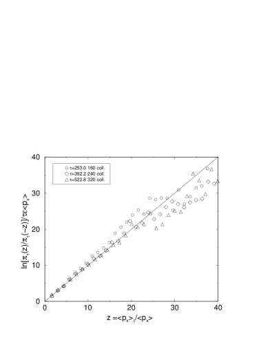
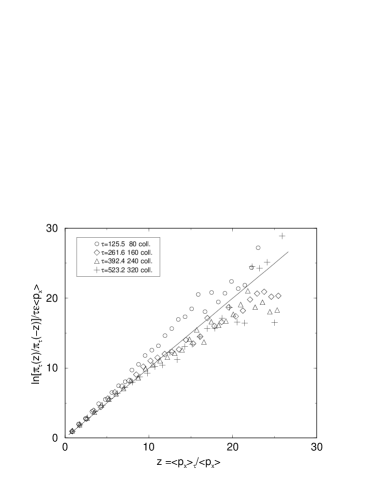
FIG. 5.: Test of the fluctuation relation for $\varepsilon=0.005$ (left) and $\varepsilon=0.01$ (right): the solid line is the theoretical prediction (5). Large $z$-values are more affected by statistical errors but its range of validity of it is larger for smaller field.

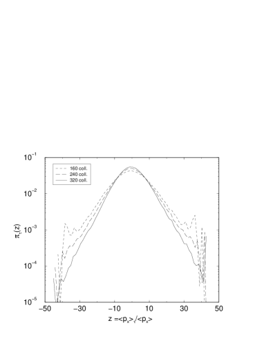
FIG. 6.: The distribution $\pi_{\tau}(z)$ of the fluctuation of the current for $\varepsilon=0.005$ (left) and $\varepsilon=0.01$ (right).

REFERENCES

- [1] D.J. Evans, E.G.D. Cohen and G.P. Morriss, Probability of second law violations in shearing steady flows, Phys. Rev. Lett. 71, 2401 (1993)
- [2] G. Gallavotti and E.G.D. Cohen, 1995, Dynamical ensembles in nonequilibrium statistical mechanics, Phys. Rev. Lett., 74, 2694. G. Gallavotti and E.G.D Cohen, 1995, Dynamical ensembles in stationary states, J. Stat. Phys., 80, 931
- [3] G. Gallavotti, 1996, Extension of Onsager’s reciprocity to large fields and the chaotic hypothesis, Phys. Rev. Lett. 78, 4334
- [4] G. Gallavotti, 1998, Chaotic dynamics, fluctuations, nonequilibrium ensembles, Chaos, 8(2) 384
- [5] F. Bonetto, G. Gallavotti, P. Garrido, 1997, Chaotic principle: an experimental test, Physica D, 105, 226
- [6] S. Ciliberto and C. Laroche, 1998, An experimental test of the Gallavotti-Cohen fluctuation theorem, Journal de Physique IV, vol 8 Pr6, 215
- [7] S. Lepri, R. Livi, A. Politi, 1998, Energy transport in anharmonic lattices close to and far from equilibrium, Physica D 119, 140
- [8] F. Bonetto, N. Chernov and J.L. Lebowitz, 1998, (Global and Local) Fluctuations of Phase Space Contraction in Deterministic Stationary Non-equilibrium, chao-dyn/9804020
- [9] L. Rondoni and E. Segre, 1998, Fluctuations in 2D reversibly-damped turbulence, chao-dyn/9810028
- [10] G. Gallavotti, 1997, Dynamical ensembles equivalence in fluid mechanics, Physica D, 105, 163
- [11] F. Bonetto and G. Gallavotti, 1997, Reversibility, coarse graining and the chaoticity principle, Comm. Math. Phys., 189, 263
- [12] C. Maes, 1998, The fluctuation theorem a a Gibbs property, archived in
- [13] J.L. Lebowitz and H. Spohn, 1998, A Gallavotti-Cohen type symmetry in the large deviation functional for Stochastic Dynamics, preprint, Rutgers University
- [14] J.L. Lebowitz, 1993, Boltzmann’s entropy and time’s arrow, Physics Today, September 1993, 38
- [15] J. Bricmont, 1997, Science of chaos or chaos in science?, Proc. New York Academy of Science (appendix 1. in particular)
- [16] E.G.D. Cohen and L. Rondoni, 1998, Note on phase space contraction and entropy production in thermostatted hamiltonian systems, Chaos, 8(2) 357
- [17] G. Benettin, P. Hjorth and P. Sempio, 1998, Exponentially long equilibrium times in a one dimensional collisional model of classical gas, preprint
- [18] C.P. Dettmann, E.G.D. Cohen, and H. van Beijeren, 1999, Microscopic chaos from Brownian motion?, xxx.lanl.gov/chao-dyn/99040041
- [19] D.J. Searles and D.J. Evans, 1994, Equilibrium microstates which generate second law violating steady states, Phys. Rev. E, 50, 1645
- [20] E.G.D. Cohen and G. Gallavotti, 1999, Note on two theorems in nonequilibrium statistical mechanics, xxx.lanl.gov/cond-mat/9903418
- [21] P. Gaspard et al. 1998, , Nature 394, 865
- [22] G. Gutkin, 1996, Billiards in polygons: Survey of recent results J. Stat. Phys. 83, 7
- [23] R. Artuso, 1997, Correlations and spectra of triangular billiards, Physica D, 109, 1
- [24] J. Lloyd, M. Niemeyer, L. Rondoni and G.P. Morriss, 1995, The nonequilibrium Lorentz gas, Chaos 5 (3) 536