The Radiative Kicked Oscillator: A Stochastic Web or Chaotic Attractor ?

Abstract

A relativistic charged particle moving in a uniform magnetic field and kicked by an electric field is considered. Under the assumption of small magnetic field, an iterative map is developed. We consider both the case in which no radiation is assumed and the radiative case, using the Lorentz-Dirac equation to describe the motion. Comparison between the non-radiative case and the radiative case shows that in both cases one can observe a stochastic web structure for weak magnetic fields, and, although there are global differences in the result of the map, that both cases are qualitatively similar in their small scale behavior. We also develop an iterative map for strong magnetic fields. In that case the web structure no longer exists; it is replaced by a rich chaotic behavior. It is shown that the particle does not diffuse to infinite energy; it is limited by the boundaries of an attractor (the boundaries are generally much smaller than light velocity). Bifurcation occurs, converging rapidly to Feigenbaum’s universal constant. The chaotic behavior appears to be robust. For intermediate magnetic fields, it is more difficult to observe the web structure, and the influence of the unstable fixed point is weaker.

]

I Introduction

Zaslavskii et al [3] studied the behavior of particles in the wave packet of an electric field in the presence of a static magnetic field. For a broad wave packet with sufficiently uniform spectrum, one may show that the problem can be stated in terms of an electrically kicked harmonic oscillator. For rational ratios between the frequency of the kicking field and the Larmor frequency associated with the magnetic field the phase space of the system is covered by a mesh of finite thickness; inside the filaments of the mesh, the dynamics of the particle is stochastic and outside (in the cells of stability), the dynamics is regular. This structure is called a stochastic web. It was found that this pattern covers the entire phase plane, permitting the particle to diffuse arbitrarily far into the region of high energies (a process analogous to Arnol’d diffusion [4]).

Since the stochastic web leads to unbounded energies, several authors have considered the corresponding relativistic problem (for a work which can be related to the relativistic stochastic web see [5]). Longcope and Sudan [6] studied this system (in effectively $1\frac{1}{2}$ dimensions) and found that for initial conditions close to the origin of the phase space there is a stochastic web, which is bounded in energy, of a form quite similar, in the neighborhood of the origin, to the non-relativistic case treated by Zaslavskii et al. Karimabadi and Angelopoulos [7] studied the case of an obliquely propagating wave, and showed that under certain conditions, particles can be accelerated to unlimited energy through an Arnol’d diffusion in two dimensions. Since an accelerated charged particle radiates, it is important to study the radiative corrections to this motion. We shall use the Lorentz-Dirac equation to compute this effect.

We compute solutions to this equation for the case of the kicked oscillator. Under the restriction of weak magnetic field, at low velocities, the stochastic web found by Zaslavskii et al[3] occurs; the system diffuses in the stochastic region to unbounded energy, as found by Karimabadi and Angelopoulos[7]. The velocity of the particle is light speed limited by the dynamical equations, in particular, by the suppression of the action of the electric field at velocities approaching the velocity of light [8].

For the case of a strong magnetic field case (a case which can not be examined in laboratory) the stochastic web, which may occur in the weak magnetic field case, does not appear and is replaced by a rich chaotic behavior. In this regime, the particle does not accelerate to infinite energy; it limited by the boundary of the chaotic attractor.

II Model

In the present study we will consider a charged particle moving in a uniform magnetic field, and kicked by an electric field. The effect of relativity, as well as the radiation of the particle, will be considered. We restrict ourselves to the “on mass shell” constraint (keeping constant ${\dot{x}}^{\mu}{\dot{x}}_{\mu}=-c^{2}$).

The fundamental equation that we use to study radiation is the Lorentz-Dirac equation [10],

$$m_{0}\ddot{x}^{\mu}={e\over c}\dot{x}_{\nu}F^{\mu\nu}+\gamma_{0}m_{0}({\stackrel{{\scriptstyle\dots}}{{x}}^{\mu}}-{1\over c^{2}}\dot{x}^{\mu}\ddot{x}_{\nu}\ddot{x}^{\nu}),$$ (1)

where $\gamma_{0}={2\over 3}{r_{0}\over c}=6.26\times 10^{-24}\sec$. The indices $\mu$ and $\nu$ indicate the coordinates $t$, $x$, $y$, and $z$ (or 0, 1, 2, 3), and the derivative is with respect to $\tau$, which can be regarded as proper time in the “on-mass-shell” case. $F^{\mu\nu}$ is the antisymmetric electromagnetic tensor. The first term of the right hand side of Eq. (1) is the relativistic Lorentz force, and the second term is the radiation-reaction term. Note that the small size of the radiation coefficient ($\gamma_{0}\ll 1$) leads to a singular equation that requires special mathematical treatment, as well as physical restrictions, as will be discussed in the succeeding sections.

Following Zaslavskii et al [3], the magnetic field is chosen to be uniform in the $z$ direction, and the kicking electric field is a function of $x$ in the $x$ direction,

$${\bf B} = (0,0,B)$$ (2)

$${\bf E}(x,t) = ({f(x){\sum_{n=-\infty}^{\infty}\delta(t-nT)}},0,0).$$ (3)

Originally, Zaslavskii et al chose a uniform broad band electric field wave packet which can be expanded as an infinite sum of (kicking) $\delta$-functions ($\omega_{0}$ is the frequency of the central harmonic of the wave packet, $k_{0}$ is the wave number of the central harmonic, and $\Delta\omega$ is the frequency between the harmonics of the wave packet)

$$E_{x}=E(x,t)=-E_{0}\sum_{n=-\infty}^{\infty}\sin(k_{0}x-\omega_{0}t-n\Delta\omega t),$$ (4)

which, for $\omega_{0}=0$, becomes

$$E(x,t)=-E_{0}T\sin(k_{0}x)\sum_{n=-\infty}^{\infty}\delta(t-nT),$$ (5)

where $T={{2\pi}\over{\Delta\omega}}$. Eq. (2) is the generalization of Eq. (5), with an arbitrary function $f(x)$ instead of the sine function of Eq. (5).

In order to introduce a map which connects between cycles of integration which start before a kick and end before the next electric field kick, one has first to integrate over the $\delta$ electric kick and then to integrate the equations of motion between the kicks, where only a uniform magnetic field is present and there is no electric field up to the beginning of the next kick.

III The motion of a charged particle in a uniform magnetic field

A An integration with respect to the proper time $\tau$

In the case of a uniform magnetic field in Eq. (2), Eqs. (1) reduce to three coupled differential equations,

$$c\ddot{t} =\ddot{x}_{0}= \gamma_{0}({\stackrel{{\scriptstyle\dots}}{{x}}_{0}}-{1\over{c^{2}}}\dot{x}_{0}R)$$ (6)

$$\ddot{x} =\ddot{x}_{1}= -\Omega\dot{x}_{2}+\gamma_{0}({\stackrel{{\scriptstyle\dots}}{{x}}_{1}}-{1\over{c^{2}}}\dot{x}_{1}R)$$ (7)

$$\ddot{y} =\ddot{x}_{2}= \Omega\dot{x}_{1}+\gamma_{0}({\stackrel{{\scriptstyle\dots}}{{x}}_{2}}-{1\over{c^{2}}}\dot{x}_{2}R),$$ (8)

where $\Omega={{e_{0}B_{0}}\over{m_{0}c}}$, $R=\ddot{x}_{1}^{2}+\ddot{x}_{2}^{2}-\ddot{x}_{0}^{2}$, and $e_{0}=-e$ (charge of the electron).

Using a complex coordinate[11], $u=x+iy$, Eqs. (6) can be written as,

$$\ddot{t} = \gamma_{0}({\stackrel{{\scriptstyle\dots}}{{t}}}-{1\over{c^{2}}}\dot{t}R)$$ (9)

$$\ddot{u} = i\Omega\dot{u}+\gamma_{0}({\stackrel{{\scriptstyle\dots}}{{u}}}-{1\over{c^{2}}}\dot{u}R).$$ (10)

It is very convenient to use the hyperbolic coordinates,

$$\dot{t} = \cosh q$$ (11)

$$\dot{x} = c\sinh q\cos\phi$$ (12)

$$\dot{y} = c\sinh q\sin\phi$$ (13)

since the constraint (see [9] for further discussion),

$$\dot{x}^{\mu}\dot{x}_{\mu}=\dot{x}^{2}+\dot{y}^{2}-c^{2}\dot{t}^{2}=-c^{2},$$ (14)

is then automatically satisfied. The complex coordinate $u$ then becomes,

$$\dot{u}=c\sinh qe^{i\phi}$$ (15)

and the equations of motion Eqs. (9) can be written as,

$$\dot{q} = -\gamma_{0}\dot{\phi}^{2}\cosh q\sinh q+\gamma_{0}\ddot{q}$$ (16)

$$\dot{\phi} = \Omega+2\gamma_{0}\dot{\phi}\dot{q}\coth q+\gamma_{0}\ddot{\phi}.$$ (17)

As pointed out earlier, in the case of a singular equation (such as Eqs. (16) and (17)), one has to consider physical arguments as well as mathematical arguments. There are several suggested methods to avoid the “run away electron” problem [10]. One of the most frequently used, especially useful for scattering problems, assumes [12] that the particle loses all its energy after a sufficiently large time, and the run away parts of the solution are set to zero; the equations of motion can then be written as an integral equation. Another method, which permits the study of problems with only non-asymptotic states [13], uses an iterative singular perturbation integration that leads to the stable solution. Since the integration we must use is over a finite time, it is impossible to use an asymptotic condition (e.g. $|v|\to 0$ at $\tau\to\infty$). The approach of Sokolov and Ternov [11] is more suitable for our purpose, since it can be implemented for bounded time integration, and the mathematical solution is simple. In this method, in the first step, the perturbation terms in Eq. (17) are disregarded (as in the iterative scheme of [13]), and then the resulting equation is exactly integrated. In the second step, the singular term on the right hand side of Eq. (16) is not considered; using $\phi(\tau)$ from Eq. (17), the equation including just the first term is integrated. The solution is [11]

$$\phi = \Omega\tau$$ (18)

$$\beta(\tau) = \tanh q={v_{0}\over c}e^{-\gamma_{0}\Omega^{2}\tau}=\beta_{0}e^{-{\tau\over\tau_{0}}},$$ (19)

where $\beta_{0}={v_{0}\over c}$ is the actual initial velocity divided by $c$, and $\tau_{0}={1\over{\gamma_{0}\Omega^{2}}}$ is the decay time for the energy of the particle.

To get an estimate for the radiation during one cycle, consider the maximal uniform magnetic field that can achieved today in a laboratory, which is ${\cal O}(10T)={\cal O}(10^{5}\,{\rm gauss})$. If, for example, $B_{0}=10^{5}\,{\rm gauss}$, then $\Omega=1.76\times 10^{12}{1\over\sec}$, and $\tau_{0}=5\times 10^{-2}\sec$. Thus, it is clear from Eq. (18) that the particle makes ${\Omega\over{2\pi}}\tau_{0}\approx 10^{10}$ cycles before it decays to ${1\over e}$ of its initial velocity. In other words, the energy loss during one cycle in very small, and since in our problem, the time $T$ between the kicking is of the order of the period, the energy loss between consecutive kicks is very small.

The time between the kicking is measured according to the observed time along the motion, $\Delta t=T$. Thus, it is necessary to find the corresponding $\Delta\tau$. It follows from Eq. (11) and Eq. (18) that,

$$\dot{t}=\cosh q={1\over\sqrt{1-\beta^{2}_{0}e^{-{{2\tau}\over{\tau_{0}}}}}}.$$ (20)

The solution of Eq. (20) can be obtained by a elementary integration,

$$t=\tau_{0}\ln\left({{1+\sqrt{1-a^{2}}}\over a}C_{1}\right),$$ (21)

where $a=\beta_{0}e^{-{\tau\over{\tau_{0}}}}$. After some algebra one gets,

$$\Delta\tau=\tau_{0}\ln\left({1\over 2}{{\beta_{0}^{2}+(1+\sqrt{1-\beta_{0}^{2}})^{2}e^{2T/\tau_{0}}}\over{(1+\sqrt{1-\beta_{0}^{2}})e^{T/\tau_{0}}}}\right).$$ (22)

In Fig. 1 we present the behavior of the function ${{\Delta\tau(T/\tau_{0})}\over{\tau_{0}}}$. It can be seen from Fig. 1 that in any case,

$$\Delta\tau\leq T;$$ (23)

this implies that the time difference according to the proper time $\tau$ is always less then the time difference according to observed time $t$. This fact is corresponds to the well known relativistic “time-dilation” phenomenon. The inequality Eq. (23) can be also illustrated by considering the two extreme cases,

$$T\ll\tau_{0} \Rightarrow \Delta\tau\approx T\sqrt{1-\beta_{0}^{2}}+{{\beta_{0}^{2}}\over 2}{{T^{2}}\over{\tau_{0}}}+{\cal O}(T^{3})$$ (24)

$$T\gg\tau_{0} \Rightarrow \Delta\tau\approx T+\tau_{0}\ln\left({{1+\sqrt{1-\beta_{0}^{2}}}\over 2}\right).$$ (25)

For strong magnetic field (i.e. the case of Eq. (25)) the numerator is less than (or equal) to 2 and thus the $ln$ function will give a negative number; in this case the inequality Eq. (23) is clearly achieved. For a low magnetic field Eq. (24) behaves like a parabola; the slope at $T=0$ is $\sqrt{1-\beta_{0}^{2}}$ which is less than one, and thus the inequality Eq. (23) is satisfied. In the present study we will consider separately the cases of weak magnetic field (Eq. (24) and strong magnetic field (Eq. (25)).

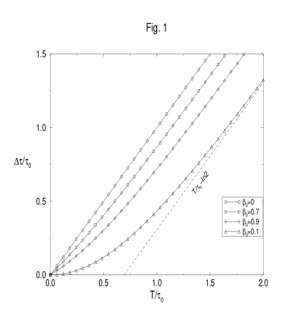
FIG. 1.: The function ${{\Delta\tau(T/\tau_{0})}\over{\tau_{0}}}$ versus $T/\tau_{0}$. Four typical cases are shown ($\beta_{0}=0$, $\beta_{0}=0.7$, $\beta_{0}=0.9$, $\beta_{0}=1$). All possible curve lines between the graphs of $\beta_{0}=0$ and $\beta_{0}=1$. The dashed line indicates the asymptotic behavior of the case $\beta_{0}=1$.

B An integration with respect to the observed time $t$

In the previous subsection we have shown the approximate solution for a charged particle moving in a uniform magnetic field. However, as mentioned above, the kicking of the electric field from Eq. (2) is with respect to the observed time $t$, and it is therefore convenient to integrate the equations of motion (Eqs. (16) and (17)) with respect to $t$.

The arguments that were used in order to obtain Eqs. (18), as well as the implementation of the chain rule on Eqs. (16) and (17) by the use of Eq. (11), lead to the following equations of motion

$${{dq}\over{dt}} = -{1\over{\tau_{0}}}\sinh q$$ (26)

$${{d\phi}\over{dt}} = {\Omega\over{\cosh q}}.$$ (27)

A simple integration of Eq. (26) yields,

$$\tanh{q\over 2}=e^{C_{1}}e^{-{t\over{\tau_{0}}}},$$ (28)

where $C_{1}<0$. Substitution of Eq. (28) in Eq. (27) gives,

$${{d\phi}\over{dt}}=\Omega\tanh({t\over{\tau_{0}}}-C_{1}),$$ (29)

and the solution is

$$\phi=\Omega\tau_{0}\ln\cosh({t\over{\tau}}-C_{1})+C_{2},$$ (30)

where $C_{1}=\cosh^{-1}({1\over{\beta_{0}}})$, and $C_{2}=\tan^{-1}(\dot{y}_{0}/\dot{x}_{0})+\Omega\tau_{0}\ln\beta_{0}$. Returning to the original $x$, $y$ coordinates (using Eqs. (11)), the equations of motion become,

$${{dx}\over{dt}} = c{{\cos(\Omega\tau_{0}\ln(\cosh(t/\tau_{0}-C_{1}))+C_{2})}\over{\cosh(t/\tau_{0}-C_{1})}}$$ (31)

$${{dy}\over{dt}} = c{{\sin(\Omega\tau_{0}\ln(\cosh(t/\tau_{0}-C_{1}))+C_{2})}\over{\cosh(t/\tau_{0}-C_{1})}}.$$ (32)

It is possible to write Eq. (32) in more convenient way, by using the relation

$$\cosh({t\over{\tau_{0}}}-C_{1})={1\over{\beta_{0}}}\cosh{t\over{\tau_{0}}}+{1\over{\beta_{0}}}\sqrt{1-\beta_{0}^{2}}\sinh{t\over{\tau_{0}}}.$$ (33)

Eqs. (32) then become

$${{dx}\over{dt}} = {{\left({{dx}\over{dt}}\right)_{0}\cos\alpha-\left({{dy}\over{dt}}\right)_{0}\sin\alpha}\over{\cosh{t\over{\tau_{0}}}+\sqrt{1-\beta_{0}^{2}}\sinh{t\over{\tau_{0}}}}}$$ (34)

$${{dy}\over{dt}} = {{\left({{dx}\over{dt}}\right)_{0}\sin\alpha+\left({{dy}\over{dt}}\right)_{0}\cos\alpha}\over{\cosh{t\over{\tau_{0}}}+\sqrt{1-\beta_{0}^{2}}\sinh{t\over{\tau_{0}}}}},$$ (35)

where

$$\alpha=\Omega\tau_{0}\ln(\cosh{t\over{\tau_{0}}}(1+\sqrt{1-\beta_{0}^{2}}\tanh{t\over{\tau_{0}}})).$$ (36)

It is necessary to integrate Eq. (35) since the value of $x$ is used in the electric field kicking in Eq. (2). There is no analytical solution to Eq. (35), and a numerical integration must, in general, be performed. In the succeeding sections we will study separately the case of weak magnetic field (i.e. $T/\tau_{0}\ll 1$) and the case of strong magnetic field (i.e. $T/\tau_{0}\gg 1$).

IV Derivation of the map - weak magnetic field

A The approximated solution for the weak magnetic field case

When dealing with weak magnetic field we restrict ourselves to $T/\tau_{0}\ll 1$, and it is possible to expand ${{dx}\over{dt}}$ and ${{dy}\over{dt}}$ in a Taylor series and then to integrate. The expansion of Eq. (36) is

$$\alpha\approx\Omega\sqrt{1-\beta_{0}^{2}}t+{1\over 2}\beta_{0}^{2}{{t^{2}}\over{\tau_{0}}}+{1\over 3}\sqrt{1-\beta_{0}^{2}}{{t^{3}}\over{\tau_{0}^{2}}}({3\over 2}-\beta_{0}^{2})+{\cal O}({{{t^{4}}\over{\tau_{0}^{3}}}}).$$ (37)

The first order expansion (according to $t/\tau_{0}$) of Eqs. (35) is

$${{dx}\over{dt}}={1\over{1+{1\over\gamma}{t\over{\tau_{0}}}}} \left[\left({{dx}\over{dt}}\right)_{0}\cos({{\Omega}\over\gamma}t+{1\over 2}\Omega\beta_{0}^{2}{{t^{2}}\over{\tau_{0}}})\right.$$ (39)

$$\left.-\left({{dy}\over{dt}}\right)_{0}\sin({{\Omega}\over\gamma}t+{1\over 2}\Omega\beta_{0}^{2}{{t^{2}}\over{\tau_{0}}})\right]$$

$${{dy}\over{dt}}={1\over{1+{1\over\gamma}{t\over{\tau_{0}}}}} \left[\left({{dx}\over{dt}}\right)_{0}\sin({{\Omega}\over\gamma}t+{1\over 2}\Omega\beta_{0}^{2}{{t^{2}}\over{\tau_{0}}})\right.$$ (41)

$$\left.+\left({{dy}\over{dt}}\right)_{0}\cos({{\Omega}\over\gamma}t+{1\over 2}\Omega\beta_{0}^{2}{{t^{2}}\over{\tau_{0}}})\right],$$

where $\gamma=1/\sqrt{1-\beta_{0}^{2}}$. Since ${1\over\gamma}{t\over{\tau_{0}}}\ll 1$, one can use the approximation,

$${1\over{1+{1\over\gamma}{t\over{\tau_{0}}}}}\approx{{1-{1\over\gamma}{t\over{\tau_{0}}}}}.$$ (42)

Using Eq. (42), the actual velocities, $dx/dt$ and $dy/dt$, from Eq. (41) can be integrated and expressed by elementary Fresnel functions. However, the effect of radiation is due to the ${1\over\gamma}{t\over{\tau_{0}}}$ term (which multiplies the sine and cosine functions), and the ${1\over 2}\Omega\beta_{0}^{2}{{t^{2}}\over{\tau_{0}}}$ term is not essential since the major offset from the unstable fixed point is due to the ${{\Omega}\over\gamma}t$ term.

Under the above assumptions the resulting equations are,

$$\left({{dx}\over{dt}}\right)_{T} = \left(1-{T\over{\gamma\tau_{0}}}\right)\times$$ (44)

$$\left[\left({{dx}\over{dt}}\right)_{0}\cos({{\Omega}\over\gamma}T)-\left({{dy}\over{dt}}\right)_{0}\sin({{\Omega}\over\gamma}T)\right]$$

$$\left({{dy}\over{dt}}\right)_{T} = \left(1-{T\over{\gamma\tau_{0}}}\right)\times$$ (46)

$$\left[\left({{dx}\over{dt}}\right)_{0}\sin({{\Omega}\over\gamma}T)+\left({{dy}\over{dt}}\right)_{0}\cos({{\Omega}\over\gamma}T)\right].$$

One therefore obtains

$$x_{T}\approx{\gamma\over\Omega} \left[\left({{dy}\over{dt}}\right)_{T}-\left({{dy}\over{dt}}\right)_{0}\right]-$$ (48)

$${\gamma\over{\Omega^{2}\tau_{0}}}\left[\left({{dx}\over{dt}}\right)_{T}-\left({{dx}\over{dt}}\right)_{0}\right]+x_{0}.$$

The exponential decay from Eqs. (32) is replaced by linear decay; by squaring Eq. (44) and Eq. (46) one obtains the linear relation $v(T)=\sqrt{v_{x}^{2}+v_{y}^{2}}=v_{0}(1-T/\gamma\tau_{0})$.

B Integration over a $\delta$ electric kick

As pointed out in the previous section, the Lorentz-Dirac equation (Eq. (1)) is a singular equation. The electric field which is used in this paper was expanded to a sum of $\delta$ functions (Eq. (2)). In that case, Eq. (1) can not be integrated over the kick by regular treatment, and some approximation for the $\delta$ function should be considered instead. However, since the radiation has its effect in the direction of the relevant coordinate (in our case it is the $x^{1}=x$ coordinate), and because of the infinitesimal time interval, it is possible to replace the kicking parameter, $K$, by an effective kicking strength, which should be a smaller number than the original one. Thus, the nature of the solution for the system will not change due to the radiation during the kicking. The constant magnetic field during the kick is not considered since the integration is over an infinitesimal time interval.

Under the above assumptions, in the neighborhood of the kick, the Lorentz-Dirac equation, Eq. (1), can be written as,

$${d\over{dt}}\left({{dx}\over{d\tau}}\right) = {f(x){\sum_{n=-\infty}^{\infty}\delta(t-nT)}}$$ (49)

$${d\over{dt}}\left({{dy}\over{d\tau}}\right) = 0.$$ (50)

Integration over the $\delta$ function yields,

$$\left({{dx}\over{d\tau}}\right)_{+} = \left({{dx}\over{d\tau}}\right)_{-}+f(x)$$ (51)

$$\left({{dy}\over{d\tau}}\right)_{+} = \left({{dy}\over{d\tau}}\right)_{-}$$ (52)

where the + sign indicates after the kick, and the - sign, before the kick. Following Ref. [3], we choose,

$$f(x)={{eET}\over{m_{0}}}\sin\,kx=K\sin\,kx.$$ (53)

Using the fact that ${d\over{d\tau}}=\gamma{d\over{dt}}$ one obtains the following relations,

$$\gamma_{+} = \sqrt{1+{1\over{c^{2}}}\left[\left(\gamma_{-}\left({{dx}\over{dt}}\right)_{-}+f(x_{n})\right)^{2}+\gamma_{-}^{2}\left({{dy}\over{dt}}\right)_{-}^{2}\right]}$$ (56)

$$\left({{dx}\over{dt}}\right)_{+}={\gamma_{-}\over\gamma_{+}}\left({{dx}\over{dt}}\right)_{-}+{1\over\gamma_{+}}f(x_{n})$$

$$\left({{dy}\over{dt}}\right)_{+}={\gamma_{-}\over\gamma_{+}}\left({{dy}\over{dt}}\right)_{-}.$$

Returning to the initial charge $e=-e_{0}$ and thus $\Omega\to-\Omega$, the map which connects the velocities from just before the kick to the next kick (by the use of Eqs. (44)-(48)) is,

$$\left({{dx}\over{dt}}\right)_{n+1} =\left(1-{T\over{\gamma_{+}\tau_{0}}}\right)\times$$ (58)

$$\left[\left({{dx}\over{dt}}\right)_{+}\cos({{\Omega}\over{\gamma_{+}}}T)+\left({{dy}\over{dt}}\right)_{+}\sin({{\Omega}\over{\gamma_{+}}}T)\right]$$

$$\left({{dy}\over{dt}}\right)_{n+1} =\left(1-{T\over{\gamma_{+}\tau_{0}}}\right)\times$$ (60)

$$\left[-\left({{dx}\over{dt}}\right)_{+}\sin({{\Omega}\over{\gamma_{+}}}T)+\left({{dy}\over{dt}}\right)_{+}\cos({{\Omega}\over{\gamma_{+}}}T)\right]$$

$$x_{n+1} \approx-{{\gamma_{+}}\over\Omega}\left[\left({{dy}\over{dt}}\right)_{n+1}-\left({{dy}\over{dt}}\right)_{+}\right]$$ (62)

$$-{{\gamma_{+}}\over{\Omega^{2}\tau_{0}}}\left[\left({{dx}\over{dt}}\right)_{n+1}-\left({{dx}\over{dt}}\right)_{+}\right]+x_{n}.$$

Notice that the minus signs in Eq. (56) refer to the $n^{th}$ points of the map.

It is possible to return to the non-radiative limit by letting ${1\over{\tau_{0}}}\to 0$. In that case the map is equivalent to the map which was derived by Longcope and Sudan [6]. The nonrelativistic limit, which was derived by Zaslavskii et al [3], is achieved by letting ${1\over{\tau_{0}}}\to 0$ and $c\to\infty$.

C Analysis

Up to the derivation of Eqs. (58)-(62) we have passed three stages, (a) the velocities were calculated using an exact solution and the position $x$ can be calculated by numerical integration (Eqs. (35)), (b) the velocities were approximated by Eqs. (41) and the position $x$ by the elementary Fresnel function, and (c) the velocities were approximated by Eqs. (58)-(60) and the position $x$ (Eq. (62)) was derived using elementary integration. Among all the combinations of the solutions for the velocities and the position $x$ we choose the combination of the exact solution of velocities (case (a), Eqs. (35)) and the exact solution for the position $x$ (stage (c), Eq. (62)). The value of $x$ was selected from the third stage of our derivation since it enters the equation just in the kicking term, and there it affects only slightly the phase. Thus, one does not expect that this fact can change the typical behavior of the particle. The above analysis is summarized in Fig. 2.

FIG. 2.: A diagram which present the all possibilities for the map construction. The wider line indicates the chosen combination.

The radiative map is then

$$\left({{dx}\over{dt}}\right)_{n+1} = {{\left({{dx}\over{dt}}\right)_{+}\cos\alpha+\left({{dy}\over{dt}}\right)_{+}\sin\alpha}\over{\cosh{t\over{\tau_{0}}}+\sqrt{1-\beta_{+}^{2}}\sinh{t\over{\tau_{0}}}}}$$ (63)

$$\left({{dy}\over{dt}}\right)_{n+1} = {{-\left({{dx}\over{dt}}\right)_{+}\sin\alpha+\left({{dy}\over{dt}}\right)_{+}\cos\alpha}\over{\cosh{t\over{\tau_{0}}}+\sqrt{1-\beta_{+}^{2}}\sinh{t\over{\tau_{0}}}}}$$ (64)

$$x_{n+1} = -{{\gamma_{+}}\over\Omega}\left[\left({{dy}\over{dt}}\right)_{n+1}-\left({{dy}\over{dt}}\right)_{+}\right]$$ (66)

$$-{{\gamma_{+}}\over{\Omega^{2}\tau_{0}}}\left[\left({{dx}\over{dt}}\right)_{n+1}-\left({{dx}\over{dt}}\right)_{+}\right]+x_{n},$$

where the values immediately after the kick are as in Eqs. (56) and $\alpha$ is defined in Eq. (36) ($\alpha\to-\alpha$ since $e=-e_{0}$) . Note that for our limit ($T/\tau_{0}\ll 1$) there is not a great difference between the map given by Eqs. (58)-(62) and Eqs. (63)-(66).

V Results - weak magnetic field

In order to obtain a web structure, there are two conditions that have to be fulfilled. In the nonrelativistic case, the first condition is that the ratio between the gyration frequency, $\Omega$, and the kicking time, $T$, is a rational number, a condition which can be expressed as follows,

$$\Omega T=2\pi{p\over q}$$ (67)

where $p$, and $q$, are integer numbers. Secondly, one must start from the neighborhood of the unstable fixed point (otherwise, the particle will not diffuse, and will not create a web structure),

$$\left({{dx}\over{dt}}\right)_{0} = 0$$ (68)

$$\left({{dy}\over{dt}}\right)_{0} \cong (2n+1){{\pi\Omega}\over k},$$ (69)

where $n$ is an integer number. The symmetry of the web is determined by $p$ and $q$. If, for example $p=1$ and $q=4$, the particle is kicked four times during one cycle, and thus, the symmetry of the web will be a four symmetry [3].

In the relativistic case [6], the above conditions are slightly different, because of the additional factor $\sqrt{1-\beta_{0}^{2}}$ which multiplies the $\Omega T$ term. However, if the initial velocities are small, i.e. $v_{0}\ll c$, the additional factor is close to 1, and thus the structure of the web should not change. In the radiative and relativistic case, as well as the non-radiative relativistic case, conditions (67) and (69) become,

$$\left({{dx}\over{dt}}\right)_{0} = 0$$ (70)

$$\left({{dy}\over{dt}}\right)_{0} \cong (2n+1)\sqrt{1-\beta_{0}^{2}}{{\pi\Omega}\over k}.$$ (71)

For sufficiently large initial velocities the above conditions do not hold anymore, and the web structure is not observed.

In this section we will compare (qualitatively; a quantitative treatment for the diffusion rate will be studied elsewhere) the diffusion of the non-radiative particle and the radiative particle. Intuitively, one would expect that a radiative particle will diffuse more slowly than a non-radiative one, since the radiation effects act like friction, and are thus expected to “stop” the particle. However, this naive expectation is not true, as we will demonstrate below.

In order to investigate the above assumption, we have chosen a four symmetry structure ($q=4$). We used the same initial conditions for all cases; just the kicking strength $K$ has been changed. The parameters values and the initial conditions were $B=10$, $v_{x,0}=0$, $v_{y,0}=4\times 10^{-5}$, $k=10$, and the number of iterations was $N=10^{6}$. In Fig. 3, we present the results as follows: the first column is the non-radiative case, the second column is the radiative case, and the third column is the total velocity versus the iteration number (the circles indicates the non-radiative case and the squares the radiative one). In the first row $K=1\times 10^{-5}$, in the second $K=2\times 10^{-5}$, and in the third $K=4\times 10^{-5}$.

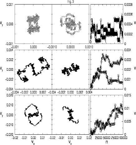
FIG. 3.: Different types of diffusion behavior as described in the context.

As can be seen clearly from Fig. 3, the web structure is valid for the radiative case (top panel, second column). The web structure is also exists in the other cases; the web cells are very small and they are difficult to see. Although the radiative particle and the non-radiative particle start from the same initial conditions they behave differently.

In some cases the diffusion rate of the radiative case is larger than the diffusion rate of the non-radiative case, for example, in the top and the bottom panels after $9\times 10^{5}$ iterations the radiative particle reaches a higher velocity than the non-radiative one. On the other hand, in the middle panel the radiative particle is slower then non-radiative one. Obviously, it is impossible to draw any general conclusion for the question of whether a non-radiative particle is faster then the radiative one. For this a more systematic approach should be carried out. This would be beyond the scope of the present paper and will be considered elsewhere.

When the velocity of the particle reaches close to the velocity of light it actually stops growing (according to evolution in the time $t$) although it increases its energy. In Fig. 4 we show an example for that behavior. The parameters values are : $B=10$, $v_{x,0}=0$, $v_{y,0}=1\times 10^{-5}$, $k=10$, $K=0.01$, and the number of iterations was $N=1\times 10^{6}$ (every $10^{\rm th}$ iteration was plotted). Fig. 4a and Fig. 4c are the non-radiative cases, while Fig. 4b and Fig. 4d are the radiative cases; in Fig. 4a and Fig. 4b the map of $v_{x}$ versus $v_{y}$ is presented, while in Fig. 4c and Fig. 4d the total velocity $v$ versus the iteration number is plotted (every $10^{\it th}$ iteration was plotted). As seen from Fig. 4, the particle accelerates quickly to high velocity, and most of the time stays with this high velocity, approaching light velocity asymptotically, while increasing its energy to infinity.

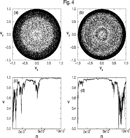
FIG. 4.: The behavior of a particle with high velocity. (a) the non-radiative map, (b) the radiative map, (c) the total velocity of the non-radiative case, and (d) the total velocity of the radiative case.

VI Derivation of the map - strong magnetic field

A Introductory remarks

In the preceding section we discussed the realistic case of weak magnetic field. In this section we will consider the other limit, i.e., the strong magnetic field limit. Despite of the difficulties in producing a strong, uniform, and stable magnetic field, one can assume that such fields do exist near astronomical objects, such as, neutron stars.

When increasing the magnetic field strength the radiation effects become more dominant; for strong enough magnetic field the particle loses most of its energy before the next kicking. Then, the kick of the electric field “pump” energy into the particle, which again radiate most of this energy before the next kick. Obviously, if the kicking strength, $K$, is small, the particle will lose its energy in an exponential way, and will spiral in to zero velocity (in the velocity phase space). On the other hand, if $K$ is strong enough, the energy gain due to the kicking is larger than energy loss due the radiation. In this case, the particle will increase its energy (not necessarily due to Arnol’d diffusion), and the velocity phase space will be limited.

The interesting phenomena occur when the energy loss due to the radiation is approximately equal to the pumping energy due to the kicking of the electric field. In that case one can expect that : a) the velocity of the particle will decrease to zero, b) the particle behavior (in the velocities phase space) is a chaotic behavior, c) the particle will diffusion (while increasing its velocity) through the web like structure, or d) the particle will increase its velocity in a stochastic way, not through a web like structure.

B The approximated solution for the strong magnetic field case

For strong magnetic field, we assume $T\gg\tau_{0}$. In this case, it is more convenient to write Eq. (33) as

$$\beta_{0}\cosh({t\over{\tau_{0}}}-C_{1})={1\over 2}e^{{t\over{\tau_{0}}}}\bigl{(}1+\sqrt{1-\beta_{0}^{2}}\bigr{)}\bigl{(}1+\xi^{2}\bigr{)},$$ (72)

where

$$\xi=e^{-{t\over{\tau_{0}}}}{\beta_{0}\over{1+\sqrt{1-\beta_{0}^{2}}}}.$$ (73)

Eq. (36) can be written as,

$$\alpha=\Omega t+\Omega\tau_{0}\ln\biggl{(}{{1+\sqrt{1-\beta_{0}^{2}}}\over 2}\biggr{)}+\Omega\tau_{0}\ln(1+\xi^{2}).$$ (74)

When $T\gg\tau_{0}$, $\xi\ll 1$ and in the first approximation, $\xi$ is negligible. Under those circumstances, Eqs. (35) become,

$${{dx}\over{dt}}= {2\over{1+\sqrt{1-\beta_{0}^{2}}}}e^{-{t\over{\tau_{0}}}}\times$$ (76)

$$\biggl{[}\biggl{(}{{dx}\over{dt}}\biggr{)}_{0}\cos(\Omega t+\phi_{0})-\biggl{(}{{dy}\over{dt}}\biggr{)}_{0}\sin(\Omega t+\phi_{0})\biggr{]}$$

$${{dy}\over{dt}}= {2\over{1+\sqrt{1-\beta_{0}^{2}}}}e^{-{t\over{\tau_{0}}}}\times$$ (78)

$$\biggl{[}\biggl{(}{{dx}\over{dt}}\biggr{)}_{0}\sin(\Omega t+\phi_{0})+\biggl{(}{{dy}\over{dt}}\biggr{)}_{0}\cos(\Omega t+\phi_{0})\biggr{]}$$

where

$$\phi_{0}=\Omega\tau_{0}\ln\biggl{(}{{1+\sqrt{1-\beta_{0}^{2}}}\over 2}\biggr{)}.$$ (79)

In the present case ($T\gg\tau_{0}$) $\phi_{0}\ll 0$, since $\Omega T\sim 1$ (see Eq. (67)).

Integration of Eq. (76) yields,

$$x(t)={{\tau_{0}}\over{1+\Omega^{2}\tau_{0}^{2}}}\biggl{[} -\biggl{(}{{dx}\over{dt}}\biggr{)}(t)+\biggl{(}{{dx}\over{dt}}\biggr{)}_{0}+$$ (81)

$$\Omega\tau_{0}\biggl{(}\biggl{(}{{dy}\over{dt}}\biggr{)}(t)-\biggl{(}{{dy}\over{dt}}\biggr{)}_{0}\biggr{)}\biggr{]}+x_{0}.$$

We now return to the initial charge $e=-e_{0}$ and thus change $\Omega\to-\Omega$ and $\alpha\to-\alpha$. The discussions from Sec. IV C are valid also here; Eqs. (63)-(64) remain the same and Eq. (66) should be replaced by

$$x_{n+1}=-{{\tau_{0}}\over{1+\Omega^{2}\tau_{0}^{2}}} \biggl{[}\biggl{(}{{dx}\over{dt}}\biggr{)}_{n+1}-\biggl{(}{{dx}\over{dt}}\biggr{)}_{+}+$$ (83)

$$\Omega\tau_{0}\biggl{(}\biggl{(}{{dy}\over{dt}}\biggr{)}_{n+1}-\biggl{(}{{dy}\over{dt}}\biggr{)}_{+}\biggr{)}\biggr{]}+x_{n}.$$

Note that since the velocities in Eq. (83) are limited by one, and since $\Omega\tau_{0}\ll 1$ and $\tau_{0}\ll 1$ the difference $x_{n+1}-x_{n}$ will be a very small number.

In order to observe some interesting behavior the effective kicking should be strong enough. The increments in the phase are very small number since $x_{n+1}-x_{n}={\cal O}(\tau_{0}v_{0})$ when $B\gg 1$. Thus, it is necessary to choose sufficiently large $k$ in the kicking function, $f(x_{n})=K\sin{kx_{n}}$ (Eqs. (53)-(56)),

$$k={\cal O}\bigg{(}{1\over{\tau_{0}v_{0}}}\bigg{)}.$$ (84)

In our calculations, we used

$$k={\pi\over{\tau_{0}v_{0}}}.$$ (85)

Obviously, the behavior also depends on the kicking strength, $K$. For small $kx$ the kicking approximated by $f(x)=K\sin\,kx\approx Kkx$. Thus, in some cases, large $K$ is equivalent to large $k$.

VII Results - strong magnetic field

In order to analyze the parameter space, one should first determine the most important parameters in the system. In our case the parameters are the kicking strength, $K$, and the magnetic field strength, $B$. The initial conditions, $v_{x,0}$, $v_{y,0}$, $x_{0}$, were chosen to be much smaller than the light velocity $c$, since in this regime the relativistic effects are negligible, and the radiation effects are isolated from the relativistic effects. However, in spite of those small initial conditions, one can easily determine what would happen if those initial conditions were in the order of the light velocity; for large enough kicking strength, $K$, the particle will accelerate to that regime.

Generally, a parameter space mapping requires a calculation of Lyapunov exponents [14, 15]. However, in our case, because of the decaying terms in Eqs. (63)-(64), we are interesting in the decaying regions. For this, the standard deviation,

$$\Delta v=\sqrt{<v^{2}>-<v>^{2}},$$ (86)

is considered (after a sufficiently large number of iterations when the motion converges to its stable behavior). In the case of decaying velocities, $v\to 0$, and thus, $\Delta v\to 0$. In the most cases of periodic motion $v={\rm const}$ and thus, $\Delta v=0$. As will be shown in the following, there exists a bifurcation behavior in the system, and since the gap between bifurcation points decreases exponentially, the period one region is much larger than the other periods (the exponential decrease start from the point between period one and period two, and do not include the period one itself). Moreover, since it is very difficult to balance the kicking strength, $K$, with the magnetic field strength, $B$, in such a way that the pumping energy due to the kick will be radiated before the next kick, just a small part of the parameter space will lead to a quasiperiodic or to a periodic motion. The dominant part of the parameter phase space should be either chaotic or stochastic, and thus should be indicated by a larger value of $\Delta v$. A high value of $\Delta v$ simply means that the basin of attraction (if it exists) is larger.

In Fig. 5a we present a density plot of the parameter phase space (the height is $\Delta v$). The darker regions have higher $\Delta v$. For small $K$ the velocity decays to zero. For larger $K$ the basin of attraction is larger, and one expect to find a more complex behavior. However, there exist stability lines which reflect that the particle either loses its energy or moves in a periodic motion. The stability lines seems to be continuous lines with well defined shape (the small discontinuities can be related to a high period level of the orbit; in this case $\Delta v\not\to 0$ but $\Delta v$ will be relatively small). Even for large $K$ values, in which the particle is kicked very strongly, it can move in a periodic way. However, those lines accumulate just a minor part of the parameter phase space, and thus one can expect to find a chaotic behavior near the neighborhood of an arbitrary point in parameter phase space [14]. Such a parameter phase space gives an indication of a robust chaotic system [15] with three positive Lyapunov exponents. Fig. 5b shows a contour plot of Fig. 5a.

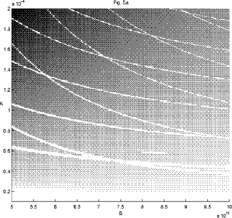
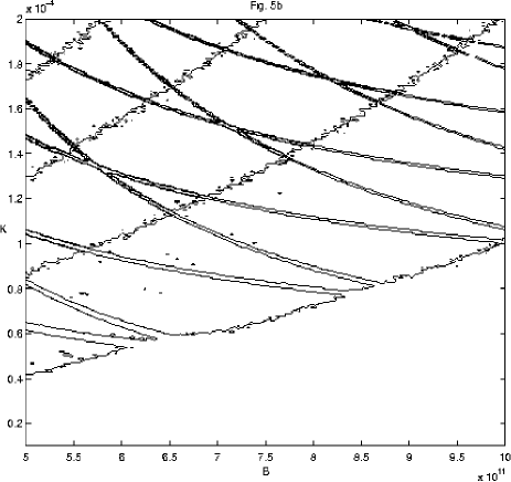
FIG. 5.: The parameter space, $B:K$, mapping. (a) A density plot of the parameter space. The darker regions indicate high velocity standard deviation. (b) Contour plot of (a).

Taking the a fixed magnetic field value, B, and changing the kicking strength, $K$, will give more inset about the particle behavior. In Fig. 6a we have plotted a bifurcation map using $K$ as the relevant parameter. For each $K$ value we have iterate the map for several thousand of iterations and plotted just the last few hundred of points (this have done to make sure that the particle was convergent to its basin of attraction). For small $K$ values, the particle do not kicked strong enough, and it loses its energy exponentially to zero. For higher $K$ values ($K=1.35\times 10^{-5}-2.25\times 10^{-5}$) the particle has a constant velocity. Then, a series of bifurcation points appears, leading to the chaotic region (the enlargement of the solid rectangle is shown in the inset, where the bifurcation points can be clearly seen). The chaotic region which follows afterwards ends with other period one points, followed by another set of bifurcation points, and so on. The regular regions of Fig. 6a are parts of the stability line of Fig. 5. The maximum velocity that the particle reaches seems to grow linearly.

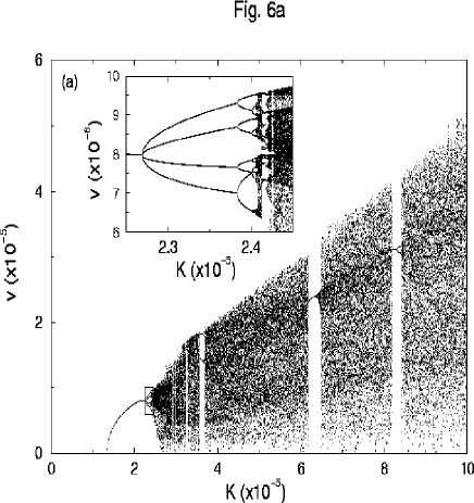
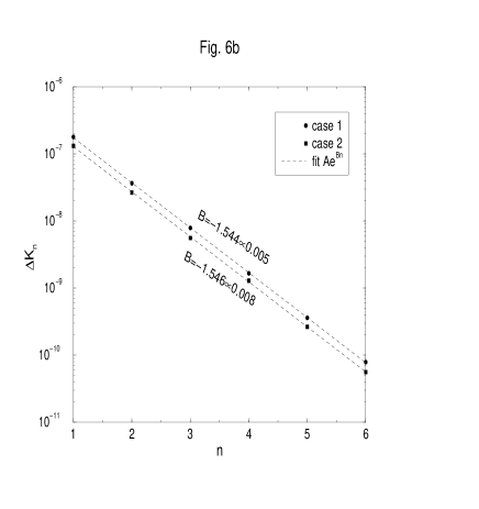
FIG. 6.: The bifurcation behavior of the radiative map (in the strong magnetic field limit). (a) The velocity $v$ versus the kicking strength $K$. The inset shows an enlargement of the indicated rectangle. (b) The spacing between the consecutive bifurcation points, $\Delta K_{n}$, versus the bifurcation number, of two different cases (as mentioned in the text). The dashed line is the exponential fit of the two cases.

The series of bifurcation points is connected to the universal constant $\delta\approx 4.6692$, which was discovered by Feigenbaum [16]. The bifurcation phenomenon is one of the signs of chaotic behavior. In Fig. 6b we present the exponential decaying behavior of the displacement between bifurcation points, $\Delta K_{n}$, in the inset of Fig. 6a (case 1) as well as, for another bifurcation region ($K=8.25\times 10^{-5}-8.45\times 10^{-5}$ denoted as case 2). As can be seen, in the two cases the exponent is almost the same, $B\approx-1.545$. The connection between the exponent $B$ and universal constant $\delta$ is given by,

$${{\Delta K_{n}}\over{\Delta K_{n+1}}}=e^{-B}=e^{1.545}\approx 4.688\approx\delta=4.6692$$ (87)

According to Feigenbaum [16] the convergence to the universal constant $\delta$ should be when $n\to\infty$ (in $\Delta K_{n}$). However, in the present case the convergence is rapid; the fitting of the exponential function is from the second bifurcation point.

The evolution of the chaotic behavior as a function of the kicking strength, $K$, is shown in Fig. 7 (the initial conditions are $V_{x,0}=0$, $V_{y,0}=10^{-5}$ and the parameters values are $B=5\times 10^{11}{\rm T}$, $q=4$; each figure contains 10000 points). In Fig. 7a there are two separate regions which become closer for increasing $K$, and finally join to one region (Fig. 7d). Moreover, the attractor occupies more area of the velocity space. The complexity of the attractor seems to be richer for larger $K$ values. However, the fractal dimension of the attractors of Fig. 7 do not increase monotonically [17]. The fractal dimension of Fig. 7 is summarized in Table I. We have calculated the fractal dimension, $D_{2}$, using two different methods, the generalized information dimension (column 2 in Table I) and the generalized correlation dimension (column 3 in Table I). The fact that the value of the fractal dimension is not an integer number is another indication for the chaotic behavior of the system. The higher the fractal dimension is, the greater is the complex behavior. Additionally, the non-integer fractal dimension indicates at least one positive Lyapunov exponent, (using the above arguments, there are three positive Lyapunov exponents) which is another indicator of chaotic behavior.

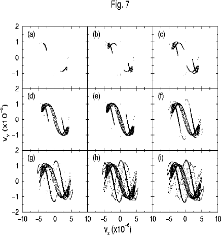
FIG. 7.: The chaotic attractors of increasing $K$ values: (a) $K=2.45\times 10^{-5}$, (b) $K=2.5\times 10^{-5}$, (c) $K=2.55\times 10^{-5}$, (d) $K=2.6\times 10^{-5}$, (e) $K=2.65\times 10^{-5}$, (f) $K=2.7\times 10^{-5}$, (g) $K=2.75\times 10^{-5}$, (h) $K=2.8\times 10^{-5}$, and (i) $K=2.85\times 10^{-5}$. For larger $K$ values the attractor occupied larger area of the velocity space.

One of the signs of chaotic behavior is the folding-stretching phenomenon, as well as the self-similarity of the map [19]. Fig. 8 shows the “inner view” of Fig. 7b. Each figure is an enlargement of the previous indicated rectangle, and contains 10000 points. The self-similar structure is clearly seen from Fig. 8c and 8d. The location of the “attractor lines” seems to form a Cantor set which is usually observed in chaotic maps. The folding-stretching phenomenon which is connected to the self-similar structure can be seen, for example, in Fig. 8d where the solid rectangle shows sharp turns of the maps. The Cantor set nature of the attractor lines is demonstrated in Fig. 9 where we choose a horizontal cut of Fig. 8a. There are more dense regions and empty regions, as expected. The inset of the figure shows that this behavior continues at smaller scales.

Fig. #	Info. D.	Corr. D.
a	1.20	1.13
b	1.32	1.27
c	1.41	1.39
d	1.43	1.43
e	1.39	1.41
f	1.36	1.36
g	1.38	1.32
h	1.47	1.49
i	1.52	1.53

TABLE I.: The fractal dimension, $D_{2}$, of Fig. 7. The first column is the figure number, the second column is the information dimension, and the third column is the correlation dimension.

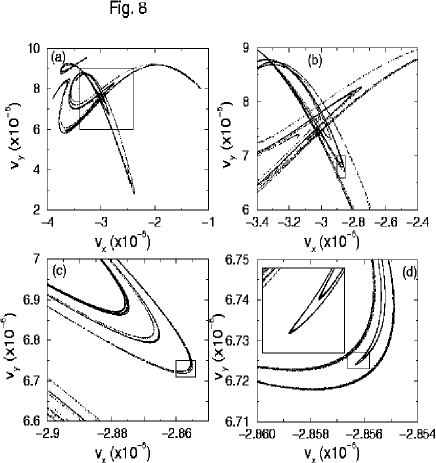
FIG. 8.: The self-similarity and the folding-stretching phenomenon (starting from Fig. 7b). Each figure is an enlargement of the indicated rectangle of the previous figure.

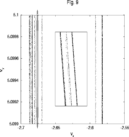
FIG. 9.: The Cantor set like behavior of the chaotic map. The inset shows the self-similarity of the attractor, keeping the Cantor set behavior of the lines.

For large kicking strength the particle increases (or decreases) its velocity to a region which balances between the kicking and the radiation. In Fig. 10 an example for the limited map is shown (the parameters values are: $B=5\times 10^{11}$, $q=4$, $K=30$, $v_{x,0}=0$, and $v_{y,0}=0.99$). The clear boundaries are caused by the radiation which decreases the velocity significantly before the next kick. The kicking pushes the particle toward light velocity; the gap between light velocity and the attractor boundaries is approximately the energy loss caused by the radiation. The self-similar behavior and the strength-folding phenomenon can be seen in the inset of Fig. 10.

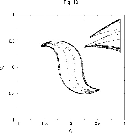
FIG. 10.: The chaotic behavior of the radiative map (large $B$) for large kicking strength.

VIII Intermediate magnetic field

In the previous sections the analysis of the weak and the strong magnetic field was discussed. In this section we will discuss the intermediate magnetic field strength regime. Basically, a numerical integration of Eq. (35) should be performed. However, the approximation for the weak magnetic field (Eqs. (63)-(66) is valid up to $B=10^{10}{\rm T}$ , and thus one can avoid the numerical integration.

In Fig. 11 some of the possibilities that can appear in the intermediate magnetic field regime are presented. For example, Fig. 11a shows a destroyed web like structure, i.e., the particle started to diffuse through a web structure, but after a sufficiently large number of iterations it either decays toward zero velocity, or stops its acceleration and iterates in a quasiperiodic motion (see the enlargement of the indicated rectangle in Fig. 11a, where the particle decays towards a periodic orbit). The particle starts near an unstable fixed point (Eq. (71)), and since the magnetic field is relatively high its influence on the particle is larger and it decays inside. For smaller magnetic field the particle diffuses through the filaments of the web. In might be that, if the initial condition were chosen closer to the unstable fixed point, the particle would diffuse. A supported example for that claim can be seen in Fig. 11b where the particle starts from smaller velocity (half of the velocity of Fig. 11a) using the same parameters values as in Fig. 11a (and thus the approximation of Eq. (71) is more accurate) and it diffuses to the high velocity regime (approximately, to a ten times larger velocity). Thus, one can safely conclude that for intermediate magnetic field the influence of the unstable fixed point is somehow weaker, and it is more difficult to observe the web structure. Or, to state it in a different way, the width of the filament is narrower when the magnetic filed is stronger.

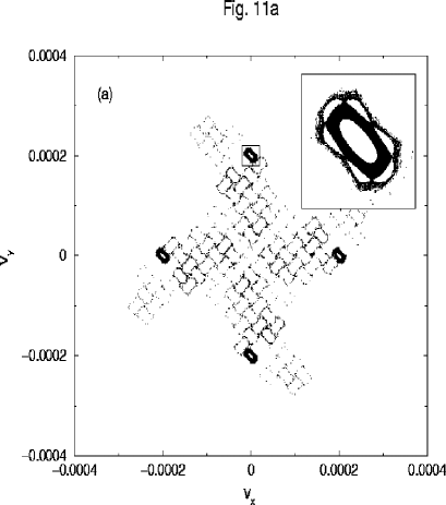
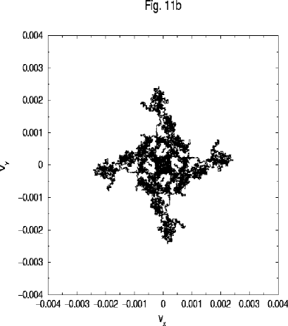
FIG. 11.: The intermediate magnetic field regime. The parameter values are $B=5\times 10^{6}{\rm T}$, $q=4$, $K=10^{-5}$, and $v_{x,0}=0$. Each figure consist $10^{5}$ points. The initial velocity, $v_{y,0}$, in (a) is $2\times 10^{-5}$ while in (b) is $1\times 10^{-5}$.

IX Summary

In the present paper we have investigated the effect of radiation on the stochastic web. Under the restriction of small magnetic fields ($B\lesssim{\cal O}(100T)$) an iterative map was constructed. Moreover, the effect of radiation on the stochastic web is very small because of the small magnetic field. Qualitatively, the non-radiative and the radiative cases have similar web structure. Despite of the naive expectation that the diffusion rate in the radiative case should be smaller than non-radiative case, one can find cases in which the opposite effect is observed.

Although it seems the effect of radiation is not qualitatively significant under laboratory conditions, it have a strong effect in the presence of a strong magnetic field. Such a magnetic field could occur near or in a neuron star (or other heavy stars) and it can cause a large radiation correction to the motion of the particle. An iterative map was constructed for that regime also. It was found that the web structure disappears and is replaced by rich chaotic behavior which is demonstrated by the non-integer fractal dimension, bifurcation, self-similarity, and folding and stretching. The chaotic attractor occupies a small part of the velocity space, and practically means that the particle can not accelerate to infinite energy, as in the regular stochastic web. This chaotic behavior seems to be a “robust” chaotic behavior (implying that one can find chaotic behavior using slightly different parameter values).

For the intermediate magnetic field strength, the influence of the unstable fixed point is smaller relative to a weaker magnetic field.

X Acknowledgements

We would like to thank I. Dana and A. Priel at Bar Ilan University, for helpful discussions, and S. Cohen and R. White for their interesting comments at a seminar at the Princeton Plasma Physics Laboratory where some of these results were presented. One of us (LPH) wishes to thanks S.L. Adler for his kind hospitality at the Institute for Advanced Study, where this work was completed.

REFERENCES

- [1] email-address: ashkenaz@mail.biu.ac.il
- [2] On leave from School of Physics and Astronomy, Raymond and Beverly Sackler Faculty of Exact Sciences, Tel Aviv University, Ramat Aviv, Israel, and Department of Physics, Bar Ilan University, Ramat Gan, Israel. email-address: larry@post.tau.ac.il
- [3] G.M. Zaslavskii, M.Yu. Zakharov, R.Z. Sagdeev, D.A. Usikov, and A.A. Chernikov, Zh. Eksp. Teor. Fiz 91, 500 (1986) [Sov. Phys. JEPT 64, 294 (1986)].
- [4] V.I. Arnold’d, Dokl. Akad. Nauk. SSSR 159, 9 (1964).
- [5] A.A. Chernikov, T. Tel, G. Vattay, and G.M. Zaslavskii, Phys. Rev. A 40, 4072 (1989).
- [6] D.W. Longcope and R.N. Sudan, Phys. Rev. Lett. 59, 1500 (1987); See also, A.J. Lichtenberg and M.A. Lieberman, Regular and Chaotic Dynamics 2nd ed., (Springer-Verlag, New York, 1992).
- [7] H. Karimabadi and V. Angelopoulos, Phys. Rev. Lett. 62, 2342 (1989).
- [8] We thank T. Goldman for comments on the mechanism for this bound in our equation during a seminar at Los Alamos.
- [9] L.P. Horwitz and Y. Ashkenazy, To be published in Discrete Dynamics in Nature and Society.
- [10] M. Abraham, Theorie der Elektrizität, vol. II, (Springer, Leipzig, 1905). See ref. [12] for a discussion of the origin of these terms; P.A.M. Dirac, Proc. Roy. Soc. London Ser. A, 167, 148 (1938).
- [11] A.A. Sokolov and I.M. Ternov, Radiation from Relativistic Electrons (Amer. Inst. of Phys. Translation Series, New York, 1986).
- [12] F. Rohrlich, Classical Charged Particles (Addison Wesley, Reading, Mass., 1965).
- [13] J.M. Aguirrebiria, J. Phys. A Math. Gen. 30, 2391 (1997).
- [14] E. Barreto, B.R. Hunt, C. Grebogi, and G.M. Yorke, Phys. Rev. Lett. 78, 4561 (1997).
- [15] S. Banerjee, J.A. Yorke, and C. Grebogi, Phys. Rev. Lett. 80, 3049 (1998).
- [16] M.J. Feigenbaum, J. Stat. Phys. 19, 25 (1978).
- [17] For details about the calculation of the generalized information dimension and the generalized correlation dimension see Y. Ashkenazy, “The Use of Generalized Information Dimension in Measuring Fractal Dimension of Time Series”, To be published in Physica A, chao-dyn/9805001.
- [18] J.L. Kaplan and J.A. Yorke, Comm. Math. Phys. 67, 93 (1979).
- [19] J. Guckenheimer and P. Holmes, Nonlinear Oscillations, Dynamical Systems, and Bifurcations of Vector Fields (Springer-Verlag, New York, Berlin, Heidelberg, Tokyo, 1983).