Quasilinear theory of collisionless Fermi acceleration in a multicusp magnetic confinement geometry

Abstract

Particle motion in a cylindrical multiple-cusp magnetic field configuration is shown to be highly (though not completely) chaotic, as expected by analogy with the Sinai billiard. This provides a collisionless, linear mechanism for phase randomization during monochromatic wave heating. A general quasilinear theory of collisionless energy diffusion is developed for particles with a Hamiltonian of the form $H_{0}+H_{1}$, motion in the unperturbed Hamiltonian $H_{0}$ being assumed chaotic, while the perturbation $H_{1}$ can be coherent (i.e. not stochastic). For the multicusp geometry, two heating mechanisms are identified — cyclotron resonance heating of particles temporarily mirror-trapped in the cusps, and nonresonant heating of nonadiabatically reflected particles (the majority). An analytically solvable model leads to an expression for a transit-time correction factor, exponentially decreasing with increasing frequency. The theory is illustrated using the geometry of a typical laboratory experiment.

52.50.Gj,05.45.+b,52.20.Dq,52.55.Lf

I Introduction

The quasilinear diffusion equation in its original form (QLT1) was a Fokker-Planck equation describing the velocity-space diffusion of particles due to random scattering by waves. In the absence of the waves the plasma was assumed to be infinite and homogeneous so that the unperturbed motion was rectilinear. The diffusion equation was derived [1, 2, 3] from the Vlasov equation by solving for the perturbed part of the distribution function, in the linear approximation and assuming the unperturbed distribution function to be essentially constant over the timescale of wave-particle interaction, then substituting back into the full Vlasov equation and averaging over position (or, equivalently, over the random phases of the waves).

To put this formalism in a more general perspective, it is advantageous to cast it in Hamiltonian form, with the particle motion in the absence of waves being described by an unperturbed Hamiltonian $H_{0}$. The total single-particle Hamiltonian is then $H_{0}+\epsilon H_{1}$, with the waves being incorporated in the perturbation Hamiltonian $H_{1}$. In QLT1, all stochasticity comes from the assumption of random phases in the assumed broad spectrum of waves in $H_{1}$. The smallness parameter $\epsilon$ expresses the assumption that the amplitudes of individual waves are small, so that the short-time-scale perturbations to the distribution function can be derived using linear, $O(\epsilon),$ theory (hence the terminology “quasilinear”). The only nonlinear effect is the long-time diffusion described by the diffusion coefficient, which is $O(\epsilon^{2})$ .

It is not really necessary to assume an infinite, homogeneous plasma. The essence of QLT1 is the assumption that $H_{0}$ is integrable, so that a canonical transformation to action-angle coordinates exists. Then the unperturbed motion in angle space is rectilinear, just as that in coordinate space in the case of a homogeneous medium. This action-angle generalization was carried out by Kaufman [4] and by Hazeltine et al. [5] to derive a quasilinear diffusion equation (in action space) for wave-particle scattering in axisymmetric toroidal magnetic confinement geometries (e.g. tokamaks). The formalism has been used, for example [6], to investigate the effect of a sheared radial electric field on anomalous transport in a tokamak.

With the development of the theory of Hamiltonian chaos it has come to be realized that a quasilinear diffusion equation can also be derived in cases where $H_{1}$ represents the effect of a coherent wave, provided the interaction of $H_{0}$ and $H_{1}$ produces a chaotic motion. We call this form of quasilinear theory QLT2, and it is very useful in the theory of radio-frequency (rf) and microwave heating of plasmas [7] because this is typically done with coherent waves.

Again, $H_{0}$ is assumed integrable so that an action-angle transformation exists. In these theories the perturbation is still the source of chaos (“intrinsic stochasticity”), which causes the action variables, constructed in the integration of $H_{0}$, to perform the random walk described by the quasilinear diffusion equation. Assuming the Hessian matrix $\partial^{2}H_{0}/\partial p_{i}\partial p_{j}$ to be nonsingular, the coherent perturbation must exceed a certain amplitude for global resonance overlap, and hence chaos, to occur [8, 9, 10]. Thus, paradoxically, a criterion for QLT2 to apply is that the system be sufficiently nonlinear!

In the present paper we examine a third form of quasilinear theory, which we call QLT3. This case is the complete obverse of the original quasilinear diffusion problem: we now assume the unperturbed Hamiltonian $H_{0}$ to be completely nonintegrable, giving rise to strongly chaotic motion in the unperturbed system. The chaotic dynamics of the unperturbed Hamiltonian system then provides randomization and allows the application of a quasilinear formalism to derive the diffusion equation for the distribution function.

Of course, since $H_{0}$ is not integrable, an action-angle representation does not exist. In fact we assume $H_{0}$ to be so strongly chaotic that the unperturbed motion covers essentially the entire energy surface $H_{0}={\mathcal{E}}$ ergodically, except as restricted by integrals of the motion associated with any continuous symmetries of $H_{0}$. The goal of this paper is to determine the diffusion in ${\mathcal{E}}$ caused by the time-dependent perturbation $H_{1}$.

Since the unperturbed motion provides the source of stochasticity (with no threshold), we can, as in QLT2, assume the perturbation to be coherent. Thus the theory is applicable to wave heating of plasmas in strongly nonintegrable magnetic confinement geometries.

The assumption of uncorrelated gyrophase in successive passes through the resonance region is often made in the derivation of a quasilinear diffusion equation to describe cyclotron resonance heating of magnetically confined plasmas. However, in simple confinement geometries, such as magnetic mirrors, $H_{0}$ is essentially integrable owing to the existence of the adiabatic invariant $\mu$ and another integral due to symmetry, or a second adiabatic invariant. Lichtenberg and Lieberman [11] have analyzed collisionless heating in such systems using area-preserving maps, and find the random phase assumption to be valid only well beyond the nonlinear threshold where the last invariant circle is destroyed and chaotic motion becomes global. In our nomenclature, quasilinear diffusion in these systems is an example of QLT2, not QLT3.

On the other hand, in systems with a null in the magnetic field $\mu$ is not globally conserved and the situation is rather different from that in the much-studied mirror systems. For instance, Yoshida et al. [12] have recently studied rf heating in a two-dimensional slab model with a neutral line, where $\mu$ conservation is broken. They find heating due to the onset of chaos at finite amplitude of the perturbing field. However, their unperturbed system has two symmetry directions, and thus their $H_{0}$ is integrable, despite the breaking of the adiabatic invariant. Thus their model must be classified as a QLT2 case also.

In systems with a null in the magnetic field and only one symmetry direction, however, $H_{0}$ is not in general integrable. An important class of such systems are the magnetic cusp confinement geometries, which are much used in low-temperature plasma physics due to the ease with which they can be created with arrays of permanent magnets [13][14, pp. 146–150]. In this paper we give evidence that they fulfill the criterion for systems of type QLT3 in that their unperturbed dynamics is almost completely chaotic.

We know from the work of Sinai [15, 16] that particle motion on a billiard table with a convex boundary is a strongly chaotic system due to the defocussing effect of each collision with this boundary. In fact Sinai showed the motion to be strongly mixing, so that ergodic theory could be applied. This suggests that cusp confinement systems, where magnetic fields lie on surfaces that are convex toward the plasma, are strongly chaotic. Indeed the four-cusp Hamiltonian $H=\mbox{$\frac{1}{2}$}(p_{x}^{2}+p_{y}^{2}+x^{2}y^{2})$ was at one time conjectured to be completely chaotic like a Sinai billiard. Although Dahlqvist and Russberg [17] disproved this conjecture by finding a stable periodic orbit, they found that the island of stability surrounding this orbit was extremely small, so for practical purposes one can assume that the energetically accessible phase space is covered ergodically in this system.

In this paper we study a magnetic field configuration consisting of a “picket fence” of infinite linear magnetic dipoles, producing multiple line cusps. This can be regarded as a simplified model for a low-temperature plasma source, created using arrays of permanent magnets [18, 19]. It is also a rather simple model, in which the unperturbed dynamics can be simplified analytically to a considerable extent by the use of complex variable theory.

In the limit of a large number of dipoles the interior of the plasma is essentially free of magnetic field and the unperturbed motion is rectilinear in the interior region, while near the edge of the confinement region, a particle can be reflected over a range of angles. Thus we might expect the configuration to approximate a chaotic billiard problem. (In the original Sinai problem the convex boundary was in the interior of the domain, whereas the billiard analog of the present example has an outer boundary that is convex except for cusps, like the “bow-tie” billiard shown in Fig. 7.24(e) of Ref. [16].)

The problem is also related to a model originally proposed by Fermi [20, 21, 22] for explaining the acceleration of cosmic rays to the extraordinarily high energies observed. In the Fermi model the cosmic ray particles move rectilinearly except during occasional collisions with moving magnetized clouds of gas, which cause diffusion in energy space. The present model includes both the possibility of cyclotron-resonance heating in the mirror-like cusp regions and nonresonant heating of particles reflected without penetrating deeply into the cusps. The latter case is much closer to the original Fermi problem and is the main focus of the paper.

In Sec. II we introduce the confinement geometry and unperturbed Hamiltonian in detail, and in Sec. III we analyze the dynamics of this system and show it is indeed strongly chaotic for the class of particles (“free particles”) that traverse the central low-field region. However, in Sec. III D 3 we produce a counter example to any conjecture that the motion is totally chaotic by finding a stable periodic orbit.

In Sec. IV we introduce the wave-particle interaction. The general quasilinear diffusion equation is derived in Sec. V. An analytically solvable one-dimensional model of the magnetic field is used in Sec. VI to estimate heating of nonadiabatically reflected particles. The result is of the form expected from simple Fermi acceleration theory multiplied by a transit-time reduction factor that becomes exponentially small when the transit time is much longer than the period of the applied field. The theory is discussed using typical parameters for permanent-magnet confinement experiments in Sec. VII.

II Unperturbed Hamiltonian

A Two-dimensional magnetic Hamiltonian

The behavior of a sufficiently dilute plasma can be analyzed on the basis of single-particle motion in magnetic and electric fields made up of an externally imposed component and an internally generated component produced by the collective currents and charges from the combined effect of many otherwise noninteracting particles. In this paper we suppose that the self-consistent component is negligible and analyze single-particle motion in an imposed magnetic field.

Consider the motion of a particle of charge $q$ and mass $m$ in a straight, infinitely long magnetic confinement system with vector potential ${\mathbf{A}}=\psi(x,y){\mathbf{e}}_{z}$, where $x$, $y$ and $z$ are Cartesian coordinates and ${\mathbf{e}}_{z}$ is the unit vector in the $z$-direction. The magnetic field is $B_{x}=\partial\psi/\partial y$, $B_{y}=-\partial\psi/\partial x$, $B_{z}=0$, so contours of the flux function $\psi(x,y)$ in any plane $z={\mathrm{const}}$ define magnetic field lines.

The Hamiltonian is (see e.g. [23])

$$H_{0}=\frac{p_{x}^{2}}{2m}+\frac{p_{y}^{2}}{2m}+\frac{[p_{z}-q\psi(x,y)]^{2}}{2m}\;,$$ (1)

where $p_{i}$ ($i\in\{x,y,z\}$) are the canonical momenta, Hamilton’s equations of motion being $\dot{x}_{i}=\partial H_{0}/\partial p_{i}$, $\dot{p}_{i}=-\partial H_{0}/\partial x_{i}$.

B Multicusp flux function

Assuming no currents present in the plasma, $\psi$ obeys Laplace’s equation. It is a standard result that two-dimensional solutions of Laplace’s equation can be constructed by taking the real or imaginary part of any analytic function of $\zeta\equiv x+iy$ [24]. Thus we write

$$\psi(x,y)={\mathrm{Re}}\,\Psi(\zeta)\;,$$ (2)

where $\Psi(x,y)$ is the complex flux function.

For instance, a line current (line magnetic monopole) at $\zeta_{0}$ is represented by the real (imaginary) part of $\ln(\zeta-\zeta_{0})$.

Although a magnetic monopole cannot be realized in nature, a magnet can be modeled as a superposition of magnetic dipoles. We consider a magnet that is long in the $z$-direction, thin in the $x$- and $y$-directions, and magnetized in the $x$-direction so that it can be modeled by a line magnetic dipole. Such a linear dipole can be produced by differentiation of ${\mathrm{Im}}\,\ln(\zeta-\zeta_{0})$ with respect to $x_{0}$.

Superimposing the flux functions for $2n$ linear magnets of strength alternately $+K$ and $-K$ lying in a circular cylinder of radius $a$ about the $z$-axis we find $\psi$ for a circular multidipole magnetic confinement system,

$$\psi = K\,{\mathrm{Im}}\,\sum_{n^{\prime}=0}^{n-1}\left[\frac{u_{n}^{4n^{\prime}+1}}{\zeta-au_{n}^{4n^{\prime}+1}}-\frac{u_{n}^{4n^{\prime}-1}}{\zeta-au_{n}^{4n^{\prime}-1}}\right]\;,$$ (3)

$$= \frac{2nK}{a}{\mathrm{Re}}\,\,\left[\left(\frac{\zeta}{a}\right)^{n}+\left(\frac{a}{\zeta}\right)^{n}\right]^{-1}\;.$$ (4)

Here $u_{n}\equiv\exp(\pi i/2n)$ is the $4n$th root of unity. The equivalence of the first and second forms can be verified by showing that they have the same poles and residues and the same value at $\zeta=0$.

Thus, comparing with Eq. (2), we see that the complex stream function for a circular dipole picket fence is given by

$$\Psi = \frac{2nK}{a}\left[\left(\frac{\zeta}{a}\right)^{n}+\left(\frac{a}{\zeta}\right)^{n}\right]^{-1}$$ (5)

$$\equiv \frac{nK}{a}\,{\mathrm{sech}}\,\!\left[n\ln\left(\frac{\zeta}{a}\right)\right]\;.$$ (6)

It is clear from the first form that $\Psi$ has poles at the $2n$th roots of $-a^{2n}$. In terms of polar coordinates $r$ and $\theta$ such that $\zeta=r\exp i\theta$, the poles are at $r=a$, $\theta=\pi/2n+2l\pi$, $l=0,\,1,\ldots,2n-1$. Contours of $\psi$ (lines of force) are shown in Fig. 1 for the case $n=6$, with distances measured in units of $a/n$.

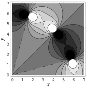
FIG. 1.: Contours of the flux function for a typical cylindrical multicusp geometry produced by 12 line dipoles of alternating polarity.

C Near field and nondimensionalization

We now consider the behavior of $\psi$ in the region between two magnets, which for definiteness we take to be those immediately above and below the positive real $x$-axis. We expand about the point $\zeta=a$, on the circle on which the magnets are located, by setting $\zeta=a+\xi$, where $\xi\equiv x-a+iy$. Assuming $|\xi|\ll a$, we see from Eq. (6) that

$$\Psi\approx\frac{nK}{a}\,{\mathrm{sech}}\,\!\left(\frac{n\xi}{a}\right)\;.$$ (7)

Thus, on the $x$-axis $\psi$ peaks at $x=a$ and it decays rapidly on either side. Furthermore, we see that the scale length of the $x$ and $y$ variation is not $a$ but $a/n$. In Sec. III D 1 we shall encounter Eq. (7) again in the context of the asymptotic limit $n\rightarrow\infty$.

Expanding $\Psi$ to second order in $n\xi/a$ we find $\psi\equiv{\mathrm{Re}}\,\Psi\approx\psi_{\mathrm{X}}\{1-n^{2}[(x-a)^{2}-y^{2}]/2a^{2}\}$ in the neighborhood of $(a,0)$, where

$$\psi_{\mathrm{X}}\equiv nK/a$$ (8)

is the value of $\psi$ at this saddle point, the location of a magnetic-field null. It is also useful to define a typical magnetic field $B_{0}$ in the strong-field region via the relation $B_{0}\equiv n\psi_{\mathrm{X}}/a$.

We term the energy of a particle with momentum ${\mathbf{p}}=0$ located at this saddle point the escape energy

$${\mathcal{E}}_{\mathrm{esc}}\equiv\frac{q^{2}\psi_{\mathrm{X}}^{2}}{2m}\equiv\frac{1}{2m}\left(\frac{qnK}{a}\right)^{2}\;.$$ (9)

In all numerical work and figures in this paper we nondimensionalize by measuring distance in units of $a/n$, mass in units of $m$, time in units of the typical inverse angular cyclotron frequency

$$\tau_{\mathrm{X}}\equiv\frac{m}{|q|B_{0}}\equiv\frac{a^{2}m}{n^{2}Kq}\;,$$ (10)

and charge in units of $|q|$. In these units $a=n$, $m=|q|=\tau_{\mathrm{X}}=\psi_{\mathrm{X}}=B_{0}=1$, and ${\mathcal{E}}_{\mathrm{esc}}=\mbox{$\frac{1}{2}$}$.

III Unperturbed particle dynamics

A Dynamics in complex notation

For a given $p_{z}$, the dynamics is a two-degree-of-freedom autonomous Hamiltonian system which can be compactly written using complex notation as

$$\dot{\zeta} = \frac{1}{m}\,p_{\zeta}\;,$$ (11)

$$\dot{p}_{\zeta} = \frac{q}{m}\left[p_{z}-q{\mathrm{Re}}\,\Psi(\zeta)\right][\Psi^{\prime}(\zeta)]^{*}\;,$$ (12)

where the prime on $\Psi$ means the derivative with respect to its argument, $*$ means complex conjugate, and $p_{\zeta}\equiv p_{x}+ip_{y}$.

B Integrability and effective potential

Because $H_{0}$ is independent of $z$, $p_{z}$ is a constant of the motion. Also, $H_{0}$ itself is a constant of the motion, $H_{0}={\mathcal{E}}$, where the constant ${\mathcal{E}}$ is the total energy. However, the absence of a third integral of the motion means the system is not integrable. Thus we must resort to numerical integration to investigate the nature of the unperturbed orbits.

Before proceeding to a discussion of the numerical results, however, we observe that some qualitative understanding of the motion can be found by determining the bounds of the motion implied by the constancy of $H_{0}$. Inspecting Eq. (1) we see that the term $V_{\mathrm{eff}}\equiv(p_{z}-q\psi)^{2}/2m$ in $H_{0}$ acts as an effective potential in which the particles move. The motion in the $(x,y)$-plane is thus bounded by the curves $V_{\mathrm{eff}}(x,y)={\mathcal{E}}$. Note that $V_{\mathrm{eff}}\geq 0$, with equality occurring on the contours $\psi=p_{z}/q$. Also, since $\psi$ vanishes at the origin, $V_{\mathrm{eff}}=p_{z}^{2}/2m$ there.

In the case $p_{z}=0$, the curves $V_{\mathrm{eff}}(x,y)={\mathrm{const}}$ are just level curves of $|\psi|$. There are thus two cases:

1. Perfect confinement
   ${\mathcal{E}}<{\mathcal{E}}_{\mathrm{esc}}$, the curve $|\psi|=(2m{\mathcal{E}})^{1/2}/|q|$ encloses the origin (though it has cusps at the magnets) and there is thus no leakage of particles with $p_{z}=0$ through the dipole picket fence.

2. Partial confinement
   For ${\mathcal{E}}>{\mathcal{E}}_{\mathrm{esc}}$, the curves $|\psi|=(2m{\mathcal{E}})^{1/2}/|q|$ are disjoint and thus particles can escape through the “mountain passes” (see Fig. 1) between the magnets.

In either case the particles are free to traverse a large region including the origin, like particles rolling on a billiard table [in case (ii) it is a billiard table with pockets]. We refer to particles on such orbits as free particles, to be contrasted with the trapped particles discussed in the next section.

FIG. 2.: A typical trapped-particle orbit in the magnetic field shown in Fig. 1. The thick lines show the boundaries of the energetically accessible regions.

C Trapped-particles

For $p_{z}\neq 0$ a new class of orbit arises, the trapped particles. This occurs when the energy is less than the value of $V_{\mathrm{eff}}$ at the origin, i.e. when ${\mathcal{E}}<p_{z}^{2}/2m$, for then the low-magnetic-field central region is energetically inaccessible (see Sec. III D) and the particle must be confined in the edge region near the magnets, as illustrated in Fig. 2.

Because deeply trapped particles are always in a region of strong magnetic field, their dynamics can be analyzed (see, e.g., [23, pp. 21–22]) by decomposing the motion into that of the guiding center, with velocity ${\mathbf{v}}=v_{\parallel}{\mathbf{B}}/B+\mathrm{drifts}$, and a gyro motion with velocity ${\mathbf{v}}_{\perp}$ in the plane locally orthogonal to ${\mathbf{B}}$. The adiabatic invariant

$$\mu\equiv\frac{mv_{\perp}^{2}}{2B}\;,$$ (13)

is conserved to high degree of approximation, providing an approximate third integral of the motion. The unperturbed dynamics of this class of orbit is thus quasi-integrable, not chaotic, implying that we must use quasilinear theory of type QLT2 to derive a diffusion equation (i.e. heating will occur only beyond a nonlinear amplitude threshold). Cyclotron resonance heating in mirror geometries has been much discussed in the literature [14, pp. 413–422] and we shall not discuss the heating of the trapped particles in this paper.

D Free particles

For a given energy ${\mathcal{E}}$ and conserved momentum $p_{z}$, the energetically accessible region is the set of points $(x,y)$ for which there exist $p_{x}$ and $p_{y}$ such that $H_{0}(x,y,p_{x},p_{y},p_{z})={\mathcal{E}}$. From Eq. (1) we get the inequality

$$[p_{z}-q\psi(x,y)]^{2}\leq 2m{\mathcal{E}}\;.$$ (14)

We define the free particles as those for which the origin is energetically accessible. Thus, since $\psi(0,0)=0$, Eq. (14) implies that free particles are those for which

$$p_{z}^{2}\leq 2m{\mathcal{E}}\;.$$ (15)

The total region accessible to free particles is the set of $(x,y)$ for which the ranges of $p_{z}$ defined by Eq. (14) and Eq. (15) are not disjoint. This gives the condition

$$|q\psi(x,y)|\leq 2(2m{\mathcal{E}})^{1/2}\;.$$ (16)

This inequality being satisfied, the intersection of the ranges defined by Eq. (14) and Eq. (15) is $[q\psi-(2m{\mathcal{E}})^{1/2},(2m{\mathcal{E}})^{1/2}]$ for $q\psi>0$, or $[-(2m{\mathcal{E}})^{1/2},q\psi+(2m{\mathcal{E}})^{1/2}]$ for $q\psi<0$.

A typical trajectory for a free particle with energy well below the escape energy is shown in Fig. 3. In this case $p_{z}=0$, and the initial conditions are $x_{0}=y_{0}=0$, $p_{x0}=0.04$, $p_{y0}=0.05$, giving ${\mathcal{E}}=0.00205$.

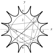
FIG. 3.: A typical free-particle orbit in the magnetic field shown in Fig. 1, with initial conditions as described in the text.

We see that the energetically accessible region is bounded by a series of curves (shown as thick lines) joining in cusps at the magnets. These bounding curves are convex toward the confinement region, except at the cusps, where the magnetic field goes to infinity so that no particle can penetrate. Also we see that the motion of the particle well away from the bounding curves is approximately rectilinear so that the system does indeed appear like a physical realization of a Sinai billiard system [15].

Although the orbit in Fig. 3 looks chaotic, a better test for chaos is to do a Poincaré surface of section puncture plot, as shown in Fig. 4 for a particle with $p_{z}=0$ and energy ${\mathcal{E}}=0.0017$ started near the periodic orbit described in Sec. III D 3. The Poincaré surface of section is $x>0$, $y=0$ and its images under the symmetry operation $\zeta\mapsto\exp(i\pi/6)\zeta$. Dots indicate both upward- and downward-going passes of the orbit. It is seen that the orbit appears to fill the energetically accessible phase space ergodically, indicating strong chaos.

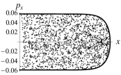
FIG. 4.: Intersections of an orbit with the Poincaré surface of section $y=0$ described in the text.

However, the interaction with the field near the bounding curve is not specular reflection with a zero radius of curvature, so our magnetic cusp confinement system is not precisely analogous to that studied by Sinai. In fact, studying Fig. 3 we see that there are two qualitatively different kinds of reflection event — approximately specular reflection with a small-but-finite radius of curvature, and “sticky reflections” near the cusps, where the particle is temporarily trapped in a one-sided mirror field and oscillates several times before reflection. As explained below, we call these nonadiabatic and adiabatic reflections, respectively.

1 Scattering analysis of reflection, large $n$

In order to make the reflection process a precisely defined event we go to the large-$n$ limit, in which the spacing between the magnets, $\pi a/n$, and the scale length of magnetic field variation, $a/n$, become small compared with the radius $a$. Since we are interested in dynamics near the wall of magnets, we shift the origin to the saddle point at $\zeta=a$ by defining $\xi\equiv\zeta-a$, just as in Sec. II C. Again Eq. (7) applies at leading order, but this time its region of validity extends beyond the region of the magnetic null to include the high-field regions near the magnets (the only requirement being $|\xi|\ll a$).

We now take Eq. (7) to be the exact complex flux function for the model problem of an infinite line of magnets (treating $n$ as an arbitrary parameter, which is scaled out in the nondimensionalization defined in Sec. III B). A reflection event is now precisely defined as a scattering process, in which a particle impinges from ${\mathrm{Re}}\,\xi=-\infty$ (where the orbit is asymptotically a straight line), reflects off the magnetic field of the magnets, then retreats back toward ${\mathrm{Re}}\,\xi=-\infty$.

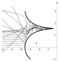
FIG. 5.: A set of nine orbits, incident in the direction normal to the line of magnets, with different “impact parameter” $y_{0}$. The thick line shows the boundary of the energetically accessible region. The origin of the $x$-axis has been shifted to lie on the line of magnets.

In Fig. 5 we illustrate some typical reflection events for particles with initial momentum $p_{0x}=0.06$, $p_{y0}=0$, $p_{z}=0$, giving energy ${\mathcal{E}}=0.0018$. For small initial values of $y$, $y_{0}$, the reflection is approximately specular, but as $y_{0}$ approaches $\pi/2$ (the height of the first magnet above the $x$-axis), the orbit undergoes more and more oscillations (gyrations) before being reflected back.

Clearly, for $y_{0}\approx\pi/2$ we can use adiabatic invariant theory (cf. Sec. III C) to treat the process of reflection in the mirror field in the throat of the cusp field, whereas for $y_{0}\approx 0$ the particle does not complete even one gyration about the magnetic field, so the adiabatic invariant is not defined on any part of the orbit. In order to determine on which part of any given orbit $\mu$ is approximately conserved, we compute the cyclotron frequency $f_{\mathrm{c}}\equiv\omega_{\mathrm{c}}/2\pi$ at each point on the orbit, where $\omega_{\mathrm{c}}(t)\equiv|q|B(t)/m$, and compare it with the time-rate-of-change of $\ln B$.

Suppose that the inequality $f_{\mathrm{c}}>\dot{B}/B$ holds over the interval $t_{1}<t<t_{2}$ and is violated outside the interval. Adiabatic invariance theory applies during this interval, provided the particle has enough time to execute at least one gyroorbit. To determine the latter point, we calculate the total gyrophase change over the interval in which adiabatic invariance potentially applies,

$$\Delta\phi\equiv\int_{t_{1}}^{t_{2}}\omega_{\mathrm{c}}\,dt\;.$$ (17)

Then we define an adiabatic reflection as one for which $\Delta\phi/2\pi>1$ and a nonadiabatic reflection as one for which $\Delta\phi/2\pi\leq 1$.

FIG. 6.: Adiabaticity parameter $\Delta\phi/2\pi$ vs. impact parameter times $2/\pi$ for normally incident orbits with energy $0.01$ (solid line) and very low energies (dashed line).

Figure 6 shows this adiabaticity parameter for the case of normal incidence, as depicted in Fig. 5. Two values of energy are shown, a relatively high energy ${\mathcal{E}}=0.01$ and the low-energy limit ${\mathcal{E}}\rightarrow 0$ (see below). Reflection is nonadiabatic for roughly $60\%$ of particles in both cases.

FIG. 7.: Adiabaticity parameter $\Delta\phi/2\pi$ vs. impact parameter times $2/\pi$ for orbits incident at $20^{\circ}$ to the normal with energy $0.01$ (solid line) and very low energies (dashed line).

Figure 7 shows the dependence of $\Delta\phi/2\pi$ on impact parameter $y_{0}$ for particles incident at an angle of $20^{\circ}$ to the normal in the $x$-$y$ plane, and with $p_{z}=0$. (Here $y_{0}$ is defined such that the orbits have initial values $x=X_{0}$, $y=Y_{0}+y_{0}$, where $X_{0}$ is an arbitrarily large negative constant and the constant $Y_{0}$ is chosen so that $y_{0}=0$ corresponds to an orbit symmetric about the $x$-axis.)

It is seen that the adiabatic region is much reduced in the low-energy case, and has virtually disappeared in the high-energy case. At angles of incidence greater than $25^{\circ}$, both high- and low-energy particles reflect nonadiabatically for all impact parameters. The ratio of the solid angle occupied by the cone of angles of incidence $\eta<25^{\circ}$ to the cone of all possible angles of incidence, $\eta<90^{\circ}$ is about $0.093$. Thus we conclude that considerably less than $10\%$ of particles reflect adiabatically.

The low-energy limit referred to above is defined by observing that the lower the incident energy, the larger the value of $-{\mathrm{Re}}\,\xi$ at which the particle reflects. Thus, in this limit we can replace ${\mathrm{sech}}\,(n\xi/a)$ by $2\exp(n\xi/a)$ in Eq. (7) and define the low-energy approximation as the result of replacing $\Psi$ with

$$\Psi_{\mathrm{low}}\equiv 2\psi_{\mathrm{X}}\,\exp\!\left(\frac{n\xi}{a}\right)\;,$$ (18)

where $\psi_{\mathrm{X}}$ is defined in Eq. (8).

The dynamics in this limit exhibits an important scale invariance: if we displace the orbit in the $x$-direction using the transformation $\xi=\xi^{\prime}+h$, where $h$ is a real constant, then the flux function changes by a constant factor: $\Psi_{\mathrm{low}}(\xi)=\exp(nh/a)\Psi_{\mathrm{low}}(\xi^{\prime})$. Inspecting Eq. (12) we see that the transformation ${\mathbf{p}}=\exp(nh/a){\mathbf{p}}^{\prime}$, $t=\exp(-nh/a)t^{\prime}$ leaves the form of the equations of motion invariant. The energy is transformed according to ${\mathcal{E}}=\exp(2nh/a){\mathcal{E}}^{\prime}$. Clearly $y_{0}$ is invariant and it is also easy to show from Eq. (17) that $\Delta\phi$ is invariant under this scaling transformation. Thus we have the result that in the low-energy limit the function $\Delta\phi(y_{0})$ is independent of energy.

2 $z$-Motion

Although our idealized system is infinitely long, any real system will be of finite length and it is therefore of interest to enquire as to the rate of drift in the $z$-direction. Figure 8 shows the motion in $z$ for the case shown above. We see that, for the case $p_{z}=0$, the motion appears to be a random walk with no secular drift.

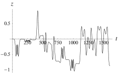
FIG. 8.: The $z$-component of the orbit shown in Fig. 3.

3 Periodic orbits

As for the four-cusp system of Dahlqvist and Russberg [17], we show that our $n=6$ example is not completely chaotic by showing numerically that there is at least one stable orbit surrounded by invariant tori (Kolmogorov–Arnol’d–Moser or KAM surfaces) which make a small region around the periodic orbit dynamically inaccessible to the chaotic orbit filling most of the energy surface.

We expect the most stable orbit to be the one with the highest symmetry allowed by the system, i.e. $2n$-fold symmetry, since this is the smoothest orbit, least like the trajectory of a billiard ball. This is illustrated in Fig. 9 for the case $n=6$, $p_{z}=0$, with the orbit passing through $(x,y)_{0}=(3,0)$. The corresponding momentum required to close the orbit is $(p_{x},p_{y})_{0}=(0,0.04925)$, giving an energy ${\mathcal{E}}=0.00170082$ and a period $28.96$. Because of its 12-fold symmetry we call this the dodecagonal orbit.

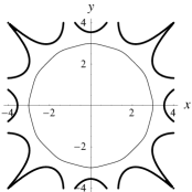
FIG. 9.: Stable periodic orbit with 12-fold symmetry — the “dodecagonal” orbit — as described in the text. The thick line shows the boundary of the energetically accessible region.

To investigate the stability of such an orbit we linearize about the orbit and calculate the eigenvalues of the matrix evolving a neighborhood of the phase-space point $(x_{0},p_{y0})$ in the $x>0$, $y=0$ half plane to its intersection with the next surface of section that is equivalent under the symmetry operation $\zeta\mapsto\exp(i\pi/6)\zeta$. [The crossing time is found numerically by searching for the first zero of $\arg\exp(-i\pi/6)\zeta(t)$.] For the case shown in Fig. 9, the eigenvalues are $-0.54162\pm 0.840624i$, which lie on the unit circle in the complex plane, indicating stability.

This stability is confirmed more graphically by the Poincaré plots in Fig. 10 for some neighboring orbits on the same energy surface as the dodecagonal orbit shown in Fig. 9. Figure 10 shows iterates of the map $(x,p_{x})\mapsto(x^{\prime},p^{\prime}_{x})$ found by calculating the crossing time $t$ with the $\theta=\pi/6$ line as described above, then calculating $x^{\prime}={\mathrm{Re}}\,\exp(-i\pi/6)\zeta(t)$, $p^{\prime}_{x}={\mathrm{Re}}\,\exp(-i\pi/6)p_{\zeta}(t)$.

Figure 10 shows an island of regular motion in a vast chaotic sea — if we start much beyond the last orbit shown, the orbit rapidly moves far away from the periodic orbit. For example, the chaotic orbit shown in the Poincaré plot, Fig. 4, started at $(x,y)_{0}=(3.02,0)$, with $p_{x}=0$ and $p_{y}$ adjusted to give the same energy as that of the periodic orbit plotted in Fig. 9.

The orbits in Fig. 10 appear to lie on invariant curves that are topologically circular, being the intersection of invariant tori with the surface of section. The quasi-triangular shape of the outer orbits is due to the existence of three unstable periodic X-points which define the separatrix between regular and chaotic motion (cf. the bifurcation with branching ratio 1/3 in Fig. 1(c) of [25]).

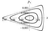
FIG. 10.: Poincaré section transverse to the dodecagonal orbit showing several satellite orbits which appear to be on invariant tori.

Scanning through a range of initial values of $x$, so as to vary the energy ${\mathcal{E}}$, we find that for all ${\mathcal{E}}$ less than the escape energy ${\mathcal{E}}_{\mathrm{esc}}$ (and somewhat beyond) the dodecagonal orbit is stable. We have not done an exhaustive study of other periodic orbits, but have established that the 4-fold-symmetric “square” orbit is unstable below an energy of about 0.1, but stabilizes above this value.

The existence of a stable periodic orbit shows that the multiple-cusp confinement system is not completely chaotic. However, the islands around the few stable orbits are very small. For instance the area occupied in the $x-p_{x}$ plane by the island shown in Fig. 10 is about $7\times 10^{-5}$, compared with the energetically accessible area of the Poincaré section, $\int[2m{\mathcal{E}}-q^{2}\psi^{2}(x,0)]^{1/2})\,dx\approx 0.37$, i.e. four orders of magnitude smaller. Even a very small amount of extrinsic stochasticity (e.g. small-angle collisions with other particles) will easily destroy such small islands of stability.

Thus we conclude that, for practical purposes, the assumption of complete chaos in the free-particle dynamics is well justified, and hence assume that any orbit covers its energy surface ergodically.

IV Wave-particle interaction model

For a given wavelength, $\lambda$, of the incident wave, the ratio $\lambda/(a/n)$ tends to infinity as $n\rightarrow\infty$. Hence we consider the long-wavelength limit, in which the wave-particle interaction is via the uniform, oscillatory electric field ${\mathbf{E}}={\mathrm{Re}}\,(\widetilde{{\mathbf{E}}}\exp i\omega t)$, where $\widetilde{{\mathbf{E}}}$ is a constant complex vector. On the other hand we assume $\omega\gg\omega_{\mathrm{p,e}}$, where $\omega_{\mathrm{p,e}}$ is the electron plasma frequency, so that the oscillatory part of the electrostatic potential can be ignored. Thus the electric field is taken to be produced by the vector potential ${\mathbf{A}}_{1}={\mathrm{Re}}\,[i(\widetilde{{\mathbf{E}}}/\omega)\exp i\omega t]$.

In reality, uniformity of ${\mathbf{E}}$ applies only during one wall-scattering event, which occurs over the scale length $a/n$, whereas ${\mathbf{E}}$ can be different at different points on the picket fence if $\lambda$ is comparable with $a$. In this paper we consider a model system in which ${\mathbf{E}}$ is strictly constant in space, but we model the real situation by choosing $\widetilde{{\mathbf{E}}}$ from a random ensemble of values with probability distribution matching the distribution of field amplitudes and phases actually encountered on the cylinder $r=a$. We also assume the distribution of initial phases to be uniform, which means that the ensemble averaging operator $\langle\cdot\rangle$ automatically includes phase averaging.

The model Hamiltonian determining the full particle dynamics is thus taken to be $H_{0}+H_{1}$, where $H_{0}$ is given by Eq. (1), and

$$H_{1}\equiv-\frac{q}{m\omega}{\mathrm{Re}}\,[i({\mathbf{p}}-q\psi{\mathbf{e}}_{z})\cdot\widetilde{{\mathbf{E}}}\exp i\omega t]\;,$$ (19)

with ${\mathbf{e}}_{z}$ being the unit vector in the $z$-direction. The above form for $H$ follows simply by expanding $({\mathbf{p}}-q{\mathbf{A}})^{2}/2m$ and dropping the term quadratic in $\widetilde{{\mathbf{E}}}$ as it has no spatial dependence and thus does not affect the dynamics. (If we had not taken ${\mathbf{E}}$ to be constant in space, it would be necessary to retain this term to include ponderomotive force effects.)

Note that $H_{1}$ produces an oscillatory correction, $\partial H_{1}/\partial{\mathbf{p}}$, to the velocity, $\dot{{\mathbf{x}}}$, that is independent of position, whereas the oscillation in $\dot{{\mathbf{p}}}$ is localized around the edge region due to the localization of $\psi$. Thus ${\mathbf{p}}$ is nonoscillatory in the middle region where $\psi$ is negligible. This is a consequence of our choice of gauge for representing ${\mathbf{E}}$, which automatically gives an oscillation-center representation [23, p. 47] in generalized momentum space. The localization of $\dot{{\mathbf{p}}}$ to the edge region where the particles are reflected is desirable since this is the region where irreversibility is introduced — in the middle region the particles simply respond adiabatically to the high-frequency field.

It is possible also to remove the oscillation in the generalized position coordinate in the middle region, so as to completely localize the interaction to the edge region, by making a canonical transformation to oscillation-center variables [26]. However, as we are interested in the diffusion in energy, not position, we have not found this transformation to be useful.

V Quasilinear diffusion

The Vlasov equation for the single-particle distribution function $f({\mathbf{x}},{\mathbf{p}},t)$ can be written

$$\partial_{t}f+\{f,H\}=0\;,$$ (20)

where the Poisson bracket $\{f,H\}\equiv\partial_{{\mathbf{x}}}f\cdot\partial_{{\mathbf{p}}}H-\partial_{{\mathbf{p}}}f\cdot\partial_{{\mathbf{x}}}H$.

We decompose $f$ into a nonfluctuating part, $\overline{f}$, and a fluctuating remainder $\widetilde{f}$. We define $\bar{f}\equiv\langle\langle f\rangle\rangle$ where $\langle\langle\cdot\rangle\rangle$ includes not only an average over the wave phase via ensemble averaging, but a phase-space average over the unperturbed energy surface: for arbitrary phase-space function $g({\mathbf{x}},{\mathbf{p}},t)$, varying on both the fast timescale $\omega^{-1}$ and a slower (diffusion) timescale, we define $\langle\langle g\rangle\rangle({\mathcal{E}},p_{z},t)$, varying only on the slow timescale, by

$$\langle\langle g\rangle\rangle\equiv\frac{1}{{\mathcal{N}}}\int_{r<a}\!\!\!d^{2}{\mathbf{x}}\int\!\!d^{2}{\mathbf{p}}\;\delta({\mathcal{E}}-H_{0}({\mathbf{x}},{\mathbf{p}}))\langle g({\mathbf{x}},{\mathbf{p}},t)\rangle\;,$$ (21)

where $r\equiv({x}^{2}+{y}^{2})^{1/2}$, $d^{2}{\mathbf{x}}\equiv dxdy$, $d^{2}{\mathbf{p}}\equiv dp_{x}dp_{y}$, $\delta$ denotes the Dirac $\delta$-function, and the normalizing factor ${\mathcal{N}}({\mathcal{E}},p_{z})$ is defined by

$${\mathcal{N}}\equiv\int_{r<a}\!\!\!d^{2}{\mathbf{x}}\int\!\!d^{2}{\mathbf{p}}\;\delta({\mathcal{E}}-H_{0}({\mathbf{x}},{\mathbf{p}}))\;.$$ (22)

The result of applying this projection operation is a function only of ${\mathcal{E}}$ and $t$, so that $\{\overline{f},H_{0}\}\equiv 0$ and hence the averaged part of the distribution function, $\overline{f}$, is invariant under the unperturbed dynamics. The projection of the distribution function onto the energy surface using the averaging operator is an extreme form of phase-space coarse-graining. Owing to the highly chaotic nature of the unperturbed dynamics we assume that this coarse-grained distribution function relaxes to a function of the constants of the unperturbed motion, ${\mathcal{E}}$ and $p_{z}$, on a timescale much faster than the quasilinear diffusion timescale. We assume all particles to be confined, so that the region of phase space defined by ${\mathcal{E}}={\mathrm{const}}$, $p_{z}={\mathrm{const}}$ is bounded within $r<a$.

Applying the operation $\langle\langle\cdot\rangle\rangle$ to Eq. (20) we have

$$\partial_{t}\overline{f}+\langle\langle\{\widetilde{f},H_{1}\}\rangle\rangle=0\;.$$ (23)

Writing the Poisson bracket in the form $\{\widetilde{f},H_{1}\}\equiv\partial_{{\mathbf{x}}}\cdot(\widetilde{f}\partial_{{\mathbf{p}}}H_{1})-\partial_{{\mathbf{p}}}\cdot(\widetilde{f}\partial_{{\mathbf{x}}}H_{1})$ and integrating by parts (assuming the particle confinement is good enough that the boundary contribution can be ignored) we find

$$\langle\langle\{\widetilde{f},H_{1}\}\rangle\rangle = \frac{1}{{\mathcal{N}}}\frac{\partial}{\partial{\mathcal{E}}}\left({\mathcal{N}}\langle\langle\,\widetilde{f}\dot{{\mathcal{E}}}\rangle\rangle\right)$$ (25)

$$\mbox{}+\frac{1}{{\mathcal{N}}}\frac{\partial}{\partial p_{z}}\left({\mathcal{N}}\langle\langle\,\widetilde{f}\dot{p}_{z}\rangle\rangle\right)\;.$$

where $\dot{{\mathcal{E}}}$ is the rate of change in the energy integral of the unperturbed system, ${\mathcal{E}}(t)\equiv H_{0}({\mathbf{x}}(t),{\mathbf{p}}(t))$, along the perturbed orbit. Noting that $\dot{H_{0}}=\{H_{0},H_{0}+H_{1}\}\equiv\{H_{0},H_{1}\}$, we see that

$$\dot{{\mathcal{E}}}=\{H_{0},H_{1}\}\;.$$ (26)

Also, $\dot{p}_{z}\equiv\{p_{z},H_{0}+H_{1}\}=\{p_{z},H_{1}\}$ [which vanishes for our simple interaction term, Eq. (19)].

Subtracting Eq. (23) from Eq. (20) we also have

$$\partial_{t}\widetilde{f}+\{\widetilde{f},H_{0}\}=-\{\overline{f},H_{1}\}+O(\widetilde{{\mathbf{E}}}^{2})\;.$$ (27)

Linearizing Eq. (27) and solving by integration along the unperturbed trajectories from an initial time $-T$, we have

$$\widetilde{f}({\mathbf{x}},{\mathbf{p}},t) = \widetilde{f}({\mathbf{x}}(-T),{\mathbf{p}}(-T),-T)$$ (30)

$$\mbox{}-\int_{-T}^{t}dt^{\prime}\;\left[\dot{{\mathcal{E}}}^{\prime}\frac{\partial{\overline{f}}}{\partial{{\mathcal{E}}}}({\mathcal{E}}^{\prime},p^{\prime}_{z},t^{\prime})\right.$$

$$\mbox{}\left.+\dot{p}^{\prime}_{z}\frac{\partial{\overline{f}}}{\partial{p_{z}}}({\mathcal{E}}^{\prime},p^{\prime}_{z},t^{\prime})\right]\;.$$

In calculating $\dot{{\mathcal{E}}}^{\prime}\equiv\dot{{\mathcal{E}}}(t^{\prime})$ using Eq. (26), the right hand side is to be evaluated at the point $({\mathbf{x}}(t^{\prime}),{\mathbf{p}}(t^{\prime}))$ on the unperturbed phase-space trajectory that passes through $({\mathbf{x}},{\mathbf{p}})$ at time $t$, and similarly for $\dot{p}_{z}(t^{\prime})$ if an interaction model is used for which it is nonvanishing.

We now observe that, for large $T$, $\widetilde{f}({\mathbf{x}}^{\prime},{\mathbf{p}}^{\prime},t^{\prime})(t^{\prime}=-T)$ becomes decorrelated from $\dot{{\mathcal{E}}}(t)$ and $\dot{p}_{z}(t)$ and thus does not contribute to the averages on the right hand side of Eq. (25). The decorrelation time is the duration of one wall-scattering event, which is of the order of the transit time

$$\tau_{\mathrm{tr}}({\mathcal{E}})\equiv\frac{a}{n|v|}$$ (31)

of a free particle with speed $|v|\equiv(2{\mathcal{E}}/m)^{1/2}$ through the scale length $a/n$ of the magnetic field variation. Thus, assuming $T\gg\tau_{\mathrm{tr}}$, we can set the initial value term $\widetilde{f}({\mathbf{x}}^{\prime},{\mathbf{p}}^{\prime},t^{\prime})(t^{\prime}=-T)$ to zero without significant error.

Also, if ${\mathbf{x}}(t)$ is in the wall-interaction region, where $\dot{{\mathcal{E}}}$ and $\dot{p}_{z}$ are significant, then ${\mathbf{x}}(-T)$ is far from the wall so $\dot{{\mathcal{E}}}(-T)$ and $\dot{p}_{z}(-T)$ are negligible (because $\psi$ is essentially zero there — see the discussion at the end of Sec. IV). Thus we can, to a very good approximation, extend the lower limit of the integral in Eq. (30) to $-\infty$.

Whereas $T$ is assumed large with respect to $\tau_{\mathrm{tr}}$, we assume it to be small with respect to the characteristic evolution time for the distribution function $\overline{f}$. (That is, we assume the wave to be of sufficiently low amplitude that it takes many wall-interaction events for significant heating to occur.) Thus we can also make the Markovian approximation that $\overline{f}({\mathcal{E}}^{\prime},p^{\prime}_{z},t^{\prime})$ can be moved outside the integral in Eq. (30) with negligible error.

Substituting Eq. (30) in Eq. (25) and then Eq. (23) we find (assuming $\dot{p}_{z}=0$) the quasilinear diffusion equation

$$\frac{\partial\overline{f}}{\partial t}=\frac{1}{{\mathcal{N}}}\frac{\partial}{\partial{\mathcal{E}}}\left({\mathcal{N}}D\frac{\partial\overline{f}}{\partial{\mathcal{E}}}\right)\;,$$ (32)

where $D({\mathcal{E}},p_{z})$ is the energy diffusion coefficient, defined by

$$D\equiv\mbox{$\frac{1}{2}$}\int_{-\infty}^{\infty}C(\tau)d\tau\;,$$ (33)

with the two-time correlation function $C({\mathcal{E}},p_{z},\tau)$

$$C(\tau)\equiv\langle\langle\dot{{\mathcal{E}}}(t-\tau)\dot{{\mathcal{E}}}(t)\rangle\rangle=\langle\langle\dot{{\mathcal{E}}}(\tau)\dot{{\mathcal{E}}}(0)\rangle\rangle\;,$$ (34)

where the second form follows from the fact that, because of the average stationarity of the dynamical system, $C$ depends only on the time difference, $\tau=t-t^{\prime}$. Also note that the projection operation $\langle\langle\cdot\rangle\rangle$, Eq. (21), can be done using either initial or final values as independent variables because the Jacobian of the transformation is unity (preservation of phase space volume) and $H_{0}$ is an invariant of the unperturbed motion. Thus $C(\tau)$ is an even function, which fact we used to extend the upper limit of the integral in Eq. (33) to infinity. We can also use time reversal invariance to show $C({\mathcal{E}},p_{z},\tau)=C({\mathcal{E}},-p_{z},-\tau)=C({\mathcal{E}},-p_{z},\tau)$.

We end this section by calculating the heating rate due to Fermi acceleration. First we define the total plasma energy per unit length in the $z$-direction,

$$U(t)\equiv\int_{0}^{\infty}d{\mathcal{E}}\int_{-\infty}^{\infty}dp_{z}\;{\mathcal{N}}{\mathcal{E}}\overline{f}\;.$$ (35)

Differentiating $U$ with respect to time, using Eq. (32) and integration by parts we find the rate of power deposition into the plasma due to reflections from the confining edge magnetic field under the influence of an electromagnetic wave

$$\dot{U}(t)=-\int_{0}^{\infty}d{\mathcal{E}}\int_{-\infty}^{\infty}dp_{z}{\mathcal{N}}D\frac{\partial\overline{f}}{\partial{\mathcal{E}}}\;.$$ (36)

We have assumed that $\partial\overline{f}/\partial{\mathcal{E}}$ vanishes at an energy less than or equal to the maximum confined energy $q^{2}\psi_{\mathrm{X}}^{2}/2m$ discussed in Sec. II C so that we can ignore boundary contributions.

VI One-dimensional model

We saw in Sec. III D 1 that most particles reflect nonadiabatically in less than one gyroperiod, and thus should not be sensitive to the details of the $y$-variation of $\psi$ (i.e. subtle resonance effects should not be important for most particles). This suggests we estimate the effect of nonadiabatic reflection by using a one-dimensional model Hamiltonian obtained by replacing $\psi(r,\theta)$ in Eq. (1) with an axisymmetric flux function, $\psi(r)$ (cf. the one-dimensional model used by Yoshida et al. [12]). The conservation of the angular momentum $p_{\theta}$ then allows formal integration of the equations of motion by the method of quadratures.

Although such a one-dimensional flux function violates Laplace’s equation, and therefore would require a plasma current to produce it, this fact is irrelevant to the single-particle dynamics. By suitable choice of $\psi(r)$ we can model the gross radial confinement properties of the two-dimensional flux function. The main loss in the physics is that $\psi(r)$ produces no radial component of ${\mathbf{B}}$, and hence no interaction with $\widetilde{E}_{\theta}$. But if we assume perfectly conducting wall boundary conditions, $\widetilde{{\mathbf{E}}}$ must be purely radial at the vacuum vessel wall (assumed just inside the array of magnetic dipoles) so $\widetilde{E}_{\theta}$ (and $\widetilde{E}_{z}$) can be assumed to be small in the interaction region anyway.

We further simplify the reflection dynamics by going to the large-$n$ limit, so that the dipoles become a linear array and we can use Cartesian coordinates as in Sec. III D 1. Also, Figs. 6 and 7 indicate that the low-energy approximation, Eq. (18), is good for nonadiabatic reflections. In this limit the field strength $B$ is independent of $y$, so we define the equivalent one-dimensional flux function $\psi(x)$ as that which gives the same field strength $B(x)$. That is, $B=|\Psi_{\mathrm{low}}^{\prime}(\xi)|\equiv\psi^{\prime}(x)$, where

$$\psi(x)=2\psi_{\mathrm{X}}\,\exp\!\left(\frac{nx}{a}\right)\;.$$ (37)

(In the above we have shifted the origin of the $x$-axis to lie on the same line as the array of dipoles.) As a final simplification of the unperturbed dynamics we evaluate $D$ only at $p_{z}=0$. That is, we consider only unperturbed orbits having the constant of the motion $p_{z}=0$.

In the large-$n$ limit the boundary region where $\psi$ is not small makes negligible contribution to Eq. (22) and thus we find the normalizing factor ${\mathcal{N}}$ to be independent of energy,

$${\mathcal{N}}=2\pi^{2}a^{2}m\;.$$ (38)

The equations of motion Eq. (12) can be integrated explicitly to give

$$x(t) = \left(\frac{a}{n}\right)\ln\left(u\,{\mathrm{sech}}\,\frac{2u(t-t_{\mathrm{max}})}{\tau_{\mathrm{X}}}\right)$$ (39)

$$p_{x}(t) = -2u\left(\frac{ma}{n\tau_{\mathrm{X}}}\right)\tanh\frac{2u(t-t_{\mathrm{max}})}{\tau_{\mathrm{X}}}$$ (40)

where $\tau_{\mathrm{X}}$ is defined in Eq. (10) and the constants of integration are $u\equiv\exp(nx_{\mathrm{max}}/a)$ and $t_{\mathrm{max}}$. Inspecting Eq. (39) we see that $x_{\mathrm{max}}$ is the maximum value of $x$ attained over the entire orbit, and $t_{\mathrm{max}}$ is the time at which this point is reached.

Assuming a perfectly conducting vacuum vessel we set $\widetilde{E}_{y}=\widetilde{E}_{z}=0$. Then, from Eq. (19), $H_{1}=-(q/m\omega){\mathrm{Re}}\,(ip_{x}\widetilde{E}_{x}\exp i\omega t)$ and we have the simple expression for the instantaneous power transfer to a particle, Eq. (26),

$$\dot{{\mathcal{E}}}=-\dot{p}_{x}\frac{\partial H_{1}}{\partial p_{x}}=\frac{q}{\omega}{\mathrm{Re}}\,\left[i\widetilde{E}_{x}\ddot{x}(t)\exp i\omega t\right]\;.$$ (41)

In evaluating the diffusion coefficient using Eq. (33), it is convenient first to commute the time integration with the averaging operation, so that we first consider the time integral of $\dot{{\mathcal{E}}}$, which gives the total energy change, $\Delta{\mathcal{E}}$, in one collision with the wall. Inserting the analytical solution Eq. (39) in Eq. (41) and integrating from $t=-\infty$ to $+\infty$, we get

$$\Delta{\mathcal{E}} = -\pi\left(\frac{a}{n}\right){\mathrm{cosech}}\left(\frac{\pi\omega\tau_{\mathrm{X}}}{4u}\right)$$ (43)

$$\mbox{}\times{\mathrm{Re}}\,\left(iq\widetilde{E}_{x}\exp i\omega t_{\mathrm{max}}\right)\;.$$

Since Eq. (40) expresses the orbit in terms of the constants of integration rather than the initial conditions, to evaluate the phase-space average we change variables from the initial conditions $x,p_{x}$ to $u$ and $s\equiv ut_{\mathrm{max}}/\tau_{\mathrm{X}}$ so $x=(a/n)\ln(u\,{\mathrm{sech}}\,2s)$, $p_{x}=2u(ma/n\tau_{\mathrm{X}})\tanh 2s$. The Jacobian of this transformation is $4(ma^{2}/n^{2}\tau_{\mathrm{X}})$, so, using Eq. (38) in Eq. (21), the phase space average over wall scattering events is transformed to

$$\langle\langle\cdot\rangle\rangle = \frac{8}{\pi}\left(\frac{ma}{n^{2}\tau_{\mathrm{X}}}\right)$$ (45)

$$\mbox{}\times\int_{-\infty}^{\infty}\frac{du\;\Theta({\mathcal{E}}-4u^{2}{\mathcal{E}}_{\mathrm{esc}})}{\sqrt{2m}\left({\mathcal{E}}-4u^{2}{\mathcal{E}}_{\mathrm{esc}}\right)^{1/2}}\int_{-\infty}^{\infty}ds\;\cdot\;,$$

where ${\mathcal{E}}_{\mathrm{esc}}$ is defined in Eq. (9) and $\Theta(\cdot)$ is the Heaviside step function.

Using Eqs. (43) and (45) in Eq. (33) we have

$$D=\frac{4}{3\pi}\frac{q^{2}\langle|\widetilde{E}_{x}|^{2}\rangle}{\omega^{2}}\frac{|v|^{3}}{a}G\left(\frac{\pi\omega\tau_{\mathrm{tr}}}{2}\right)\;,$$ (46)

where $|v|\equiv(2{\mathcal{E}}/m)^{1/2}$ is the mean velocity in the field-free region and $\tau_{\mathrm{tr}}({\mathcal{E}})$ is the transit time defined in Eq. (31). (Note that $D$ does not depend on the strength of the magnetic field in this model, only the scale length, because a change of $\psi_{\mathrm{X}}$ is equivalent simply to a shift in the origin of the $x$-axis by an amount of order $a/n$.)

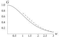
FIG. 11.: Function $G(w)$ defined in the text (solid line) and the large-$w$ asymptotic approximation (dashed line).

The function $G$ is defined as a one-dimensional integral,

$$G(w)\equiv\frac{3w^{2}}{2}\int_{0}^{1}\frac{\rho\,{\mathrm{cosech}}^{2}(w/\rho)}{(1-\rho^{2})^{1/2}}d\rho\;,$$ (47)

and is plotted as the solid line in Fig. 11. The function has been defined so as to approach unity as $w\rightarrow 0$, as discussed below in the context of the low-frequency limit, $\omega\ll 1/\tau_{\mathrm{tr}}$. The asymptotic behavior shown by the dashed line is discussed below in the context of the high-frequency limit $\omega\gg 1/\tau_{\mathrm{tr}}$.

A Low-frequency (Fermi) limit

Fermi [20] was concerned with the collision of cosmic rays with relatively slowly moving gas clouds. In our problem this corresponds to the low-frequency limit, in which a particle scatters off the magnetic field in a time much less than the period of the applied field. This makes the argument of $G$, $w=\pi\omega\tau_{\mathrm{tr}}/2$, small.

For $|w|\ll 1$, we can approximate ${\mathrm{cosech}}^{2}(w/\rho)$ in Eq. (47) by $\rho^{2}/w^{2}$ over nearly the full interval. Evaluating the integral we find $G(0)=1$.

Thus, in the low-frequency limit,

$$D=(4/3\pi)(q^{2}\langle|\widetilde{E}_{x}|^{2}\rangle/\omega^{2})(|v|^{3}/a)\;.$$ (48)

This result may be understood as the Fokker-Planck diffusion coefficient $\langle(\Delta{\mathcal{E}})^{2}\rangle/2\tau_{\mathrm{coll}}$ for particles oscillating in the applied field with the quiver velocity $\widetilde{v}$, given by

$$\widetilde{v}\equiv\frac{q\langle|\widetilde{E}_{x}|^{2}\rangle^{1/2}}{m\omega}\;,$$ (49)

giving the typical energy step at each collision with the wall $\Delta{\mathcal{E}}=m|v|\widetilde{v}$. Taking as a typical time between wall collisions $\tau_{\mathrm{coll}}=a/|v|$ we recover, to within a factor of order unity, the low-frequency energy diffusion coefficient above.

B High-frequency limit

In the high-frequency limit, the particle oscillates many times during a collision with the magnetic field and we would expect it to respond to the applied field adiabatically, gaining little energy.

For $|w|\gg 1$ the dominant contribution to the integral comes from a narrow boundary layer near $\rho=1$, in which ${\mathrm{cosech}}^{2}(w/\rho)$ may be approximated by $\exp(-2|w|)\exp(-2|w|(\rho-1))$. This gives the asymptotic behavior

$$G(w)\sim 3\sqrt{\pi}|w|^{3/2}\exp(-2|w|)\;.$$ (50)

From the dashed line in Fig. 11 we see that this asymptotic formula gives good agreement with the numerically calculated result for $|w|$ greater than about 1. We see that the energy diffusion is indeed exponentially small in this limit.

VII Discussion

In this section we give the magnetic parameters of the theory for a typical experimental device and make some observations as to the possible implications of the theory for such experiments.

Multipolar magnetic cusp confinement has become a conventional method for reducing plasma loss on the chamber walls and keeping the inner plasma volume free from magnetic field [13]. This was used in the electron-cyclotron resonance (ECR) plasma formation experiment ECRIN (ECR Ions Négatifs) [18, 19]. In ECRIN, microwave argon and hydrogen plasmas were excited in a cylindrical vessel of internal radius of about 6 cm and length 17 cm surrounded by twelve radially magnetized linear permanent magnets of alternating polarity, maximum magnetic field strength 0.2 T and microwave cw power of 100–1000 W at a frequency of 2.45 Ghz was delivered at one end of the vessel.

The primary heating occurred near the microwave input window, but it is of interest to consider whether collisionless secondary heating of free particles is possible further down the tube, which we can model by idealizing the permanent magnets as the $n=6$ linear magnetic dipole configuration used for illustration in the present paper in Figs. 1–4 and Figs. 8–10. Using $a=6$ cm gives the length unit in these figures (see Sec. II C) as $a/n=1$ cm. (In this paper we have ignored collective effects, collisions and atomic processes, all of which may be important in such experiments, so the use of the ECRIN parameters should be regarded as illustrative only.)

For ECRIN, the magnetic dipole strength was estimated to be around $K=1.5\times 10^{-5}\;\mathrm{Tm}^{2}$. Using this value in Eq. (9) gives the escape energy for electrons as ${\mathcal{E}}^{\mathrm{e}}_{\mathrm{esc}}\approx 198$ keV, and that for singly charged argon ions as ${\mathcal{E}}^{\mathrm{i}}_{\mathrm{esc}}\approx 2.7$ eV.

For electrons of energy $5$ eV the transit time, Eq. (31), is $\tau_{\mathrm{tr}}\approx 7.5$ ns, so that for the microwave heating frequency of 2.45 Ghz the argument of the transit-time reduction factor $G$ in Eq. (46) is $w\equiv\pi\omega\tau_{\mathrm{tr}}/2\approx 182$. This gives $G(w)\approx 5.5\times 10^{-155}$! Thus we see that nonresonant Fermi acceleration is clearly not an important effect in such ECR experiments. On the other hand, with $1/\tau_{\mathrm{tr}}\approx 133$ MHz, this effect can be important in rf heating experiments.

Given the strong transit-time suppression of nonresonant heating, it may be of interest to consider the resonant heating of the few free electrons penetrating deeply enough into the cusps to reach the ECR layer, and this could in principle be calculated using the quasilinear formalism developed in this paper.

However we shall content ourselves here simply with estimating the proportion of the ECR layer that is accessible to the free electrons, as opposed to the trapped electrons discussed in Sec. III C. In the neighborhood of the ECR region, Eq. (16) is satisfied only in the narrow cusp regions directed toward the magnets. We can thus Taylor expand $\psi$ to approximate this inequality by $r|\Delta\theta|\omega_{\mathrm{c}}(r)\leq 2(2m{\mathcal{E}}/m)^{1/2}$ in polar coordinates, where $\omega_{\mathrm{c}}\equiv|q|B/m$ is the electron cyclotron frequency ($=\omega$ in the ECR layer).

Summing these angular ranges over all the $2n$ cusps and dividing by $2\pi$ gives the fraction of the ECR layer accessible to free particles. Approximating $r$ by $a$ gives this fraction to be $(4/\pi)(\omega\tau_{\mathrm{tr}})^{-1}\approx 1\%$. On this basis we would expect nearly all the ECR power to be deposited in the trapped particles, with the free particles being heated through heat conduction from the trapped population and other such indirect processes.

This paper has focussed only on the effect of chaos as the source of stochasticization. In reality, particle-particle collisions may be equally or more important. Our collisionless energy diffusion coefficient will still be valid as an additive contribution to the total energy diffusion coefficient provided $\lambda_{\mathrm{mfp}}\gg a/n$, for then most particles transit the high-field edge region without suffering a collision. Elastic collisions in the central region simply provide a further stochasticization and do not affect our result provided the above inequality is satisfied. Rare collisions within the edge region would provide an independent additive mechanism for energy diffusion which might or might not dominate our collisionless mechanism depending on the ratio of transit time to the period of the applied wave.

VIII Conclusion

We have shown that, in such strongly nonaxisymmetric experiments as the multicusp geometry analyzed here, there is a strong collisionless stochasticization process due to the chaotic nature of the unperturbed particle motion. This justifies the use of the random phase approximation for successive kicks produced by coherent wave-particle interaction without having to invoke a nonlinear threshold for resonance overlap, or collisions. Such systems cannot be analyzed by area-preserving maps, and thus fall outside the general framework usually assumed for the analysis of rf and microwave heating in bounded systems [22].

As an alternative to the Fokker-Planck approach for deriving the energy diffusion equation we have developed a variant of the quasilinear diffusion formalism based on averaging the single-particle Liouville equation. This provides a general and efficient formalism for treating complex geometries.

We have applied the formalism to an exactly soluble model for nonresonant Fermi acceleration and found a transit-time correction factor that becomes exponentially small in the high-frequency limit.

Finally, we have illustrated these concepts using parameters from a fairly typical electron-cyclotron heating experiment.

REFERENCES

- [1] A. A. Vedenov, E. P. Velikhov, and R. Z. Sagdeev, Nucl. Fusion Suppl. Pt. 2, 465 (1962).
- [2] A. A. Vedenov, Plasma Phys. 5, 169 (1963).
- [3] W. E. Drummond and D. Pines, Nucl. Fusion Suppl. Pt. 3, 1049 (1962).
- [4] A. N. Kaufman, Phys. Fluids 16, 1063 (1972).
- [5] R. D. Hazeltine, S. M. Mahajan, and D. A. Hitchcock, Phys. Fluids 24, 1164 (1981).
- [6] R. V. Shurygin and R. L. Dewar, Plasma Phys. Control. Fusion 37, 1311- (1995).
- [7] T. H. Stix, Waves in Plasmas (American Institute of Physics, New York, 1992).
- [8] B. V. Chirikov, Phys. Rep. 52, 263 (1979).
- [9] J. M. Greene, J. Math. Phys. 20, 1183 (1979).
- [10] A. B. Rechester, M. N. Rosenbluth, and R. B. White, Phys. Rev. Lett. 42, 1247 (1979).
- [11] A. J. Lichtenberg and M. A. Lieberman, Regular and Chaotic dynamics, No. 38 in Applied Mathematical Sciences, 2nd ed. (Springer, New York, 1992), 1st ed. entitled Regular and Stochastic Motion (1983).
- [12] Z. Yoshida, H. Asakura, H. Kakuno, K. T. J. Morikawa, S. Takizawa, and T. Uchida, Phys. Rev. Lett. 12, 2458 (1998).
- [13] R. Burke and J. Pelletier, in Microwave Excited Plasmas, Plasma Technology, 4, edited by M. Moisan and J. Pelletier (Elsevier, Amsterdam, 1992), pp. 273–302.
- [14] M. A. Lieberman and A. J. Lichtenberg, Principles of Plasma Discharges and Materials Processing (Wiley, New York, 1994).
- [15] Y. G. Sinai, Russian Math. Surveys 25, 137 (1970), russian orig.: Usp. Mat. Nauk XXV No. 2, 141–192 (1970).
- [16] E. Ott, Chaos in dynamical systems (Cambridge Univ. Press, Cambridge, U.K., 1993).
- [17] P. Dahlqvist and G. Russberg, Phys. Rev. Lett. 65, 2837 (1990).
- [18] C. I. Ciubotariu, K. S. Golovanivsky, and M. Bacal, in ICPP96: Proc. 1996 International Conference on Plasma Physics, edited by H. Sugai and T. Hayashi (The Japan Society of Plasma Science and Nuclear Fusion Research, Nagoya, Japan, 1997), Vol. 2, p. 1238.
- [19] C.-I. Ciubotariu, D.Sc. thesis, Université Paris-Sud, 1997.
- [20] E. Fermi, Phys Rev. 75, 1169 (1949).
- [21] C. Jarzynski, Physica D 77, 276 (1994).
- [22] M. A. Lieberman and V. A. Godyak, IEEE Trans. Plasma Sci. 26, 955 (1998).
- [23] G. Schmidt, Physics of high temperature plasmas, an introduction, 1st ed. (Academic Press, New York, 1966).
- [24] P. M. Morse and H. Feshbach, Methods of Theoretical Physics (McGraw-Hill, New York, 1953).
- [25] J. M. Greene, R. S. MacKay, F. Vivaldi, and M. J. Feigenbaum, Physica D 3, 468 (1981).
- [26] R. L. Dewar, Phys. Fluids 16, 1102 (1973).
- [27] S. Wolfram, The Mathematica Book, 3rd ed. (Wolfram Media/Cambridge University Press, Champagne, Illinois, 1996).