The Construction of a Quantum Markov Partition

Abstract

We present a method for constructing a quantum Markov partition. Its elements are obtained by quantizing the characteristic function of the classical rectangles. The result is a set of quantum operators which behave asymptotically as projectors over the classical rectangles except from edge and corner effects. We investigate their spectral properties and different methods of construction. The quantum partition is shown to induce a symbolic decomposition of the quantum evolution operator. In particular, an exact expression for the traces of the propagator is obtained having the same structure as Gutzwiller periodic orbit sum.

I Introduction

For classical hyperbolic systems, symbolic dynamics provides the proper coordinates for an efficient description of the chaotic behavior [1]. Such description does not exist at the quantum level (with the exception of a few important semiclassical treatments [2]). This work is an attempt to apply the techniques of symbolic dynamics in quantum mechanics. The ultimate goal of this kind of investigations is to rewrite the equations of quantum mechanics in terms of adequate symbols for a given (chaotic) problem.

Symbolic dynamics requires a partition of phase space in various regions. We are thus faced with the problem of defining properly the quantum analogues to bounded regions of phase space. The essential difficulties for doing this are the limitations imposed by the uncertainty principle. Strictly speaking, quantum mechanics is not only in contradiction with the notion of a phase space point but also with that of a finite subset of phase space.

In a previous paper [3] a symbolic decomposition along these lines was studied, but no special constructions were necessary because the invariant manifolds were aligned with the coordinate axes, thus turning the elements of the generating partition into simple projectors. Here we generalize the method of [3] by constructing certain objects (we call them quantum rectangles) which are the quantum equivalents to the classical elements of a generating partition. Then we investigate their properties and different possibilities for their construction. The quantum rectangles behave approximately as projectors over the corresponding classical regions except from diffraction effects which are characteristic of quantum phenomena.

Once the quantum rectangles have been defined, it is straightforward to construct a quantum generating partition. In perfect analogy with the classical case, this partition leads to a symbolic decomposition of the propagator. Eventually, we obtain an exact trace formula having the same structure as Gutzwiller’s.

The rest of the paper is structured as follows. In Section II we argue that the quantum analogue of a finite region of phase space can be constructed in a natural way by simply quantizing the characteristic function of that region. In Section III we show that in the semiclassical limit the quantized regions display properties consistent with the classical ones. Section IV describes the application of the quantum generating partition to decompose the propagator. Finally, Section V contains the concluding remarks.

II Construction

The first step towards the construction of a quantum Markov partition consists in defining the quantum analogue for a finite region $R$ of the classical phase space (to be considered later as belonging to a generating partition). For the sake of simplicity, we restrict our analysis to two dimensional phase spaces with the topology of a torus (we further assume that the torus has unit area). Extensions to spaces of higher dimensionality or to other topologies can also be considered. We want to construct an operator which is the quantization of the characteristic function $\Delta_{R}$ of the region $R$,

$$\Delta_{R}(q,p)=\left\{\begin{array}[]{ll}1&\mbox{if $(q,p)\,\epsilon\,R$}\\ 0&\mbox{otherwise}\end{array}\right.\;.$$ (1)

Let us just mention two simple properties of the characteristic functions: distributivity with respect to the set intersection and normalization

$$\Delta_{R_{1}}\Delta_{R_{2}} = \Delta_{R_{1}\cap R_{2}}\;,$$ (2)

$$\int dp\,dq\,\Delta_{R}(p,q) = {\cal A}_{R}\;;$$ (3)

the integral is over the torus and ${\cal A}_{R}$ is the area (volume) of the region $R$. For the moment these regions are arbitrary but eventually they will become the elements of a partition of the phase space.

To establish the connection with quantum mechanics we make use of a phase space representation, that is, a basis $\{\widehat{B}(q_{k},p_{j}),\;1\leq k,j\leq N\}$ for operators acting on the Hilbert space $\cal H$ of dimension $N=1/2\pi\hbar$ (the $q$ and $p$ representations on the torus are discrete, and mutually related through a discrete Fourier transform [4]). Any operator $\widehat{O}$ can be written as a linear combination of the elements of the basis

$$\widehat{O}=\sum_{k,j=1}^{N}O(q_{k},p_{j})\,\widehat{B}(q_{k},p_{j})~{}.$$ (4)

Conversely, for a given symbol $O(q_{k},p_{j})$, Eq. (4) defines an operator $\widehat{O}$. We require the operator basis to decompose the identity

$$\sum_{k,j=1}^{N}\widehat{B}(q_{k},p_{j})=\openone_{\cal H}.~{}$$ (5)

Two examples of operator bases will be considered: The Kirkwood representation, associated to the basis $\{|q_{k}\rangle\langle q_{k}|p_{j}\rangle\langle p_{j}|\}$, and a representation of projectors over coherent states, $\{|q_{k}+ip_{j}\rangle\langle q_{k}+ip_{j}|\}$. In both cases the discretization used is $q_{k}=k/N$ and $p_{j}=j/N$, $1\leq k,j\leq N$, corresponding to periodic boundary conditions on the torus. We construct the coherent set starting from a circular Gaussian packet centered at $(1/2,1/2)$, say in the $q$ representation. Then, this function is evaluated in the discrete $q$ mesh and normalized. The whole set of coherent states is obtained by successive translations of the initial state to all the points $(q_{k},p_{j})$ of the mesh [4].

Both representations allow a natural construction of the quantization $\widehat{R}$ of a phase space region $R$:

$$\widehat{R}_{K} = \frac{1}{N}\sum_{k,j=1}^{N}\Delta_{R}(q_{k},p_{j})|q_{k}\rangle\langle q_{k}|p_{j}\rangle\langle p_{j}|~{},$$ (6)

$$\widehat{R}_{z} = \frac{1}{N^{2}}\sum_{k,j=1}^{N}\Delta_{R}(q_{k},p_{j})|q_{k}+ip_{j}\rangle\langle q_{k}+ip_{j}|~{}.$$ (7)

The normalization prefactors $1/N$ and $1/N^{2}$ are such that the “quantum area” (to be defined later) of the whole torus is one. The additional factor $1/N$ in the coherent case is due to the overcompleteness of that representation. While $\hat{R}_{z}$ is Hermitian and treats symmetrically $p$’s and $q$’s, $\hat{R}_{K}$ is not. Therefore, in applications we use the symmetrical combination $\widehat{R}_{K}^{s}=(\widehat{R}_{K}+\widehat{R}^{\dagger}_{K})/2$ (we come back to this point later).

By defining the operators as quantizations of the characteristic functions of the classical regions we guarantee that they have the expected semiclassical limit. We will show that the Gaussian rectangle ${R}_{z}$ tends smoothly to its classical counterpart. On the other side, the convergence of ${R}_{K}$, which has been constructed from a sharp distribution, shows characteristic rapid oscillatory structure.

III Properties

The spectral analysis of the quantum rectangles are the key to understanding their general properties. We begin by studying the Gaussian regions. For the case of a triangular region, Fig. 1 shows the way in which $\widehat{R}_{z}$ behaves in the limit $N\to\infty$. There we plot the eigenvalues $\lambda_{k}$ (associated to the eigenvectors $|\psi_{k}\rangle$) in decreasing order.

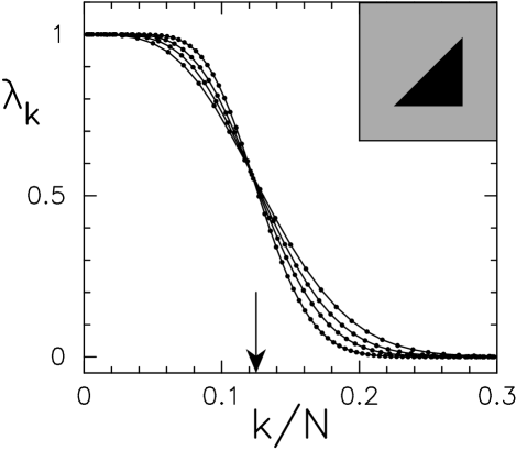
FIG. 1.: Eigenvalues of a triangular region (inset) constructed from the coherent basis. We plot the eigenvalues $\lambda_{k}$ as a function of the normalized eigenvalue number $k/N$, where $N$=$1/2\pi\hbar$ is the semiclassical parameter. We have considered $N$=90,120,160,240. Notice that as $N\to\infty$ the distribution of eigenvalues tends to a step function, the position of the step being associated with the area of the classical region (indicated with an arrow). The lines are a guide to the eye.

Most of the eigenvalues take the values $\approx 0$ or $\approx 1$. Intermediate values exist, but their relative number goes to zero in the semiclassical limit as a ratio surface to volume. Therefore, semiclassically, the rectangle behaves as a projector. Figure 2 shows that the Husimi representations $|\langle q+ip|\psi\rangle|^{2}$ of the corresponding eigenfuctions are localized on nested triangles concentrically with the boundary of the classical region.

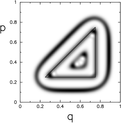
FIG. 2.: Husimi representation of three eigenfunctions of the triangular region of Fig. 1. (This is a linear gray plot, with black and white corresponding to the highest and smallest amplitudes, respectively.) The associated eigenvalues are $\lambda_{k}$=1.000,0.498,0.728; respectively $k$=4,31,90 ($N$=240). The border of the classical region is shown for reference (full black line).

The situation is very similar to that of integrable Hamiltonians, where the Husimi density of an eigenfunction is localized over the associated quantized torus and decays exponentially as one moves away from the torus. Exploiting this analogy we can derive a semiclassical quantization rule for the eigenvalues and eigenfunctions of a quantum region. Notice first that the eigenvalue equation for $\hat{R}_{z}$ is

$$\frac{1}{N^{2}}\sum_{(q,p)}\Delta_{R}|q+ip\rangle\langle q+ip|\psi_{k}\rangle=\lambda_{k}|\psi_{k}\rangle\;,$$ (8)

implying that

$$\frac{1}{N^{2}}\sum_{(q,p)\in R}|\langle q+ip|\psi_{k}\rangle|^{2}=\lambda_{k}\;$$ (9)

(the sum over the whole torus giving one). Let’s now make the following assumptions. Sums can be substituted by integrals (we are interested in the limit $N\to\infty$). The Husimi of the $k$-th eigenfunction is associated to a quantized “torus” lying at a distance $d_{k}$ from the border of the region. The function $d_{k}$ depends on the shape of the region and arises from packing $k$ quasi one-dimensional strips of area $h$ concentrically with the border of the region, starting from inside. Last, in the direction perpendicular to the torus, $\hat{y}$ ($y=0$ on the torus), the Husimi is a normalized Gaussian:

$$\exp(-y^{2}/\hbar)/\sqrt{\pi\hbar}\;.$$ (10)

Combining Eqs. (9,10) we arrive at the semiclassical quantization rule

$$\lambda_{k}=\frac{1}{2}+\frac{1}{2}\mbox{erf}\left(\frac{d_{k}}{\sqrt{\hbar}}\right)\;.$$ (11)

We give expressions for $d_{k}$ for the simplest-shaped regions: a square, the triangle of Fig. 1, and a circle

$$d_{k}=\left\{\begin{array}[]{ll}\frac{L-\sqrt{kh}}{2}&\mbox{square}\\ \frac{L-\sqrt{2kh}}{2+\sqrt{2}}&\mbox{triangle}\\ R-\sqrt{\frac{kh}{\pi}}&\mbox{circle}\end{array}\right.\;,$$ (12)

where $R$ is the radius of the circle and $L$ is the side of both the square and the triangle (see inset Fig. 3).

In Fig. 3 we compare the analytical expression (11) with the numerical results for three different regions, verifying that the agreement is excellent, even for the relatively small $N=90$.

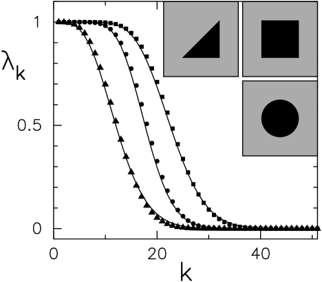
FIG. 3.: Eigenvalues of three regions: triangle, square, and circle (inset). There is a one-to-one correspondence between symbols and regions. The full lines are the analytical distributions discussed in the text ($N$=90).

The quantization of classical regions with sharp boundaries by way of coherent states presented above has the advantage of producing very smooth and analytically understandable results. The sharp edges are blurred by the Gaussian smoothing and the resulting quantum rectangles are always “soft” on the scale of $\hbar$.

Other representations, namely Kirkwood and Wigner[5], allow higher definition but display characteristic diffraction effects at the edges and corners. Fig. 4 shows the eigenvalues of the operator $\hat{R}_{K}^{s}$ of the triangular region. Notice that the distribution of eigenvalues is not smooth as in the coherent case but presents a singularity associated to boundary effects. This singularity is inherent to the sharpness of the Kirkwood construction and is also displayed by the non-hermitian rectangles $\widehat{R}_{K}$ and $\widehat{R}^{\dagger}_{K}$ (not shown). Some typical eigenfunctions are also displayed (inset). In this case, the eigenfunctions do not present the high degree of symmetry of the coherent case, but are rather irregular. The eigenvalue still determines the localization of the eigenfunction with respect to the border ($<1/2$, interior; $>1/2$, exterior).

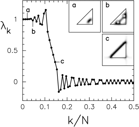
FIG. 4.: Eigenvalues of a triangular region quantized from the Kirkwood basis, and three eigenfunctions (Husimi representation, linear gray plot). The ordering of the eigenvalues is such that the parameter $|1-|\lambda_{k}||$ increases to the right. The eigenfunctions labelled a,b,c correspond to the eigenvalues $\lambda_{k}$=1.002,0.983,0.317 ($k$=3,6,18), respectively ($N$=120).

However, as the eigenfunctions are not nested like in the coherent case, the ordering is not always unambiguous.

Except for boundary effects, the Kirkwood rectangles behave asymptotically in the same way as the coherent ones, i.e., they tend to projectors over the classical regions.

Besides the nice spectral behavior discussed above, the quantum rectangles (either coherent or Kirkwood) should display some additional properties for our construction to be consistent:

(a) How does one define the “area” of a quantum region? In order to quantify the dissipation of a quantum Smale-horseshoe map, we argued in [6] that the usual operator norm $\mbox{Tr}(\hat{R}\hat{R}^{\dagger})$ is a reasonable definition of area. For the Kirkwood rectangles $\hat{R}_{K}$ it is easy to prove that this definition coincides exactly with the classical area ${\cal A}_{R}$. Alternatively one could simply define area as $\mbox{Tr}\hat{R}$, in which case classical and quantum areas are identical for both representations. Anyway, as $\hat{R}$ tends to a projector

$$\mbox{Tr}(\hat{R}\hat{R}^{\dagger})\approx\mbox{Tr}\hat{R}={\cal A}_{R}\;.$$ (13)

Thus both expressions are acceptable definitions of quantum area.

(b) For the study of spectral properties the Hermitian operator $\widehat{R}^{s}_{K}$ was preferred to the non-Hermitian $\widehat{R}_{K}$ and $\widehat{R}_{K}^{\dagger}$. The latter are more appropriate for the decomposition of the propagators we present in Section IV. However, in the limit ${\cal A}_{R}\gg\hbar$, $\widehat{R}_{K}$ and $\widehat{R}^{\dagger}_{K}$ will be approximately equal, given that they only differ in the ordering of $q$’s and $p$’s. Then $\widehat{R}_{K}$, $\widehat{R}_{K}^{\dagger}$, and $\widehat{R}_{K}^{s}$ are semiclassically equivalent.

(c) Quantization and propagation must commute: If $U$ is a classical simplectic map and $\widehat{U}$ its quantization, then

$$\widehat{U}^{T}\widehat{R}\widehat{U}^{-T}\to\widehat{U^{T}(R)}\;$$ (14)

where it is understood that one must fix $T$ and take the limit $\hbar\to 0$. To illustrate the way in which this limit may be reached we show in Fig. 5 the propagation of a Kirkwood element of the generating partition of Arnold’s cat map (see Fig. 6). Notice that besides the bulk classical propagation, diffraction effects associated to the edges and corners are clearly visible. We remark that this behavior is typical of sharp representations. Coherent rectangles behave in a much smoother way.

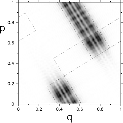
FIG. 5.: Propagation of a Kirkwood rectangle. We show a linear gray plot of $|\langle p|\hat{U}^{\dagger}\hat{R}_{1}\hat{U}|q\rangle|$, where $R_{1}$ is one of the five elements of the generating partition of Arnold’s cat map (see Fig. 6) and $\hat{U}$ is the quantized cat map (Section IV). Compare with the boundaries of the classically propagated rectangle, $U^{-1}(R_{1})$ (dots). For the sake of future referencing we also display the boundary of the element $R_{5}$ (dots). The dimension of the Hilbert space is $N$=100.

(d) We also expect quantization to commute with the classical set operations:

$$\widehat{R_{1}\cap R_{2}}\approx\widehat{R}_{1}\widehat{R}_{2}\approx\widehat{R}_{2}\widehat{R}_{1}\;,$$ (15)

$$\widehat{R_{1}\cup R_{2}}\approx\widehat{R}_{1}+\widehat{R}_{2}-\widehat{R}_{1}\widehat{R}_{2}\;.$$ (16)

In the next section we show an application of the quantum regions which is an indirect test of the validity of these statements.

IV Symbolic decomposition of the traces of the propagator

Before discussing the applications of the quantum rectangles in quantum dynamics, we present a short reminder of classical symbolic dynamics in a setting appropriate to the transition to quantum mechanics.

For a hyperbolic map $U$, symbolic dynamics relates the orbits of $U$ to symbolic sequences by means of a partition of phase space. Such partition consists of a set of regions $R_{1},R_{2},\ldots,R_{P}$ (usually called “rectangles”) which satisfy the following (Markov) properties. The boundaries of $R_{i}$ are defined by segments of the expanding and contracting manifolds of $U$. Whenever $U(R_{i})$ intersects the interior of $R_{j}$, the image cuts completely across $R_{j}$ in the unstable direction. Similarly, the backwards image $U^{-1}(R_{i})$ cuts completely across the other rectangles along the stable direction. [1, 7].

Once one has constructed the Markov partition, successively finer partitions are obtained by intersecting the elements of the basic partition with its positive and negative images by the map (product partition):

$$R_{\epsilon_{-K}\ldots\epsilon_{-1}\cdot\epsilon_{0}\epsilon_{1}\ldots\epsilon_{M}}=\bigcap_{s=-K}^{s=M}U^{s}(R_{\epsilon_{s}})\;,$$ (17)

where $\epsilon_{s}$ can take any of the values $1,2,\ldots P$. Each element of the new partition can be labeled by a different symbolic code

$$\nu(-K,M)=\epsilon_{-K}\ldots\epsilon_{-1}\cdot\epsilon_{0}\epsilon_{1}\ldots\epsilon_{M}\;.$$ (18)

As the original rectangles, the rectangles above possess the property of decomposing the phase space into disjoint regions (we do not take into account borders, which are zero-measure). When acting on these rectangles, the map is simply a shift:

$$U^{-1}(R_{\epsilon_{-K}\ldots\epsilon_{-1}\cdot\epsilon_{0}\epsilon_{1}\ldots\epsilon_{M}})=R_{\epsilon_{-K}\ldots\epsilon_{0}\cdot\epsilon_{1}\ldots\epsilon_{M}}~{}.$$ (19)

If, in the limit $K,M\to\infty$, each element of the product partition is a single point, the code is said to be complete. It may well happen that some of the intersections of Eq. (17) are empty. This means that the transitions between certain pairs of basic regions are prohibited. The information about allowed and prohibited sequences is contained in a transition matrix

$$t_{ij}=\left\{\begin{array}[]{cc}1&\mbox{if}\;f(R_{i})\cap R_{j}\neq\emptyset\\ 0&\mbox{otherwise}\end{array}\right.\;.$$ (20)

In this way one has set up a one-to-one correspondence between phase space points and allowed sequences. (The case of different sequences being associated to the same point is taken care of by identifying such sequences, and working in a quotient space.) The matrix $t_{ij}$ establishes the grammar rules that forbid certain sequences of symbols. When $t_{ij}$ is of finite size the dynamics becomes topologically conjugate to a subshift of finite type.

The existence of a symbolic dynamics allows for an exhaustive coding of the orbits of the map. In particular, periodic orbits are in correspondence with the periodic sequences of the same periodicity. Given an arbitrary system, it is a hard task to decide if it admits a symbolic dynamics; even if it does, the translation from symbols to phase space coordinates is in general extremely difficult. The example we will consider (the cat map) does not present any of these difficulties, thus eliminating non-essential complications.

In the following we show how the symbolic dynamics of a classical map can be used to decompose the traces of the quantized map. The quantum analogues of the elements of the classical generating partition are the quantum rectangles $\hat{R}$ described in Sections II and III. The quantum partitions are obtained by translating to quantum mechanics the steps in the construction of the classical ones. Starting from the quantizations of the regions of the classical basic partition, we define the quantum refinement in two steps. First the regions (quantum “projectors”) are propagated using the Heisenberg equations of motion. Then, noting that “intersections” of quantum rectangles correspond to matrix multiplications, we arrive at a quantum product partition with elements written as a time ordered multiplication of matrices

$$\hat{R}_{\nu(-K,M)} = \hat{U}^{-K}\hat{R}_{\epsilon_{-K}}\hat{U}^{K}\ldots\hat{U}^{M}\hat{R}_{\epsilon_{M}}\hat{U}^{-M}$$ (21)

$$= \hat{U}^{-K}\hat{R}_{\epsilon_{-K}}\hat{U}\hat{R}_{\epsilon_{-K+1}}\ldots\hat{R}_{\epsilon_{M-1}}\hat{U}\hat{R}_{\epsilon_{M}}\hat{U}^{-M}\;.$$ (22)

The counterpart of the classical decomposition of the phase space is the quantum decomposition of the identity

$$\sum_{\nu(-K,M)}\hat{R}_{\nu(-K,M)}=\openone/N\;,$$ (23)

$N$ being the dimension of the Hilbert space. The quantum propagation is also a shift:

$$\hat{U}^{-1}\hat{R}_{\epsilon_{-K}\ldots\epsilon_{-1}\cdot\epsilon_{0}\epsilon_{1}\ldots\epsilon_{M}}\hat{U}=\hat{R}_{\epsilon_{-K}\ldots\epsilon_{0}\cdot\epsilon_{1}\ldots\epsilon_{M}}\;.$$ (24)

Even though the quantum rectangles don’t have zero “intersection”, in the semiclassical limit, the product of two elements of the partition tends to the null operator, except from possible singularities due to border effects. Last, when $N\to\infty$ and $K,M$ fixed, the quantum rectangles tend to the classical ones. The precise meaning of this limit, and the way it is achieved were discussed in Sec. III.

The key property of the quantum partition we have constructed is the symbolic decomposition of the traces of the propagator. Consider the discrete path sum for the trace of a power of the propagator in the coherent state representation

$$\mbox{Tr}\hat{U}^{L}=\frac{1}{N^{2L}}\sum\langle\alpha_{0}|\hat{U}|\alpha_{L-1}\rangle\langle\alpha_{L-1}|\hat{U}\ldots|\alpha_{1}\rangle\langle\alpha_{1}|\hat{U}|\alpha_{0}\rangle\;$$ (25)

where the sum runs over all the closed paths $\alpha_{0},\alpha_{1},\ldots,\alpha_{L-1},\alpha_{L}\equiv\alpha_{0}$, which are discrete both in time and in the coordinates (we recall that $\alpha\equiv q+ip$ moves on the discrete $q$-$p$ grid). Semiclassically the trace of $\hat{U}^{L}$ will be dominated by the periodic trajectories (of period $L$) of the classical map $U$ and their neighboring paths. Symbolic dynamics allows for classifying not only the trajectories but also the paths according to their symbolic history. So, one has a natural way of partitioning the space of paths into disjoints subsets, each one characterized by a symbol $\nu$ of length $L$ and containing the periodic trajectory $\ldots\nu\nu\ldots$. But this mechanism of path grouping is automatically implemented by the quantum projectors:

$$\mbox{Tr}\hat{U}^{L} = \mbox{Tr}\sum_{\nu}\hat{U}\hat{R}_{\epsilon_{L-1}}\ldots\hat{U}\hat{R}_{\epsilon_{1}}\hat{U}\hat{R}_{\epsilon_{0}}$$ (26)

$$\equiv \sum_{\nu}\mbox{Tr}\hat{U}^{L}_{\nu}\;.$$ (27)

The $\hat{R}$’s are the quantum regions associated to the coherent representation and now the sum runs over the sequence labels $\nu=\epsilon_{0}\epsilon_{1}\ldots\epsilon_{L-1}$. Eq. (26) is completely equivalent to (25), the difference being just the grouping of closed paths into families sharing the same symbolic code $\nu$. Each one of these families contributes to a partial trace $\mbox{Tr}\hat{U}_{\nu}$. Analogous results are obtained in the Kirkwood case. In fact, starting from a path sum in the Kirkwood representation,

$$\mbox{Tr}\hat{U}^{L}=\frac{1}{N^{L}}\sum\langle q_{0}|p_{0}\rangle\langle p_{0}|\hat{U}\ldots\hat{U}|q_{1}\rangle\langle q_{1}|p_{1}\rangle\langle p_{1}|\hat{U}|q_{0}\rangle\;,$$ (28)

one arrives at the same result of Eq. (26) but with the Kirkwood rectangles instead of the coherent ones. Using the cyclic property, the partial traces of (26) (or the Kirkwood counterparts) can be rewritten in terms of the refined rectangles of Eq. (21)

$$\mbox{Tr}\,\hat{U}^{L}_{\nu(K,M)}=\mbox{Tr}\left[\hat{U}^{L}\hat{R}_{\nu(K,M)}\right]\;.$$ (29)

The integers $K,M$ must satisfy $K+M=L-1$, but are otherwise arbitrary. By varying $K$ and $M$ ($L$ fixed) one constructs different types of rectangles, e.g., the choice $K$=0, $M$=$L$-1 produces “unstable” rectangles (stretched along the unstable manifolds)

$$\hat{R}_{\cdot\epsilon_{0}\epsilon_{1}\ldots\epsilon_{L-1}}=\hat{R}_{\epsilon_{0}}\hat{U}^{1}\hat{R}_{\epsilon_{1}}\hat{U}^{-1}\ldots\hat{U}^{L-1}\hat{R}_{\epsilon_{L}}\hat{U}^{-(L-1)}\;.$$ (30)

Similarly, with $M=0$ and $K$=$L$-1, “stable” rectangles are obtained. Anyway, stable and unstable rectangles are related by the unitary transformation (24), ensuring that $\mbox{Tr}\hat{U}^{L}_{\nu(K,M)}$ does not depend on the particular choice of $K,M$. Moreover, the trace of each symbolic piece is cyclically invariant [as is obvious from (26)] and therefore the decompositions into invariant cycles in one-to-one correspondence with periodic orbits of the map.

The refined rectangle $\hat{R}_{\nu(K,M)}$ has as classical limit the characteristic function of the classical region $R_{\nu(K,M)}$. Thus, its role in (29) consists essentially in cutting the matrix $\hat{U}^{L}$ into pieces. The Kirkwood rectangles act onto the Kirkwood matrix $\langle p|\hat{U}^{L}|q\rangle$:

$$\mbox{Tr}\left(\hat{U}^{L}\hat{R}_{K,\nu}\right) = \sum_{q,p}\langle p|\hat{U}^{L}|q\rangle\langle q|\hat{R}_{K,\nu}|p\rangle$$ (31)

$$\approx \frac{1}{N}\sum_{q,p}\langle p|\hat{U}^{L}|q\rangle\Delta_{R_{\nu}}(q,p)\;.$$ (32)

The coherent rectangles perform a similar action but on the operator symbol $\langle\alpha|\hat{U}^{L}|\alpha\rangle$:

$$\mbox{Tr}\left(\hat{U}^{L}\hat{R}_{z,\nu}\right) \approx \mbox{Tr}\left(\hat{U}^{L}\sum_{\alpha\in R_{\nu}}|\alpha\rangle\langle\alpha|\right)$$ (33)

$$= \frac{1}{N^{2}}\sum_{\alpha}\langle\alpha|\hat{U}^{L}|\alpha\rangle\Delta_{R_{\nu}}(\alpha)\;.$$ (34)

In both cases the semiclassical partial trace is obtained by summing over that piece of the matrix which corresponds to the classical rectangle. Thus each symbolic piece captures the local structure of the propagator in the vicinity of a periodic point labeled bu $\nu$ and by stationary phase yields the Gutzwiller-Tabor contribution of the corresponding periodic orbit. Forbidden symbols lead to semiclassically small contributions[8].

The symbolic decomposition we have presented has the nice feature of reducing the problem of understanding the asymptotic limit of the traces of the propagator to the analysis of individual “partial” traces $\mbox{Tr}\hat{U}^{L}_{\nu}$, each one characterized by a code given by the symbolic dynamics, and ruled by a periodic point.

A A numerical application

The simplest system in which the quantum partitions can be applied to decompose the propagators is perhaps the baker’s map [3]. Its generating partition consists in two rectangles, which, due to the fact that the expanding and contracting directions are parallel to the coordinate axes, are solely defined by conditions on $q$. As a consequence, the quantum rectangles for the baker’s reduce exactly to projectors on subspaces [3]. This greatly simplifies the symbolic analysis of the quantum baker’s, allowing very detailed studies of its partial traces [3, 9].

However, the baker’s is too special for illustrating the properties of the rectangles: many of them are satisfied trivially. Moreover, the partial traces of the baker’s display some unpleasant anomalies that difficult the semiclassical analyses [3, 9].

Still simple enough, the Arnold’s cat map $U$ [10] is more appropriate for a general illustration of the method and can be investigated numerically. The classical cat map is defined by

$$\left(\begin{array}[]{c}q^{\prime}\\ p^{\prime}\end{array}\right)=\left(\begin{array}[]{cc}2&1\\ 1&1\end{array}\right)\left(\begin{array}[]{c}q\\ p\end{array}\right)~{}\mbox{mod 1}\;.$$ (35)

This is a linear, hyperbolic, and continuous map of the torus. As its invariant manifolds are not aligned with the coordinate axes, the rectangles of the generating partition [11] (shown in Fig. 6) are not projectors. This makes the cat map non-trivial for our purposes.

Before proceeding, we must point out that the quantum cat map presents one very particular feature: Gutwiller’s semiclassical formula gives the exact traces [12]. For this reason the cat map is not suitable for studying corrections to the trace formula. In principle, any decomposition into partial traces will introduce errors which, however, will cancel out when added up to produce the whole trace. Thus this model may be useful as a test of the mechanisms that lead to such cancellation.

Let’s now go to the details of the numerical example. The generating partition of the cat map consists of the five rectangles of Fig. 6, which, together with the “grammar rules” embodied in the transition matrix

$$t_{ij}=\left(\begin{array}[]{ccccc}01001\\ 01001\\ 10110\\ 10110\\ 10110\end{array}\right)$$ (36)

define the symbolic dynamics of the cat[11].

FIG. 6.: The five rectangles of the generating partition of Arnold’s cat map. Shown are also (parts of) the invariant manifolds of the fixed point in the origin (dashed lines), and the period two trajectory with symbolic label $\nu=51$.

For simplicity we will restrict our analysis to the decomposition of the trace of the time-two propagator

$$\mbox{Tr}\hat{U}^{2}=\sum_{\epsilon_{0},\epsilon_{1}=1}^{5}\mbox{Tr}\left(\hat{U}\hat{R}_{\epsilon_{0}}\hat{U}\hat{R}_{\epsilon_{1}}\right)\;.$$ (37)

The rectangles $\hat{R}_{\epsilon}$ are the quantum versions of the regions of Fig. 6 and can be constructed from either the coherent state representation or Kirkwood’s. The construction of the quantum propagator $\hat{U}$ for linear automorphisms of the torus is presented in [13] [notice that Arnold’s cat (35) is only quantizable for $N$ even].

Each partial trace can be written asymptotically as a Gutzwiller term plus corrections that go to zero as $N\to\infty$:

$$\mbox{Tr}\hat{U}^{2}_{\nu}=A_{\nu}\exp\left(2\pi iNS_{\nu}\right)+\delta_{\nu}(N)\;,$$ (38)

where $A_{\nu}$ is the amplitude and $S_{\nu}$ the action of the periodic orbit [14]. We remark that in the case of cat maps the corrections $\delta_{\nu}$ will cancel out exactly when summing over $\nu$ because the semiclassical trace formula is exact in this special case. In general this will not be true, and the method allows to study the corrections coming from each periodic orbit.

In order to quantify the errors associated to the symbolic partition of the space of paths, we study numerically the semiclassical limit of one element of the partition, namely $\mbox{Tr}U^{2}_{51}$. This trace is dominated by the periodic trajectory shown in Fig. 6 and its neighborhood; its asymptotic limit is the Gutzwiller formula (38) with $A_{51}=1/\sqrt{5}$ and $S_{51}=3/10$ [15].

We can understand the asymptotic behavior of the corrections $\delta_{\nu}$ by recalling that our decomposition essentially amounts to cutting the matrix of $\hat{U}$ into rectangular blocks. Let’s first estimate the corrections in the Kirkwood’s case. The Kirkwood matrix of $U^{L}$ has constant amplitude [13] and phase that oscillates rapidly except in the vicinity of the fixed points of $U^{L}$ [3]. Computing the partial trace amounts to summing up the matrix elements $\langle p|U^{2}|q\rangle$ that lie inside the region $R_{51}\equiv R_{5}\cap U^{-1}(R_{1})$ (shown in Fig. 5). In the semiclassical limit we can replace the sum by an integration and do the latter using the stationary phase method. In this approximation we must only take into account the contributions of the critical points [16]. The most important contribution comes from the the periodic orbit (critical point of the first kind) and its neighborhood. This gives rise to the Guzwiller term, which is of order zero in $\hbar$ [${\cal O}(\hbar^{0})$]. The corrections $\delta_{51}(N)$ are associated to critical points of second and third kind. The critical points of the second kind, i.e., points where the phase is stationary with respect to displacements along the borders of the rectangle, contribute with terms ${\cal O}(\hbar^{1/2})$. The corners (third kind critical points) contribute with terms ${\cal O}(\hbar^{3/2})$. (In the baker’s the situation is more complicated because of the coalescence of critical points of different kind, namely some fixed points lie on the borders of the rectangles. These anomalous points give rise to terms ${\cal O}(\log\hbar)$ [3, 9].) Having exhausted the critical points, we conclude that the border errors in Kirkwood’s representation are ${\cal O}(\hbar^{1/2})$. On the other hand, in the coherent case, one expects the amplitudes $\langle\alpha|\hat{U}^{L}|\alpha\rangle$ to decay exponentially fast as one moves away from the classical trajectory. The phases do still oscillate fast. However, due to the exponential damping, the border effects in the coherent decomposition should then be ${\cal O}[\hbar^{1/2}\exp(-C^{2}/\hbar)]$, where $C$ is proportional to the distance from the fixed point to the border. Of course, this regime will only be reached once the stationary phase neighborhood of the fixed point [whose radius is ${\cal O}(\hbar^{1/2})$] is completely contained in $R_{51}$.

For the coherent case we calculated numerically the correction $\delta_{51}$ as a function of $N$. Up to $N=100$ we computed the partial trace exactly, i.e.,

$$\frac{1}{N^{4}}\sum_{\alpha\in R_{1},\,\beta\in R_{5}}\langle\alpha|\hat{U}|\beta\rangle\langle\beta|\hat{U}|\alpha\rangle\;.$$ (39)

From then on, due to computer time limitations, we resorted to a local semiclassical approximation for the coherent-state propagator. This is equivalent to replacing the torus propagator $\langle\alpha|\hat{U}^{2}|\beta\rangle$ by a plane propagator which is the quantization of the linear dynamics in the vicinity of the period-two trajectory $\nu=51$. The errors introduced in this approximation arise from ignoring the contributions of “sources” located at equivalent (mod 1) positions in the plane [13]. These errors are also ${\cal O}[\hbar^{1/2}\exp(-C^{\prime 2}/\hbar)]$, but with $C^{\prime}$ much larger than $C$, and thus can be neglected. Once the partial trace was calculated, we obtained the correction $\delta_{\nu}$ by subtracting the Gutzwiller term.

In Fig. 7 we show the numerical results in a way that permits a direct comparison with our analytical considerations above. In fact, the log-linear plot suggests that the corrections $\delta_{\nu}$ in the coherent state decomposition are indeed exponentially small in the semiclassical parameter $1/\hbar$. Accordingly, the decomposition which uses rectangles constructed from the Kirkwood representation introduces border errors of order $\hbar^{1/2}$.

FIG. 7.: Corrections to the Gutwiller trace formula, $\nu=51$.

We recall that Gutzwiller’s trace formula is exact for the cat maps. For typical maps one expects corrections to this formula of order $\hbar^{k}$, with $k\geq 1$; e.g., $k=1$ for the perturbed cat maps [17]. Both Markov partitions considered here, either based on coherent-state or Kirkwood rectangles, allow to study such corrections term by term. In the coherent case, the partitioning of the space of paths does not introduce significant border effects, given that the contributions of neighboring paths decrease exponentially as one moves away from the central trajectory. On the other side, the use of a sharp representation like Kirkwood’s produces non-negligible boundary contributions to each partial trace. Of course these boundary terms will cancel out when the partial traces are summed up to give the whole trace. Even though, they have to be carefully identified to isolate the genuine partial corrections to the Gutzwiller trace formula.

V Concluding remarks

We have begun the application of symbolic dynamics techniques, essential in classical chaotic problems, in quantum mechanics. As a fist step we constructed quantum analogues to regions of classical phase space: they are the quantizations of the characteristic functions of the classical regions. We have used Kirkwood’s and a coherent state representation. The study of metrical and spectral properties show that they behave asymptotically as projectors over those regions. They also present the diffraction effects typical of ondulatory phenomena.

For a finite-type subshift, the quantization of the rectangles of the classical generating partition gives rise to a quantum partition which induces a symbolic decomposition of the propagator. This partition allows for writing a trace formula which is both exact and structurally identical to the Gutzwiller trace formula. Thus the problem of understanding the semiclassical limit of the traces of a propagator is reduced to the analysis of partial traces coded by the symbolic dynamics. The objects we have constructed tend asymptotically to their classical counterparts and respond to same dynamics. In this way, one can verify step by step many manipulations that up to now could only be done at a semiclassical level.

Before concluding we would like to emphasize that the construction presented here is by no means restricted to phase space regions that are Markov partitions. Any region of phase space selected for ”attention” can be handled in the same way and its quantum properties explored. For example, if a closed problem is turned into a scattering one by the removal of a section of the boundary or the attachment of a soft wave guide the decomposition leads to the consideration of coupled interior and closure problems projected from the corresponding phase space regions [18]. Another application is to think of the phase space projectors as “measurements” occurring along the quantum history of the system, and the associated decoherence that result.

- [1] R. L. Devaney, An Introduction to Chaotic Dynamical Systems, (Addison-Wesley, Redwood City, 1989).
- [2] E. B. Bogomolny, Nonlinearity 5, 805 (1992)
- [3] M. Saraceno and A. Voros, Physica D 79, 206 (1994).
- [4] M. Saraceno, Ann. Phys. (NY) 199, 37 (1990).
- [5] N. L. Balazs y B. K. Jennings, Phys. Rep. 104, 347 (1984).
- [6] M. Saraceno and R. O. Vallejos, CHAOS 6, 193 (1996).
- [7] I. P. Cornfeld, S. V. Fomin, and Ya. G. Sinai, Ergodic Theory (Springer, New York, 1982).
- [8] M. C. Gutzwiller, Chaos in Classical and Quantum Mechanics (Springer, New York, 1990).
- [9] F. Toscano, R. O. Vallejos, and M. Saraceno, Nonlinearity bf 10, 965 (1997).
- [10] V. I. Arnold y A. Avez, Ergodic Problems of Classical Mechanics (Addison–Wesley, 1989).
- [11] R. L. Adler and B. Weiss, Mem. Am. Math. Soc. 98, 1 (1970).
- [12] J. P. Keating, Nonlinearity 4, 277 (1991).
- [13] J. Hannay and M. V. Berry, Physica D 1, 267 (1980).
- [14] M. Tabor, Chaos and Integrability in Nonlinear Dynamics (Wiley, New York, 1988).
- [15] J. P. Keating, Nonlinearity 4, 309 (1991).
- [16] L. Mandel and E. Wolf, Optical coherence and quantum optics (Cambridge, New York, 1995); N. G. Van Kampen, Physica 14, 575 (1949).
- [17] P. A. Boasman and J. P. Keating, Proc. R. Soc. London Ser. A 449, 629 (1995).
- [18] A. M. Ozorio de Almeida and R. O. Vallejos (unpublished).