Noise-free Stochastic Resonance in Simple Chaotic Systems

Abstract

The phenomenon of Stochastic Resonance (SR) is reported in a completely noise-free situation, with the role of thermal noise being taken by low-dimensional chaos. A one-dimensional, piecewise linear map and a pair of coupled excitatory-inhibitory neurons are the systems used for the investigation. Both systems show a transition from symmetry-broken to symmetric chaos on varying a system parameter. In the latter state, the systems switch between the formerly disjoint attractors due to the inherent chaotic dynamics. This switching rate is found to “resonate” with the frequency of an externally applied periodic perturbation (either parametric or additive). The existence of a resonance in the response of the system is characterized in terms of the residence-time distributions. The results are an unambiguous indicator of the presence of SR-like behavior in these systems. Analytical investigations supporting the observations are also presented. The results have implications in the area of information processing in biological systems.

PACS nos.: 05.40.+j, 05.45.+b

1 Introduction

“Stochastic Resonance” (SR) is a recently observed cooperative phenomena in nonlinear systems, where the ambient noise helps in amplifying a sub threshold signal (which would have been otherwise undetected) when the signal frequency is close to a critical value [1] (see [2] for a recent review). A simple scenario for observing such a phenomena is a heavily damped bistable dynamical system (e.g., a potential well with two minima) subjected to an external periodic signal. As a result, each of the minima are alternately raised and lowered in the course of one complete cycle. If the amplitude of the forcing is less than the barrier height between the wells, the system cannot switch between the two states. However, the introduction of noise can give rise to such switching. As the noise level is gradually increased, the stochastic switchings will approach a degree of synchronization with the periodic signal until the noise is so high that the bistable structure is destroyed, thereby overwhelming the signal. So, SR can be said to occur because of noise-induced hopping between multiple stable states of a system, locking on to an externally imposed periodic signal.

The characteristic signature of SR is the non-monotonic nature of the Signal-to-Noise Ratio (SNR) as a function of the external noise intensity. A theoretical understanding of this phenomena in bistable systems, subject to both periodic and random forcing, has been obtained based on the rate equation approach [3]. As the output of a chaotic process is indistinguishable from that of a noisy system, the question of whether a similar process occurs in the former case has long been debated. In fact, Benzi et al [1] indicated that the Lorenz system of equations, a well-known paradigm of chaotic behavior might be showing SR. Later studies [4] in both discrete- and continuous-time systems seemed to support this view. However, it is difficult to guarantee that the response behavior is due to “resonance” and not due to “forcing”. In the latter case, the periodic perturbation is of so large an amplitude, that the system is forced to follow the driving frequency of the periodic forcing. The ambiguity is partly because the SNR is a monotonically decreasing function of the forcing frequency and cannot be used to distinguish between resonance and forcing.

Signature of SR can also be observed in the residence time distribution. In the presence of a periodic modulation, the distribution shows a number of peaks superposed on an exponential background. However, this is observed both in the case of resonance as well as forcing. The ambiguity is, therefore, present in theoretical [5] and experimental [6] studies of noise-free SR, where regular and chaotic phases take the role of the two stable states in conventional SR. Although the distribution of the lengths of the chaotic interval shows a multi-peaked structure, this by itself is not sufficient to ensure that the enhanced response is not due to “forcing”. In the present work this problem is avoided by measuring the response of the system in terms of the peaks in the normalized distribution of residence times [7]. For SR, the strength of the peaks shows non-monotonicity with the variation of both noise intensity and signal frequency.

In this paper we present two simple models for studying stochastic resonance where the role of noise is played by the chaos generated through the inherent dynamics of the system. In Section 2, the first model for studying deterministic SR is introduced. It is a 1-dimensional piecewise linear map with uniform slope throughout. The numerical observation of resonance in computer simulations for parametric perturbation is described and a theoretical analysis of these observations is given. Additive perturbations also give rise to similar resonance behavior. In Section 3, we consider the second model, an excitatory-inhibitory neural pair. It is additively perturbed with a very low amplitude signal and the system response is observed, for which numerical and theoretical results are given. We conclude with a discussion on the implication of such resonance phenomena for biological systems.

2 The 1-dimensional map model

Recently, SR has been studied in 1-D maps with two well-defined states (but not necessarily stable) with switching between them aided by either additive or multiplicative external noise [8]. However, dynamical contact of two chaotic 1-D maps can also induce rhythmic hopping between the two domains of the system [9]. We now show how the chaotic dynamics of a system can itself be used for resonant switching between two states, without introducing any external noise.

The model chosen here is a piecewise linear anti-symmetric map, henceforth referred to as the Discontinuous Anti-symmetric Tent (DAT) map [10], defined in the interval [$-1,1$]:

$$x_{n+1}={\rm F}(x_{n})=\left\{\begin{array}[]{ll}1+a(0.5-x_{n}),&{\rm if}~{}~{}x_{n}\geq 0.5\\ 1-a(0.5-x_{n}),&{\rm if}~{}~{}0<x_{n}<0.5\\ -1+a(0.5+x_{n}),&{\rm if}~{}~{}-0.5<x_{n}<0\\ -1-a(0.5+x_{n}),&{\rm if}~{}~{}x_{n}\leq-0.5.\end{array}\right.$$ (1)

The map has a discontinuity at $x=0$. The behavior of the system is controlled by the parameter $a$ $(0<a<4)$. The map has a symmetrical pair of fixed points $x^{*}_{1,2}=\pm{\frac{1+a/2}{1+a}}$ which are stable for $0<a<1$ and unstable for $a>1$. Another pair of unstable fixed points, $x^{*}_{3,4}=\pm{\frac{1-a/2}{1-a}}$ come into existence for $a>2$. Onset of chaos occurs at $a=1$. The chaos is symmetry-broken, i.e., the trajectory is restricted to either of the two sub-intervals R:($0,1$] and L:[$-1,0$), depending on initial condition. Symmetry is restored at $a=2$. It is to be noted that as $a\rightarrow 2$ from above, $x^{*}_{3,4}$ both collide at $x=0$ causing an interior crisis, which leads to symmetry-breaking of the chaotic attractor. The Lyapunov exponent of the map is a simple monotonic function of the parameter $a$.

To observe SR, the value of $a$ was kept close to 2, and then modulated sinusoidally with amplitude $\delta$ and frequency $\omega$, i.e.,

$$a_{n+1}=\left\{\begin{array}[]{ll}a_{0}~{}+~{}\delta~{}{\rm sin}(2\pi\omega n),&{\rm if}~{}~{}x\in{\rm R}\\ a_{0}~{}-~{}\delta~{}{\rm sin}(2\pi\omega n),&{\rm if}~{}~{}x\in{\rm L}.\end{array}\right.$$ (2)

We refer to this henceforth as multiplicative or parametric perturbation, to distinguish it from additive perturbation (discussed later).

The system immediately offers an analogy to the classical bistable well scenario of SR. The sub intervals L and R correspond to the two wells between which the system hops to and fro, aided by the inherent noise (chaos) and the external periodic forcing. The response of the system is measured in terms of the normalized distribution of residence times, $N(n)$ [7]. This distribution shows a series of peaks centered at $n_{j}=(j-{\frac{1}{2}})n_{0}$, i.e., odd-integral multiples of the forcing period, $n_{0}={\frac{1}{\omega}}$. The strength of the $j$-th peak

$$P_{j}=\int_{n_{j}-\alpha n_{0}}^{n_{j}+\alpha n_{0}}N(n)dn~{}~{}~{}(0<\alpha<0.25),$$ (3)

is obtained at different values of $\omega$, keeping $a_{0}$ fixed for $j$=1,2 and 3. To maximize sensitivity, $\alpha$ was taken to be $0.25$. For $a_{0}=2.01$ and $\delta=0.05$, the response of the system showed a non-monotonic behavior as $\omega$ was varied, with $P_{1}$ peaking at $\omega_{1}\sim 1/400$, a value dependent upon $a_{0}$ $-$ a clear signature of SR-type phenomenon. $P_{2}$ and $P_{3}$ also showed non-monotonic behavior, peaking roughly at odd-integral multiples of $\omega_{1}$ (Fig. 1 (a)).

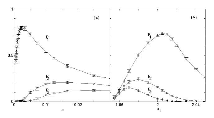
Figure 1: (a) $P_{n}$ ($n$ = 1, 2, 3) versus $\omega$ for $a_{0}=2.01$ and $\delta=0.05$, (b) $P_{n}$ ($n$ = 1, 2, 3) versus $a_{0}$ for $\omega=1/400$ and $\delta=0.05$. The circles represent the average value of $P_{n}$ for 18 different initial values of $x$, the bars representing the standard deviation.

Similar observations of $P_{j}$ were also done by varying $a_{0}$, keeping $\omega$ fixed. Fig. 1 (b) shows the results of simulations for $\omega=1/400$ and $\delta=0.05$. Here also a non-monotonicity was observed for $P_{1}$,$P_{2}$ and $P_{3}$. The broadness of the response curve and the magnitude of the peak-strengths are a function of the perturbation magnitude, $\delta$.

Analytical calculations were done to obtain the average residence-time at any one of the sub intervals. This gives the dominant time-scale of the intrinsic dynamics. Mapping the system dynamics to an approximately first-order Markov process, the mean residence time is obtained as [10]

$$<n>={\frac{-1}{{\log}({\frac{1-{\epsilon}/2-{\epsilon}^{2}/4}{1-{\epsilon}^{2}/4}})}}\simeq{\frac{-1}{\log(1-\epsilon/2)}},$$ (4)

where, $\epsilon=a_{0}-2$. So, for $a_{0}=2.01$, $<n>\simeq 200$. This predicts that a peak in the response should be observed at a frequency ${\frac{1}{2<n>}}\simeq 1/400$, which agrees with the simulation results.

The mean time spent by the trajectory in any one of the sub-intervals (L or R) can also be calculated exactly for piecewise linear maps [11]. From the geometry of the DAT map, the total fraction of R which escapes to L after $n$ iterations is found to be $l_{n}={\frac{2^{n}\epsilon}{2(2+\epsilon)^{n}}}$ [10]. This is just the probability that the trajectory spends a period of $n$ iterations in R before escaping to L ($\sum_{j=1}^{\infty}l_{j}=1$). So the average lifetime of a trajectory in R is

$$<n>=\sum_{j=1}^{\infty}(j-1)l_{j}={\frac{2}{\epsilon}}.$$ (5)

Note that, as $\epsilon\rightarrow 0$, Eqn. (4) becomes identical to the above expression. For $a_{0}$ = 2.01, $<n>$ = 200, in good agreement with the result obtained using the approximate Markov partitioning (which ensures the validity of the approximation). By symmetry of the map, identical results will be obtained if we consider the trajectory switching from L to R.

Similar study was also conducted with additive perturbation for the above map. In this case the dynamical system is defined as $x_{n+1}={\bf\rm F}(x_{n})~{}+~{}\delta{\rm sin}(2\pi\omega n)$. The simulation results showed non-monotonic behavior for the response, as either $\omega$ or $a_{0}$ was varied, keeping the other constant, but this was less marked than in the case of multiplicative perturbation.

3 The chaotic neural network model

The resonance phenomenon is also observed in an excitatory-inhibitory neural pair, with anti-symmetric, piecewise linear activation function. This type of activation function has been chosen for ease of theoretical analysis. However, sigmoidal activation functions also show similar resonance behavior.

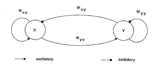
Figure 2: The pair of excitatory and inhibitory neurons used for enhancing subthreshold signal.

Fig. 2 shows a pair of coupled excitatory and inhibitory neurons. The discrete-time dynamics of such simple neural networks are found to exhibit a rich variety of behavior, including chaos [12]. If $x_{n}$ and $y_{n}$ ($x,y\in[-1,1]$) be the state of the excitatory and inhibitory elements at the $n$-th iteration, respectively, then the discrete time-evolution equation of the system is given by

$$x_{n+1}=F_{a}(w_{xx}x_{n}-w_{xy}y_{n}+I_{n}),$$

$$y_{n+1}=F_{b}(w_{yx}x_{n}-w_{yy}y_{n}+I_{n}),$$

where $w_{ij}$ is the connection weight from neuron $j$ to neuron $i$, and $I$ is an external input. The activation function is of anti-symmetric, piecewise linear nature, viz., $F_{a}(z)=-1,{\rm if}~{}z<-1/a$, $F_{a}(z)=az,{\rm if}~{}-1/a\leq z\leq 1/a$, and $F_{a}(z)=1,{\rm if}~{}z>1/a.$ Under the restriction $w_{xy}/w_{xx}=w_{yy}/w_{yx}=k$, the 2-dimensional dynamics reduces to a simple 1-dimensional form. The relevant variable is now the effective neural potential $z=x-ky$ ($z\in[-1,1]$), whose dynamics is governed by the map

$$z_{n+1}={\mathcal{F}}(z_{n})=F_{a}(z_{n})-kF_{b}(z_{n}),$$

where $a,b$ are the suitably scaled transfer function parameters. The design of the network ensures that the phase space [$-1+(kb/a),1-(kb/a)$] is divided into two well-defined and segregated sub-intervals L:[$-1+(kb/a),0$] and R:[$0,1-(kb/a)$]. The critical points of the map are at $z_{c}=\pm 1/a$. Note that, if $\mathcal{F}(z_{c})~{}(=1-\frac{kb}{a})<\mathcal{F}^{-1}(0)~{}(=\frac{1}{kb})$, the chaos is asymmetric, the trajectory being confined to any one of the subintervals. Again, if $\mathcal{F}(z_{c})>\frac{1}{b}$, the trajectory will eventually converge to a superstable periodic cycle. Therefore, for symmetric chaos, the following inequalities must be satisfied:

$$\frac{1}{kb}\leq 1-\frac{kb}{a}\leq\frac{1}{b}.$$ (6)

From the first inequality, we have $\frac{(kb)^{2}}{a}-kb+1\leq 0$, and solving for $k$ in the limiting case of an equality, the $k$-value at which the symmetry is just restored is obtained as $k=\frac{a}{2b}(1\pm\sqrt{1-\frac{4}{a}})$. Note that, real roots exist only for $a\geq 4$. Therefore, for $a<4$, there is no dynamical connection between the two sub-intervals and the trajectory, while chaotically wandering over one of the sub intervals, cannot enter the other sub interval. For $a>4$, in a certain range of $(b,k)$ values the system shows both symmetry-broken and symmetric chaos, when the trajectory visits both sub intervals in turn. The curves in $(b/a,k)$-parameter space forming a boundary between the symmetric and symmetry-broken chaotic domains are given by $k=a(1\pm\sqrt{1-(4/a)})/2b$. The second inequality of (6) gives, in the limiting case of an equality, $k=\frac{a}{b}(1-\frac{1}{b})$, which forms the boundary between the regions showing symmetric chaos and superstable periodic cycles, in the ($b/a,k$) parameter plane. The parameter space diagram in Fig. 3 shows the various dynamical regimes occurring for different values of $k$ and $b/a$, at $a=6$.

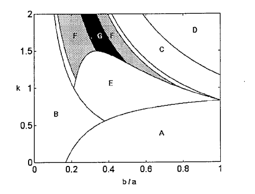
Figure 3: The ($b/a$) vs. $k$ parameter space at a = 6.0, for neural pair dynamics governed by an anti-symmetric, piecewise linear activation function. Region A: $z^{*}=1-k$ stable, B: $z^{*}=1/(1+kb)$ stable, C: $z^{*}=0$ stable, D: 2-period cycle between $[(1-k),-(1-k)]$, E: superstable periodic cycles, F: two-band symmetry-broken chaos, G: symmetric chaos. The two thin bands, between B and F, and again, between F and C, indicate regions of single-band symmetry-broken chaos.

For the simulations reported here, $a=6$ and $b=3.42$, for which the system shows symmetric chaos over a range of values of $k$.

The chaotic switching between the two sub-intervals occurs at random. However the average time spent in any of the sub-intervals before a switching event can be exactly calculated for the present model as

$$<n>=\frac{1}{bk(1-\frac{bk}{a})-1}.$$ (7)

As a complete cycle would involve the system switching from one sub-interval to the other and then switching back, the “characteristic frequency” of the chaotic process is $\omega_{c}=\frac{1}{2<n>}$. E.g., for the system to have a “characteristic frequency” of $\omega=1/400$ (say), the above relation provides the value of $k\simeq 1.3811$ for $a=6,b=3.42$. The system being symmetric, there is no net drift between L and R. However, in the presence of an external signal of amplitude $\delta$, the symmetry is broken. The net drift rate, which measures the net fraction of phase space of one sub-interval mapped to the other after one iteration, is given by $v=\delta,{\rm if}~{}~{}\delta<{\delta}_{c},$ and $v=1-(kb/a)-(1/bk),$ otherwise. The critical signal strength,

$${\delta}_{c}=1-(k^{2}b^{2}+a)/akb,$$ (8)

is a limit above which the net drift rate no longer varies in phase with the external signal. For the aforementioned system parameters $(a,b,k)$, ${\delta}_{c}\simeq 0.001$. If the input to the system is a sinusoidal signal of amplitude $\delta<{\delta}_{c}$ and frequency $\sim\omega_{c}$, we can expect the response to the signal to be enhanced, as is borne out by numerical simulations. The effect of a periodic input, $I_{n}=\delta\sin(2\pi\omega n)$, is to translate the map describing the dynamics of the neural pair, to the left and right, periodically. Fig. 4 shows the unperturbed map (solid lines) along with the maximum displacement to the left and right (dotted lines) for $\delta=0.05$.

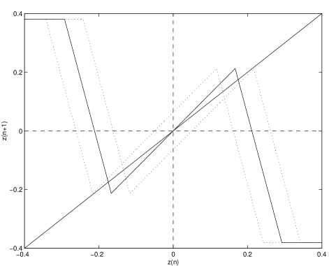
Figure 4: The map representing the dynamics of a neural pair for $a=6.0,b=3.42$ and $k=1.3811$. The figure in solid lines represent the unperturbed map ${\mathcal{F}}$, while the figures in dotted lines indicate the maximum displacement due to a periodic signal of peak amplitude, $\delta=0.05$.

The resultant intermittent switching between the two sub intervals, L and R, is shown in Fig. 5 for $\omega=1/400$ and $\delta=0.0005$.

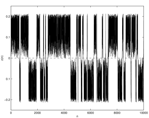
Figure 5: The time-evolution of the sinusoidally perturbed neural pair for $a=6$, $b=3.42$, $k=1.3811$, $\omega=1/400$ and $\delta=0.0005$. The broken line is the boundary between positive and negative values of $z$.

As in the previous Section, we verify the presence of resonance by looking at the peaks of the residence time distribution, where the strength of the $j$th peak is given by Eqn. (3). For maximum sensitivity, $\alpha$ is set as 0.25. As seen in Fig. 6, the dependence of $P_{j}(j=1,2,3)$ on external signal frequency, $\omega$, exhibits a characteristic non-monotonic profile, indicating the occurrence of resonance at $\omega\simeq\frac{1}{2<n>}$. For the system parameters used in the simulation, $<n>=200$. The results clearly establish that the switching between states is dominated by the sub-threshold periodic signal close to the resonant frequency.

Figure 6: The peak strengths of the normalized residence time distribution, $P_{1}$ (circles), $P_{2}$ (squares) and $P_{3}$ (diamonds), for periodic stimulation of the excitatory-inhibitory neural pair ($a=6$, $b=3.42$ and $k=1.3811$). The peak amplitude of the periodic signal is $\delta$ = 0.0005. $P_{1}$ shows a maximum at a signal frequency $\omega_{c}\simeq 1/400$. Averaging is done over 18 different initial conditions, the error bars indicating the standard deviation.

Figure 7: The strength of the first peak ($P_{1}$) in the normalized residence time distribution for periodic stimulation at $\delta=0.001$ (squares), $=0.0025$ (diamonds) and $=0.01$ (triangles). The inset shows $P_{1}$ at ${\omega}_{c}=1/400$ against $\delta$. System parameters same as in Fig. 6

.

The variation of $P_{1}$ with $\omega$ for different values of signal amplitude, $\delta$, was also studied. For $\delta>{\delta}_{c}\simeq 0.001$, the variation in the drift rate no longer matches the signal, and the maximum response is found to shift to higher frequency values (Fig. 7): e.g., at $\delta=0.01$, the maximum response in $P_{1}$ occurs at $\omega\simeq 0.03$. For $\delta<\delta_{c}$, the magnitude of $P_{1}$ at the resonance frequency, ${\omega}_{c}$, has a non-monotonic nature (Fig. 7, inset). For the system parameters mentioned here, the maximum response occurs at $\delta\sim 10^{-5}$.

These results assume significance in light of the work done on detecting SR in the biological world. In neuronal systems, a non-zero SNR is found even when the external noise is set to zero [13]. This is believed to be due to the existence of “internal noise”. This phenomenon has been examined through neural network modeling, e.g., in [14], where the main source of such “noise” is the effect of activities of adjacent neurons. The total synaptic input to a neuron, due to its excitatory and inhibitory interactions with other neurons, turns out to be aperiodic and noise-like. The neural network model employed in the present work is, however, the simplest system to date, which uses its aperiodic activity to show SR-like behavior. There is also a possible connection of such ‘resonance’ to the occurrence of epilepsy, whose principal feature is the synchronization of activity in neurons.

4 Discussion

Low-dimensional discrete-time dynamical systems are amenable to several analytical techniques and hence can be well-understood compared to other systems. The examination of resonance phenomena in this scenario was for ease of numerical and theoretical analysis. However, it is reasonable to assume that similar behavior occurs in higher-dimensional chaotic system, described by both maps and differential equations. In fact, SR has been reported for spatially extended systems (spatiotemporal SR) [15], e.g., in coupled map lattices [8]. A possible area of future work is the demonstration of phenomena analogous to spatiotemporal SR with a network of coupled excitatory-inhibitory neural pairs.

The above results indicate that deterministic chaos can play a constructive role in the processing of sub-threshold signals. It has been proposed that the sensory apparatus of several creatures use SR to enhance their sensitivity to weak external stimulus, e.g., the approach of a predator. Experimental study involving crayfish mechanoreceptor cells have provided evidence of SR in the presence of external noise and periodic stimuli [16]. The above study indicates that external noise is not necessary for such amplification as chaos in neural networks can enhance weak signals. The evidence of chaotic activity in neural processes of the crayfish [17] suggests that nonlinear resonance (as reported here) due to inherent chaos might be playing an active role in such systems. As chaotic behavior is extremely common in a recurrent network of excitatory and inhibitory neurons, such a scenario is not entirely unlikely to have occurred in the biological world. This can however be confirmed only by further biological studies and detailed modeling of the phenomena.

Acknowledgements: I would like to thank Prof. B. K. Chakrabarti for many helpful discussions and Abhishek Dhar for a careful reading of the manuscript. JNCASR is acknowledged for financial support.

References

- [1] R. Benzi, A. Sutera, and A. Vulpiani, J. Phys. A 14 (1981) L453.
- [2] L. Gammaitoni, P. Hänggi, P. Jung, and F. Marchesoni, Rev. Mod. Phys. 70 (1998) 223.
- [3] B. McNamara and K. Wiesenfeld, Phys. Rev. A 39 (1989) 4854.
- [4] G. Nicolis, C. Nicolis, and D. McKernan, J. Stat. Phys. 70 (1993) 125; V. S. Anishchenko, A. B. Neiman, and M. A. Safanova, J. Stat. Phys. 70 (1993) 183.
- [5] A. Crisanti, M. Falcioni, G. Paladin, and A. Vulpiani, J. Phys. A 27 (1994) L597.
- [6] E. Reibold, W. Just, J. Becker, and H. Benner, Phys. Rev. Lett. 78 (1997) 3101.
- [7] L. Gammaitoni, F. Marchesoni, and S. Santucci, Phys. Rev. Lett. 74 (1995) 1052.
- [8] P. M. Gade, R. Rai, and H. Singh, Phys. Rev. E 56 (1997) 2518.
- [9] C. Seko and K. Takatsuka, Phys. Rev. E 54 (1996) 956.
- [10] S. Sinha and B. K. Chakrabarti, Phys. Rev. E 58 (1998) 8009.
- [11] R. M. Everson, Phys. Lett. A 122 (1987) 471.
- [12] S. Sinha, Fundamenta Informaticae (in press, 1999); S. Sinha, Ph.D. thesis, Indian Statistical Institute, Calcutta, 1998.
- [13] K. Wiesenfeld and F. Moss, Nature 373 (1995) 33.
- [14] W. Wang and Z. D. Wang, Phys. Rev. E 55 (1997) 7379.
- [15] J. F. Lindner, B. K. Meadows, W. L. Ditto, M. E. Inchiosa, and A. R. Bulsara, Phys. Rev. Lett. 75 (1995) 3.
- [16] J. K. Douglass, L. Wilkens, E. Pantazelou, and F. Moss, Nature 365 (1993) 337.
- [17] X. Pei and F. Moss, Nature 379 (1996) 618.