Linear Parabolic Maps on the Torus
Abstract
We investigate linear parabolic maps on the torus. In a generic case these maps are non-invertible and discontinuous. Although the metric entropy of these systems is equal to zero, their dynamics is non-trivial due to folding of the image of the unit square into the torus. We study the structure of the maximal invariant set, and in a generic case we prove the sensitive dependence on the initial conditions. We study the decay of correlations and the diffusion in the corresponding system on the plane. We also demonstrate how the rationality of the real numbers defining the map influences the dynamical properties of the system.
e-mail: karol@chaos.if.uj.edu.pl tnishi@ipr.umd.edu
Corresponding author
Takashi Nishikawa
Institute for Plasma Research, University of Maryland,
College Park, MD 20742, USA
TEL +1 301 4051657, FAX +1 301 4051678, tnishi@ipr.umd.edu
PACS: 05.45.+b
Keywords: Parabolic maps on the torus, Sensitive dependence on initial conditions, Diffusion, Decay of correlations
1 Introduction
Linear area-preserving maps on the torus are often analyzed in the theory of ergodic Hamiltonian systems [1, 2]. The map , defined through
| (1) |
can be represented by the Jacobian matrix
| (2) |
Due to the area-preserving condition the matrix pertains to the non-commutative group . Let us emphasize here that the area-preserving property holds for the map when unfolded on the plane. If the dynamics takes place on the torus, folding causes overlap of some parts of the image of the unit square, so the area is not conserved.
For each matrix there exist its inverse , which defines the inverse map when the dynamics takes place on the plane . However, if the dynamics takes place on the torus (modulo restriction in Eq. (1)), one has to wrap the image of the basic square back into the torus, and some parts of this image may overlap. Consequently, some points in the torus may not have any pre-images, and the map (1) may not be invertible on the torus. On the other hand, the systems defined by matrices with all integer elements are invertible. The set of these matrices forms a discrete subgroup of . Also matrices of the type and represent invertible (but not continuous) maps on the torus for any non-integer parameters and . These matrices correspond to the horocyclic flows [1] and form two continuous subgroups of , denoted by and .
Dynamical properties of the map (1) can be characterized by the trace Tr. For the map is hyperbolic, eigenvalues of are real; and (see e.g. [5]). There exist infinitely many periodic orbits and all of them are unstable with the same stability exponent . The Arnold cat map defined by the matrix is one of the most celebrated examples of such chaotic dynamical system. Since all elements of are integer, this map is invertible on the torus (it is an automorphism on the torus). For the map is called elliptic. The eigenvalues of are complex and both Lyapunov exponents are equal to zero. Dynamics of such a system is regular and corresponds to a rotation. Properties of the elliptic maps on the torus and some features of the elliptic-hyperbolic transition were studied by Amadasi and Casartelli [3]
The intermediate case, is called parabolic. Although this case is called by Berry [5] ‘special, non-generic, set-of-measure-zero, infinitely-improbable-unless-you-deliberately-set-out-to-create-them’ case, we believe that it is worth analyzing, for two reasons. On one hand, these maps are interesting, as they lie in between the elliptic and the hyperbolic cases, which are very important for several physical applications. On the other, the parabolic maps display several remarkable properties. In particular, we show that a generic linear, area-preserving, parabolic map on the torus displays sensitivity on initial conditions. Furthermore, we demonstrate how the rationality of numbers defining the map affects the dynamics of the system. A related study of the systems leading to the interval exchange maps were discussed in [4].
This paper is organized as follows. In section 2, we discuss the general properties of parabolic maps on the torus and show corresponding families of 1D maps. In section 3 and 4, we analyze the case of rational and irrational maps, respectively. In section 5, we analyze the property of sensitive dependence on the initial conditions. Decay of correlations and the diffusion rate are analyzed in section 6.
2 Parabolic maps on the torus
If the trace of the matrix (2) fulfills , the linear map on the torus is called parabolic.111 To avoid the confusion let us mention that the 2D maps analyzed in this work are entirely different from 1D maps constructed out of parabola, also referred in the literature as parabolic maps. The corresponding dynamics is not chaotic and describes a shear flow. Since trace of a product of two matrices is usually not equal to the product of their traces, the set of all matrices with the trace equal to 2 and the determinant equal to unity (or equivalently, the set of all area-preserving, linear parabolic maps on the torus) does not possess a group structure. Apart from the matrices with integer entries and trace equal to two (such as ), the matrices belonging to the groups and also correspond to invertible parabolic maps. If both elements and of the matrix (2) are non-zero, any matrix may be represented as
| (3) |
where both the free parameters and are real. Both eigenvalues of are equal to unity, and the eigenvector reads . For parabolic maps, the two dimensional dynamics on the torus can be decomposed into a family of 1D maps, which are defined on the lines parallel to the vector . The character of the number plays therefore a special role: for rational , any line parallel to forms a closed circle on the torus, consisting of at most lines on the unit square. On the other hand, for any irrational value of , any line parallel to winds densely the entire torus.
To reduce the 2D dynamics into a family of 1D maps, let us introduce new variables defined as
| (4) |
where , and . In these variables, the map takes the following form:
where denotes the integer part of the real number . This formula is derived as following. Consider the line joining point and its image in the -plane. It crosses the horizontal discontinuities (at integer values) times, and the vertical ones times. Then the above formula is obtained from since the slope of the line is . Note that if is the initial value, the variable can be represented as with integers and , and the dynamics of can be regarded as a motion on the integer lattice . For some purposes, it is convenient to ignore the operation modulo 1 in Eq. (2), which corresponds to considering the dynamics on the -plane instead of the torus. The dynamics is described by the family of 1D maps
| (5) |
where and the initial condition is treated as a parameter. The slope of the above map is constant and equal to unity. Thus the Lyapunov exponent is equal to zero, in agreement with the assumed parabolicity of the 2D map . For rational , the map (5) is periodic with period . In the simple case , the map (5) becomes a lift of degree one, often analyzed in the theory of dynamical systems (see e.g. [6]).
3 Rational parabolic maps on the torus
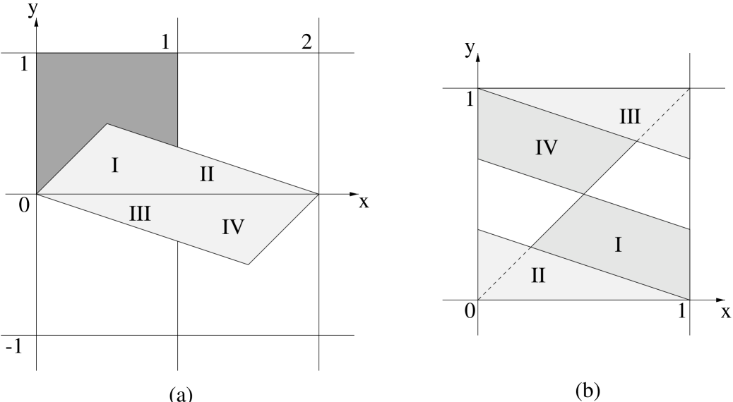
We shall call a parabolic map on the torus rational, if the parameter , which enters the matrix given by (3), is rational. If , and are rational but not integer, the corresponding map is discontinuous on all sides of the square and is not invertible on the torus. A simple example is given by and , which represents the map
| (6) |
associated to the matrix . Figure 1(a) represents the first iterate of the basic square on the plane. Due to the wrapping of this figure back into the torus, some parts of it overlap, and some fragments of the torus (denoted in white in Fig. 1(b) do not have any pre-images with respect to . Subsequent images of this set are spread over entire torus, which is what makes the dynamics of the system interesting.
Since , any trajectory originating from a single point is restricted to a circle on the torus represented by at most two parallel lines (of the same slope equal to ) in the unit square. Therefore the map does not have an attractor in the sense of attracting single trajectories. Figure 2 presents a graph obtained from ten thousand iterations of trajectories originating from ten thousand different initial points randomly chosen according to the uniform distribution on the torus. To avoid transient effects, first hundred points of each trajectory are not marked. Denote the maximal invariant set [7] (black in the figures) by
| (7) |
This set forms a support of a ‘natural’ invariant measure of the map , which may be generated by iterating the initially uniform (Lebesgue) measure by the associated Frobenius-Perron operator. The measure need not cover the set uniformly.
Remark 1. Observe the rotational symmetry of around the central point . Moreover, for any fragment of the set (black in the figure), one can find the corresponding white fragment belonging to . For example, the two large black fragments at the top and the bottom of the square form a parallelogram on the torus, which corresponds to the white parallelogram consisting of the two large white fragments on the left and on the right of the unit square. Thus there exists a symmetry in shifting the figure by vector and interchanging the colors. Therefore, the volume of the invariant set is equal to . In other words, for , the invariant set of the 1D map (5) (see Fig. 3) has volume independently of the parameter .
The fact that the invariant set contains a ball of a positive radius implies that its dimension is equal to 2. Figure 2(b) presents the magnification of the invariant set in the vicinity of the point . Note an infinite sequence of interlacing black and white parts of the figure which accumulate on the diagonal line and form some kind of self-similar structure.
Remark 2. Numerical experiments suggest that the invariant set is structurally stable. It is thus possible to get a practical approximation of the set by iterating a single trajectory of an modified system close to the analyzed map . Perturbing any of four elements of (say element by putting with a real parameter ), we get a perturbed map . Formally, this matrix does not belong to , since the area-preserving property and parabolicity, , are -violated. The perturbation couples all 1D maps together, so that by iterating one single trajectory we obtain the picture of the invariant set of the map . The numerical results show that this set approximates the set in the Hausdorff metric, while the quality of this approximation improves when decreasing the perturbation strength .
4 Irrational parabolic maps on the torus
A generic matrix belonging to contains irrational elements. To analyze such a case in some details we take the golden mean for the parameter entering the matrix (3), and set arbitrarily. This choice corresponds to the map given by
| (8) |
Due to the irrationality of the parameter , the line parallel to the eigenvector of winds densely around the entire torus. In other words, the 1D map (5) is not periodic. Thus, by iterating (almost every) single trajectory by the corresponding map given by Eq. (1), we obtain full information concerning the invariant attracting set . Such a set is shown in Fig. 4(a). Numerical analysis allows us to estimate the capacity dimension of this set and the correlation dimension . These data suggest strongly a fractal structure of the set . Note that the transformation is volume-preserving on the plane, and the existence of the attractor for this map is solely due to the modulo condition, which corresponds to wrapping the image of the unit square back on the torus.
Every irrational number can be approximated by rational numbers by truncating its expansion into the continuous fraction. For the golden mean, the consecutive approximations are given by the ratios of the adjacent Fibonacci numbers. Taking such approximations as and , we get two rational maps (3) defined by and . Estimation of the volume of the corresponding invariant sets and gives and , respectively. The volume decreases for rational maps obtained for better rational approximations of characterized by larger denominators. These results suggest that the dimensions of the sets and are equal to . However, an unusually slow convergence of the standard numerical procedure made it difficult to get a reliable numerical estimations of these dimensions. Observe similarities between and (depicted in Fig. 4(c) and (b)) and the invariant set of the irrational map presented in Fig. 4(a). Even though the sets and look similar, we conjecture that their structure is very different. Invariant set , corresponding to the rational map, is conjectured to have a non-zero volume and the capacity dimension equal to . This contrasts the properties of the set invariant under the irrational map .
5 Discontinuity and sensitivity on initial conditions
Let us denote by the boundary of the unit square. The linear, parabolic linear area-preserving map (1) is discontinuous at with probability one with respect to the Haar measure on (the only case that it is not discontinuous is when all the entries of the matrix are integer). The discontinuity can be measured by , the minimal size of the distances d and d on the torus , which depends only on the parameters of a parabolic map. It follows from the definition of that the condition is satisfied only by countable number of pairs . Thus, a generic parabolic map is characterized by a positive . The lines of discontinuity have implications for the dynamics of the system, since they split a bundle of neighboring trajectories. Similar effects were reported for elliptic maps on the torus in [9, 10].
Let us consider the set of all pre-images of the set . Although the inverse map may not exist, we define the pre-images by
| (9) |
In an analogous way, denotes the -th image of with respect to . Moreover, following [9], we define
| (10) |
Since is a countable union of sets of finite one-dimensional Lebesgue measure, it has two-dimensional Lebesgue measure zero. However, its closure may have a positive measure. Indeed that is the case for our parabolic map, and the following proposition is true.
Proposition 1. For a parabolic map with discontinuity, the set is dense in the torus and its closure has the full measure.
Proof. Let be the -ball around any point on the torus. We have to show that it must intersect with . Suppose that this -ball and all of its images do not intersect with . Due to the shearing effect of the map the diameter of grows with as
| (11) |
Therefore if is large enough, the diameter will be larger than and the image has to intersect the boundary .
Figure 5 shows the set for the irrational map defined by computed by a method similar to that used in [10], (the map is distinguished by the fact that one element of the matrix is equal to ). Proposition 1 allows us to formulate main result of the present paper concerning dynamics of a generic parabolic map.
Corollary. The dynamics generated by a generic parabolic map has sensitive dependence on initial conditions in the torus .
This property is understood as in the study of Ashwin [9] regarding elliptic discontinuous maps on the torus.
Sensitive dependence on initial conditions in a set means that for all there exists an such that for all there exists a point with and for some .
Proof. As in the proof of the Proposition 1, any -ball will intersect after some iterations. Then the next iteration will split the ball into two disjoint sets separated by , which is positive for a generic map . Hence it has sensitivity on the initial conditions.
Note that the proofs do not require that the map be irrational. It seems, however, that in the case of irrational maps, there is also another mechanism for the sensitivity due to the motion on the lines parallel to the eigenvector, whereas the rational maps do not have sensitivity along the eigenvector. Moreover, the above reasoning shows that the discontinuous parabolic maps fulfil a slightly different property of sensitive dependence introduced in the paper of Guckenheimer [12]. In any case, we emphasize that for this parabolic systems the sensitivity on initial conditions is not related with the Lyapunov exponents (which are zero in this case), but due to the discontinuity of the map.
6 Diffusion and the decay of correlations
Decay of correlations for a family of linear invertible parabolic maps on the torus was recently analyzed by Courbage and Hamdan [13]. Although these systems are not chaotic (zero Kolmogorov-Sinai entropy), the correlations decay fast. While systems with sub-exponential correlations decay are found to be generic, a class of systems with exponential decay rate was found.
Analogously, the non-invertible parabolic maps, discussed throughout this paper, display fast decay of correlations, for generic, irrational maps. Figure 6(a) presents the normalized – autocorrelation function
| (12) |
where the average is taken over initial points with respect to the natural measure. Numerical data are obtained from an ensemble of initial points chosen randomly according to the natural measure for the irrational map . The fast decay of correlations, visible in this plot, was also observed for several other initial conditions. This suggests that the autocorrelation function is independent of the initial conditions, which supports the conjecture that the dynamics is ergodic with respect to the invariant measure . As before, the fast correlation decay cannot be attributed to the positive Lyapunov exponent, but rather to discontinuity of the map .
Figure 6(b) shows the Fourier transform of the autocorrelation function in (a), which is equal to the power spectrum of the –time series. Notice the broad band continuous component in the spectrum similar to what is normally seen for chaotic maps. Also notice that there are several peaks, suggesting some periodic components both in –time series and the – autocorrelation function.
In order to discuss the diffusion process it is convenient to work with the unfolded dynamics on the plane (i.e. the operation modulo in Eq. (2) is not performed and the variable in eqn.(5) takes arbitrary real values). Diffusion coefficient may be defined as
| (13) | |||||
Since the position–position correlation function is equal to times the force–force correlation function in the direction . This function determines the diffusion rate along the axis. An argument similar to one in [11] shows
| (14) | |||||
if the above sum converges, i.e. if the correlations decay not slower than .
To study the the diffusion rate, we took initial points distributed according to the natural measure and iterated them times by a parabolic map , and computed . Figure 7 is the comparison of this and the sum of autocorrelation in (14) performed for an irrational map. Figure 8 shows the variance as a function of time for four different parabolic maps. In each case, the mean was taken over initial points. Observe two different kinds of behavior: for irrational maps, the variance is proportional to time, , which corresponds to the normal diffusion. On the other hand, for rational maps we receive , which is called ballistic diffusion. In this case, which is sometimes referred to as the anomalous diffusion, the relation (14) looses its sense: the right hand side of this equation does not converge and the limit in the definition of diffusion coefficient (13) does not exist. Examples of anomalous diffusion were reported long time ago for a particular choice of the parameters of the standard map [14], and more recently, for the kicked Harper model [15].
7 Concluding remarks
Although properties of linear area-preserving parabolic maps on the plane seem to be well understood, considering the same maps on the torus (by imposing periodic boundary conditions) makes the behavior of the system more complicated. Generically, such systems are discontinuous and non-invertible, and those properties lead to relevant dynamical implications.
For rational maps, a single trajectory is contained in a finite number of lines on the torus. This leads to the anomalous diffusion, if the associated map is considered on the plane. On the other hand, for a generic, irrational map, a typical single trajectory explores the entire maximal invariant set. The dynamics shows sensitivity on the initial conditions and the diffusion process is normal.
It is worth noting that several questions concerning the parabolic maps remain open. In particular, it would be interesting to prove the conjecture posed in this work: the volume of the maximal invariant set is a nowhere continuous function of the system parameter ; it is positive for all rational values of this parameter and zero for any irrational . Moreover, our hypothesis that the dynamics of an irrational map is ergodic with respect to the natural invariant measure is based on numerical experiments and still awaits a rigorous proof.
8 Acknowledgments
We are indebted to P. Ashwin for many valuable remarks and his constant interest in the progress of this work. We also thank M. Arjunwadkar, U. Feudel, C. Grebogi, J. Meiss, E. Ott, J. Stark, M. Wojtkowski and J. Yorke for helpful discussions and are grateful to the anonymous referee for several useful comments. K. Ż. acknowledges the Fulbright Fellowship and a support by the Polish KBN grant no. P03B 060 13.
References
- [1] I.P. Cornfeld, S.V. Fomin and Ya. G. Sinai, Ergodic Theory, Springer-Verlag, New York 1982.
- [2] R.S. MacKey and J.D. Meiss (eds.), Hamiltonian Dynamical Systems, Adam Hilger, Bristol 1987
- [3] L. Amadasi and M. Casartelli, J. Stat. Phys.65, 363 (1991).
- [4] A. Teplinsky, O. Feely, and A. Rogers, Phase-Jitter Dynamics of Digital Phase-Locked Loops, to appear in IEEE Transactions on Circuits and Systems Part I: Fundamental Theory and Applications.
- [5] M.V. Berry in [2].
- [6] A. Katok and B. Hasselblat, Introduction to Modern Theory of Dynamical Systems, Cambridge University Press, Cambridge 1995.
- [7] P. Ashwin private communication.
- [8] E. Ott, Chaos in Dynamical Systems, Cambridge University Press, Cambridge, 1994.
- [9] P. Ashwin, Non–smooth invariant circles in digital overflow oscillations, Proceedings of workshop on nonlinear Dynamics of Electronic Systems, Sevilla 1996.
- [10] P. Ashwin, Phys. Lett. A 232, 409 (1997).
- [11] J.D. Meiss, Rev. Mod. Phys. 64, 795 (1992).
- [12] J. Guckenheimer, Commun. Math. Phys. 70, 133 (1979).
- [13] M. Courbage and D. Hamdan, Ergod. Th. & Dynam. Sys. 17, 87, (1997).
- [14] C. F. F. Karney, Physica D 8, 360 (1983).
- [15] P. Leboeuf, Physica D 116, 8 (1998).