Noise-correlation-time-mediated localization in random nonlinear dynamical systems

Abstract

We investigate the behavior of the residence times density function for different nonlinear dynamical systems with limit cycle behavior and perturbed parametrically with a colored noise. We present evidence that underlying the stochastic resonancelike behavior with the noise correlation time, there is an effect of optimal localization of the system trajectories in the phase space. This phenomenon is observed in systems with different nonlinearities, suggesting a degree of universality.

By stochastic resonance (SR) it is normally understood the phenomenon by which an additive noise (usually considered uncorrelated) can enhance the coherent response of a periodically driven system. First proposed in climate model studies [1], SR was first experimentally verified by Fauve and Heslot [2], and since then this behavior has been predicted and observed in many different theoretical and experimental systems (see [3] for an extensive review and a complete list of references). In particular, the presence of SR has been discussed in a great number of models including spatio-temporal systems [4], and has helped to understand how biological organisms may use noise to enhance the transmission of weak signals through nervous systems [5, 6]. Quite recently it has been numerically shown that SR can also occur in the absence of an external periodic force as a consequence of the intrinsic dynamics of the nonlinear system [7], a behavior that has been denominated autonomous stochastic resonance. Most of the work on SR has traditionally focused on systems with additive noise, and with some exceptions (see, for instance, [8]) little attention has been given to cases where the noise perturbs the system parametrically, in spite of the well known differences with the additive situation. With respect to non-white noise, the effect of additive colored noise on SR has been considered in periodically driven overdamped systems [9], showing that the correlation time can suppress SR monotonically, a feature demonstrated experimentally in [10]. However, only very recently the situation in which the system is subject to both multiplicative and colored noise has been discussed in the literature. In [11] the authors analyze the effect of multiplicative colored noise on periodically driven linear systems, discussing the appearance of SR by changing either the intensity or the correlation time of the noise. For nonlinear models, in [12] we considered a system without periodic external force but with an intrinsic limit cycle behavior, which was parametrically perturbed by an Ornstein-Uhlenbeck (OU) noise, finding a nonmonotonic behavior of the coherence in the system response when measured as a function of the noise correlation time, while no coherence enhancement was obtained when changing the noise intensity. A similar result has also been recently obtained analytically for an overdamped linear system periodically driven and parametrically perturbed by an OU process [13].

In this paper, we present numerical evidence which suggests that underlying the SR-like behavior as a function of the noise correlation time, there is a localization effect of the system trajectories in the phase space for a particular value of the correlation time. This is obtained in systems with intrinsic limit cycle, perturbed parametrically by an OU process and with different nonlinearities, which is also a clear indication that the phenomenon is not a peculiarity of an specific model.

We study three different $2D$ random systems. The delayed regulation model, known from population dynamics [14]

$$x_{t+1}=\lambda_{t}x_{t}(1-x_{t-1}),$$ (1)

the Sel’kov model for glycolysis [15]

$$\dot{x} = -x+\lambda_{t}y+x^{2}y,$$ (2)

$$\dot{y} = b-\lambda_{t}y-x^{2}y,$$ (3)

and the Odell model also from population dynamics [16]

$$\dot{x} = x[x(1-x)-y],$$ (4)

$$\dot{y} = y(x-\lambda_{t}).$$ (5)

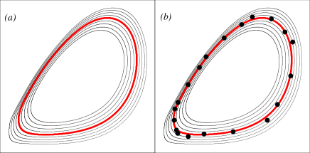
FIG. 1.: Phase space partition of Eq. (1), (a) with $N+1=9$ deterministic periodic attractors and (b) with superimposed random states (dots), and with $\sigma_{r}=0.05$ and $\tau=3$. The thick line corresponds to the attractor $\Gamma(\left\langle\lambda\right\rangle)$.

FIG. 2.: Residence times density function for (3), obtained with $50$ realizations of $5\times 10^{7}$ time steps of size $\Delta t=10^{-2}$, $\left\langle\lambda\right\rangle=0.123$, $\sigma=5\times 10^{-4}$ and $\tau=6$.

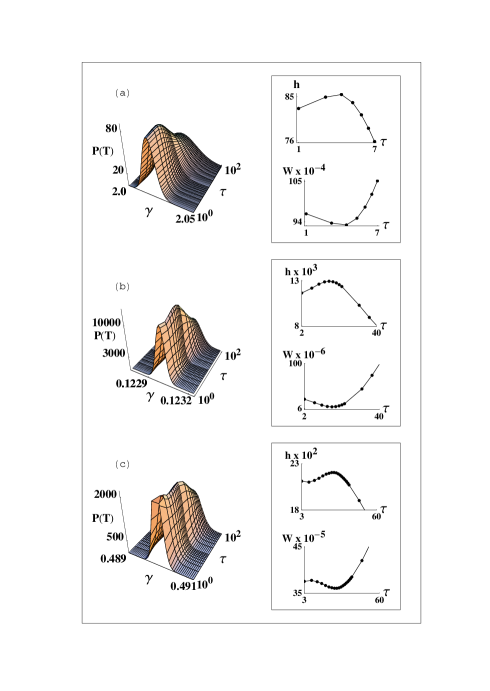
FIG. 3.: RTDF versus $\tau$ for (a) Eq. (1), (b) Eq. (3), and (c) Eq. (5). Data obtained with (a) $\left\langle\lambda\right\rangle=2.02$, $\sigma_{r}=0.05$ and 100 realizations of $10^{6}$ iterations, (b) $\left\langle\lambda\right\rangle=0.123$, $\sigma=5\times 10^{-4}$ and 50 realizations of $5\times 10^{7}$ time steps of size $\Delta t=10^{-2}$, and (c) $\left\langle\lambda\right\rangle=0.49$, $\sigma=10^{-3}$ and realizations as in (b). The inset plots indicate the height and width behavior.

Here, $t$ takes discrete values in (1) or continuous values in (3) and (5), and in all cases we will consider the control parameter as a random variable $\lambda_{t}=\lambda+\zeta_{t}$, i.e., as a deterministic part $\lambda$, plus an stochastic perturbation $\zeta_{t}$, which is assumed to be an OU process, i.e., a stationary Gaussian Markov noise with zero mean, $\left\langle\zeta_{t}\right\rangle=0$, and exponential correlation $\left\langle\zeta_{t}\zeta_{t^{\prime}}\right\rangle=\left(D/\tau\right)\exp\left(-\left|t-t^{\prime}\right|/\tau\right)$, where $\tau$ is the correlation time and $D/\tau=\sigma^{2}$ is the variance of the noise. We will refer to the square root of the variance, $\sigma$, as the intensity of the noise. The deterministic counterparts of (1), (3) and (5) undergo a supercritical Hopf bifurcation at $\lambda\equiv\lambda_{H}$ which, in the Sel’kov model, also depends on the parameter $b$.

The numerical integration has been carried out with $\lambda$ in the limit cycle parameter domain. The iteration of (1) has been recreated using an integral algorithm [17] that guarantees the quality of the correlation function in the simulations of the noise at discrete times, while (3) and (5) have been integrated by an order $2$ explicit weak scheme [18]. The results presented hereafter are independent of the initial conditions and were obtained after the decay of the initial transients.

The observed fact [12] that for a particular correlation time $\tau_{r}$ the coherence of the system oscillations has a maximum, and that the frequency of these oscillations is close to the deterministic one $w_{d}$, seems to indicate that for the resonant correlation time, the probability that the system visits the attractors associated with the mean control parameter value $\lambda=<\lambda_{t}>$ has also a maximum. If this is the case, this maximum should be accompanied with a decrease in the probability to visit other attractors associated with parameters far away from $\lambda$, or, in other words, should lead to an effect of concentration or localization of orbits around the attractor associated with $\lambda$ as soon as $\tau\sim\tau_{r}$. It is worth recalling that because of changes in the stability properties, a somehow similar localization effect can also occur in parametric deterministic systems with time dependent parameters, as is the case, for instance, in the well known parametric resonance phenomenon.

With the aim of studying the residence times distribution of the system on the different available attractors in the system periodic or quasiperiodic domain, we consider a deterministic attractor $\Lambda(\lambda)$, i.e., the attractor obtained with the deterministic counterpart of the stochastic system, evaluated at a particular value of the control parameter, $\lambda$. Next we divide the system phase space in $N+1$ attractors associated with $N+1$ values of the parameter separated a distance $\Delta\lambda$. In this way, a mesh is composed by concentric deterministic attractors centered around the stationary equilibrium state $(x^{*},y^{*})\mid_{\lambda\sim\lambda_{H}}$, with $\lambda$ in the fixed point domain. This partition looks like the one shown in Fig. 1a. With this construction, we have a series of $N+1$ attractors $\{\Lambda(\lambda_{N/2_{-}})...\Lambda(\lambda_{1_{-}}),\Lambda(\lambda_{0}),\Lambda(\lambda_{1_{+}})...\Lambda(\lambda_{N/2_{+}})\}$, where we use the definition $\lambda_{k\pm}\equiv\lambda\pm k\Delta\lambda$. This series divides the phase space in $N$ rings, each one denoted by $\Gamma(\gamma_{k})\equiv(\Lambda(\lambda_{k}),\Lambda(\lambda_{k+1}))$, where $\gamma_{k}\equiv\left(\lambda_{k+1}+\lambda_{k}\right)/2$ is the mean control parameter obtained with the control parameters that define the boundary of the ring. The stochastic system is integrated on this mesh, and its evolution describes random trajectories as the one described in Fig. 1b for the particular case of (1), visiting during a finite time each ring of the mesh. During the integration process we measure the residence time in the rings as follows: let $t_{1}^{k}$ and $t_{2}^{k}$ be the entrance and exit times to the ring $\Gamma(\gamma_{k})$, respectively. The residence time in this ring is $t(\gamma_{k})=t_{2}^{k}-t_{1}^{k}$, and we denote the residence time of the $n$ visit event to the ring $\Gamma(\gamma_{k})$ by $t_{n}(\gamma_{k})$. Then, if during an integration time $I$, which is achieved by integrating $R$ realizations of $M$ time steps, there have been $V_{k}$ visit events to the ring $\Gamma(\gamma_{k})$, the mean residence time of the system in this ring is given by the mean of the residence events, that is, $T(\Gamma(\gamma_{k}))\equiv\sum_{n=1}^{V_{k}}\frac{t_{n}(\gamma_{k})}{I}.$ Such a determination of the residence times gives an alternative statistical measure of the resonant amplification described in [12]. Therefore, given a pair $(\sigma,\tau)$, the function defined by the histogram $P(T)\equiv P(T(\gamma_{k}))\equiv P(\frac{T(\Gamma(\gamma_{k}))}{\Delta\lambda})$ is a measure of the probability density for the system state to be in the region defined by the ring $\Gamma(\gamma_{k})$ . An example of histogram is depicted in Fig. 2 and shows that the system mostly visits the attractors surrounding the ring $\Gamma(<\lambda_{t}>)$. We remark that we have carefully selected the simulation parameters to ensure that the partition does not contain overlapped attractors such that this has a well defined meaning. An illustrative example of the residence times density function (RTDF) as a function of the correlation time is depicted in Fig. 3 for the three models. Obviously, the localization of the system trajectories depends strongly on $\tau$. The RTDF height shows a nonmonotonous behavior reaching a maximum at a particular value of $\tau\sim\tau^{*}$ and, at the same value, the width $W$ calculated at the height $h/\sqrt{e}$ shows a remarkable minimum, as represented in the inset curves. The correlation time of the parametric random perturbation acts as a tuner which controls (in an statistical sense) the behavior of the system, maximizing its localization on the region of the phase space surrounding $<\lambda_{t}>$. Furthermore, the relation $h/W$ has a maximum for a particular value of $\tau$, and this optimal value depends on $\lambda=<\lambda_{t}>$, as can be appreciated in Fig.4. Such a dependence enables us to relate the optimal correlation time for maximal localization, $\tau^{*}$, with the temporal scales of the deterministic counterparts. We first study the behavior of the postponement of the bifurcation point because of the multiplicative noise in order to obtain the postponed bifurcation point $\lambda_{H}^{*}(\sigma,\tau)$.We next calculate the effective distance to the bifurcation point $\Delta\lambda^{*}=|\lambda-\lambda_{H}^{*}|$, and measure from the deterministic temporal series the period, $T^{*}$, of the oscillations when the system is evaluated at a distance $\Delta\lambda^{*}$ from the deterministic bifurcation point. With this information, in Fig. 5 we plot the behavior of $\tau^{*}$ with the quantity $\Delta T^{*}\equiv|T^{*}-T(\lambda_{H})|$, where $T(\lambda_{H})$ is the period of the deterministic system at precisely the Hopf bifurcation point. The curves can be fitted by a power law $\tau^{*}\sim\left(\Delta T^{*}\right)^{\alpha}$ with the exponents $\alpha=-0.59$, $-0.58$ and $-0.53$ for (1), (3) and (5) respectively, and this seems to indicate that the localization behavior with $\tau$ is characterized by a unique exponent with value close to $-1/2$. We note that for the case of (1) it is even possible to relate $\Delta T^{*}$ with the system implicit periodicity $T_{2}$, thus recovering a similar relation to that calculated in [12]. In this way, these results relate the resonantlike behavior previously reported in [12] using the quality factor $\beta$ [19], with an increase (in mean) of the localization of the orbits of the system.

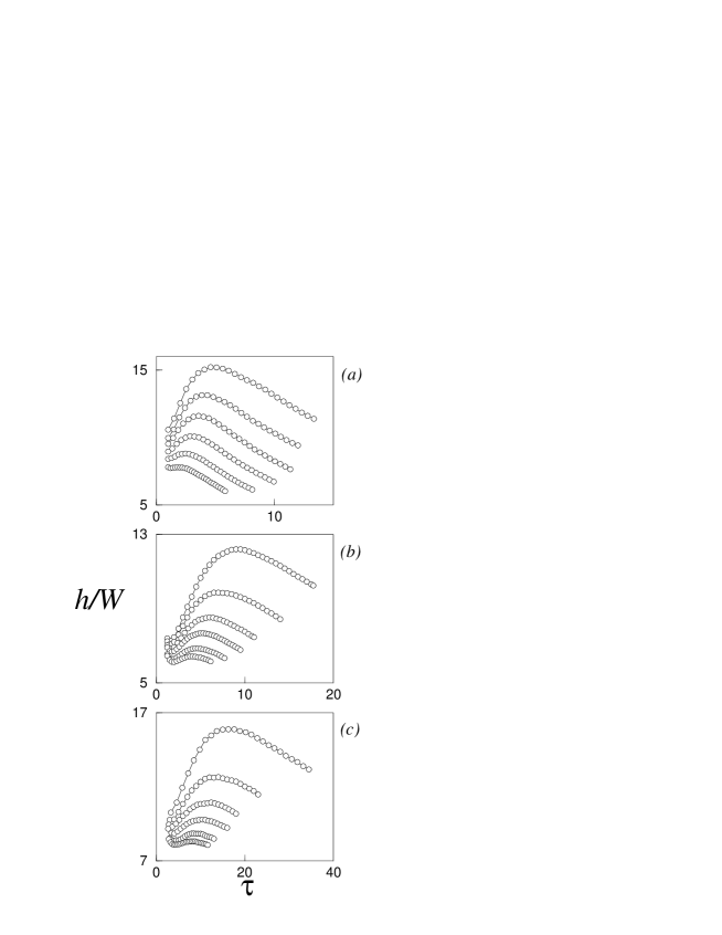
FIG. 4.: $h/W$ versus $\tau$ for different $\left\langle\lambda\right\rangle$ for (a) Eq. (1) ($h/W\times 10^{3}$, $\sigma_{r}=0.05$ and, from top to bottom $\left\langle\lambda\right\rangle=2.00828,2.01055,2.01344,2.01713,2.02182$ and $2.02781$), (b) Eq. (3) ($h/W\times 10^{6}$, $\sigma=5\times 10^{-4}$ and, $\left\langle\lambda\right\rangle=0.124,0.1235,0.123,0.1225,0.122$ and $0.1215$), and (c) Eq. (5) ($h/W\times 10^{5}$, $\sigma=10^{-3}$ and, $\left\langle\lambda\right\rangle=0.496,0.494,0.492,0.49,0.488$ and $0.486$). Number of realizations, iterations and time steps are as in Fig. 3.

From the behavior of the quantity $h/W$, it is clear that a concentration of orbits around a narrow range of bands in the phase space implies a bigger weight of those particular frequencies in the power spectrum, and, as a consequence, a nonmonotonous behavior qualitatively similar to that of Fig. 4 should be expected for $\beta$, indicating an increase of the coherence in the system response. This is indeed the case for our three models (with quality factors showing a maximum for values of the correlation time close to $\tau^{*}$) clearly indicating that the SR-like effect induced by colored noise in nonlinear systems with limit cycle behavior is quite general.

Summarizing, we have presented numerical evidence of a novel effect of enhanced localization of orbits mediated by the correlation time of a multiplicative OU process in nonlinear dynamical systems with limit cycle behavior. This effect is characterized by a power law with exponent close to $-1/2$ for all the models considered in spite of their different nonlinearities. This behavior could indicate the universal character of this phenomenon, but further research is required to clarify this point. This work also relates the SR-like behavior previously reported with this localization effect.

We acknowledge financial support from DGESEIC (Spain) project PB97-0076.

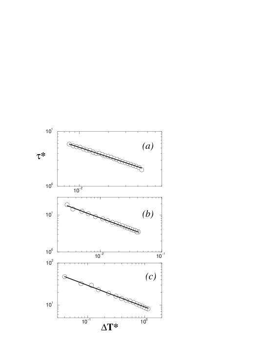
FIG. 5.: $\tau^{*}$ versus $\Delta T^{*}$ for (a) Eq. (1), (b) Eq. (3), and (c) Eq. (5). Simulation parameters are as in Fig. 3.

REFERENCES

- [1] R. Benzi, A. Sutera, and A. Vulpiani, J. Phys. A 14, L453 (1981); C. Nicolis and G. Nicolis, Tellus 33, 225 (1981).
- [2] S. Fauve and F. Heslot, Phys. Lett. 97A, 5 (1983).
- [3] L. Gammaitoni, P. Hänggi, P. Jung and F. Marchesoni, Rev. Mod. Phys. 70, 223 (1998); http: // www.pg.infn.it /sr/ biblio.html..
- [4] J. F. Lindner, B. K. Meadows, W. L. Ditto, M. E. Inchiosa and A. R. Bulsara, Phys. Rev. Lett., 75, 3 (1995).
- [5] J. Douglass, L. Wilkens, E. Pantazelou, and F. Moss, Nature 365, 337 (1993).
- [6] B. J. Gluckman, T. I. Netoff, E. J. Neel, W. L. Ditto, M. L. Spano and S. J. Schiff, Phys. Rev. Lett. 77, 4098 (1996).
- [7] H. Gang, T. Ditzinger, C. Z. Ning, and H. Haken, Phys. Rev. Lett. 71, 807 (1993).
- [8] L. Gammaitoni, F. Marchesoni, E. Menichella-Saetta and S. Santuci, Phys. Rev. E 49, 4878 (1994).
- [9] L. Gammaitoni, E. Menichella-Saetta, S. Santucci, F. Marchesoni and C. Presilla, Phys. Rev. A 40, 2114 (1989); P. Hänggi, P. Jung, C. Zerbe and F. Moss, J. Stat. Phys. 70, 25 (1993).
- [10] R. N. Mantegna and B. Spagnolo, Nuovo Cimento D 17, 873 (1995).
- [11] A. Fulinski, Phys. Rev. E 52, 4523 (1995); V. Berdichevsky and M. Gitterman, Europhys. Lett. 36, 161 (1996).
- [12] J. L. Cabrera and F. J. de la Rubia, Europhys. Lett. 39, 123 (1997).
- [13] A. V. Barzykin, K. Seki and F. Shibata, Phys. Rev. E 57, 6555 (1998).
- [14] J. Maynard Smith, Mathematical Ideas in Biology (Cambridge University Press, Cambridge, 1968); J. R. Pounder and T. D. Rogers, Bull. Math. Biol. 42, 551 (1980).
- [15] E. E. Sel’kov, Eur. J. Biochem. 4, 79 (1968).
- [16] G. M. Odell, in: L. A. Segel (ed.), Mathematical Models in Molecular and Cellular Biology (Cambridge University Press, Cambridge, 1980).
- [17] R. F. Fox, I. R. Gatland, R. Roy, and G. Vemury, Phys. Rev. A 38, 5938 (1988).
- [18] P. E. Kloeden and E. Platen, Numerical Solution of Stochastic Differential Equations (Springer-Verlag, Berlin, 1992).
- [19] The quality factor , as defined in [7], is an useful quantity to measure the changes in the degree of coherence of an autonomous system and subject to noise. For these systems the principal peak in the power spectrum has a finite height and width, and, therefore, any variation in the system response (indicating a change in the coherence) leads to changes either in the height, the width or in both. The quality factor is a good indicator incorporating both quantities.