Cross-spectral analysis of physiological
tremor and muscle activity.
I. Theory and application to unsynchronized EMG

J. Timmer¹, M. Lauk^1,2, W. Pfleger¹ and G. Deuschl³

¹Zentrum für Datenanalyse und Modellbildung, Eckerstr. 1, 79104 Freiburg, Germany

²Neurologische Universitätsklinik Freiburg, Breisacher Str. 64, 79110 Freiburg, Germany

³Neurologische Universitätsklinik Kiel, Niemannsweg 147, 24105 Kiel, Germany

(to appear in Biological Cybernetics)

We investigate the relationship between the extensor electromyogram (EMG) and tremor time series in physiological hand tremor by cross-spectral analysis. Special attention is directed to the phase spectrum and the effects of observational noise. We calculate the theoretical phase spectrum for a second order linear stochastic process and compare the results to measured tremor data recorded from subjects who did not show a synchronized EMG activity in the corresponding extensor muscle. The results show that physiological tremor is well described by the proposed model and that the measured EMG represents a Newtonian force by which the muscle acts on the hand.

1 Introduction

Time series of hand tremor and the related muscle activities of the flexor and extensor muscles are obtained by measuring the acceleration of the hand (denoted here by ACC) and the surface electromyogram (denoted here by EMG). The ACC data of physiological tremor have been described as a linear stochastic process driven by uncorrelated firing motoneurons (Stiles and Randall 1967; Randall 1973; Rietz and Stiles 1974; Elble and Koller 1990; Gantert et al. 1992; Timmer et al. 1993). The description of physiological tremor by a linear model is reasonable because linear approximations hold due to its small amplitude. These linear stochastic processes and their spectral and cross-spectral properties were studied exhaustively (Bloomfield 1976; Brockwell and Davis 1987; Priestley 1989). Usually, they are denoted by autoregressive processes, since actual values are given by a linear combination of past values plus a driving noise. In terms of physics, these processes are linear damped oscillators driven by noise.

In the context of linear stochastic processes the relation between two processes can be analyzed by investigating phase and modulus, i.e. coherency, of the normalized cross-spectrum. Applications of cross-spectral analysis to EMG and ACC data of physiological tremor are reported in (Fox and Randall 1970; Pashda and Stein 1973; Elble and Randall 1976; Stiles 1983; Iaizzo and Pozos 1992). Up to now, the coherency and the phase spectrum were investigated only at a single frequency. In particular, the phase was always interpreted as a time delay between the two processes.

The interpretation of the phase spectrum as a whole is difficult. For example, as will be shown below, the phase spectrum between EMG and ACC time series depends only on the mechanical properties of the hand and does not allow to draw conclusions on the dynamics of the driving force, i.e. the EMG. In general, the phase spectrum can only be interpreted under quite strong assumptions about the interrelation of the processes. We discuss those cases relevant for the EMG – ACC relationship. Finally, we compare the spectra predicted from the model with those estimated from measured data.

The paper is organized as follows: In the next section we briefly describe the data. In Section 3 we introduce the mathematical background for this and a companion paper (Timmer et al. 1998). Section 4 gives theoretical and empirical results for physiological tremors showing a flat EMG power spectrum, resulting from unsynchronized muscle activity. EMG power spectra exhibiting a synchronization and the possible role of reflexes are discussed in a companion paper (Timmer et al. 1998).

2 The data

The data were recorded from normal subjects. The recording technique is described in detail elsewhere (Deuschl et al. 1991). Briefly, the time series of the hand tremor (ACC) were measured by a light-weight piezo-resistive accelerometer. The sampling rate is 300 Hz. The outstretched hand is supported at the wrist. We recorded three data sets for each subject, the first with the hand unloaded, the second with a 500gr load and the third with a 1000gr load. The weights were fixed on the belly of the outstretched hand. External elements as the amplifiers and the piezoresistive sensors produce additive white observational noise in each recorded time series, uncorrelated to the measured dynamical process itself. The variance of the observational noise can be estimated from the high frequency part of the power spectrum where the contribution of the tremor oscillation can be neglected. This noise contributes up to 10% of the variance of the recorded data and has a significant effect on the estimated coherency and phase spectra as will be shown in Section 3.

The EMG time series (EMG) were measured by surface electrodes fixed over the belly of the extensor carpi ulnaris muscle and the flexor carpi ulnaris muscle. These data represent broad band noise. The information about a possible synchronization of the muscle activity is encoded in a modulation of this noise. The data were high pass filtered (cut-off frequency 80 Hz) in order to remove movement artifacts, rectified in order to obtain time series reflecting the muscle activity (Journee 1983) and then low pass filtered (cut-off frequency 150 Hz) to avoid aliasing. Finally, the signals were digitized and fed into a computer for off-line analysis.

Like the tremor time series the EMG time series are contaminated with additive observational noise. Its variance cannot be estimated analogously to that of the ACC data, since uncorrelated EMG activity also shows a flat power spectrum at higher frequencies indistinguishable from that of the observational noise.

Time series from 58 subjects who showed no significant EMG synchronization, i.e. a flat spectrum, were examined. The statistical decision of consistency with a flat spectrum was performed by means of a Kolmogorov-Smirnov test at the level of confidence p=0.05 (Timmer et al. 1996). A representative example of such a time series is shown in Fig. 1. Time series from 19 subjects with enhanced physiological tremor who showed a significant EMG synchronization are analyzed in the companion paper. In each time series the mean was subtracted and all series were scaled to variance one.

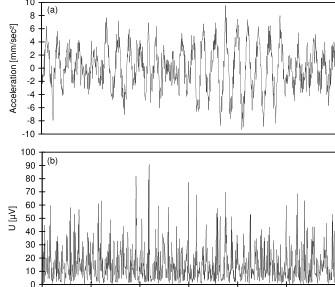
Figure 1: Acceleration of the hand (a) and rectified EMG (b) of physiological tremor.

3 Mathematical methods

In this section we introduce the mathematical methods that will be used in following sections and the companion paper to analyze the simulated and the measured data. Firstly, we briefly summarize the time and frequency domain properties of linear stochastic processes before discussing the cross-spectral estimation and interpretation. Special attention will be payed to the effects of observational noise which is always present in the data of physiological tremor and its EMG and renders the interpretation of the mathematical results more difficult.

3.1 Linear stochastic processes

An example of a linear stochastic process is the autoregressive (AR) process of order $p$ :

$$x(t)=\sum_{i=1}^{p}a_{i}\,x(t-i)\,+\,\epsilon(t)\quad,$$ (1)

where $\epsilon(t)$ denotes uncorrelated Gaussian noise with variance $\sigma^{2}$. For ease of notation we set the sampling interval to unity for the theoretical discussions. Such a process can be interpreted in terms of physics as a combination of relaxators and damped oscillators (Honerkamp 1993). For example, an AR process of order 2 with appropriate parameters $a_{1}$ and $a_{2}$ describes from a physical standpoint a linear, damped oscillator with characteristic period $T$ or frequency $\omega=1/T$, and relaxation time $\tau$. $T$ and $\tau$ are related to the parameters $a_{1}$ and $a_{2}$ by:

$$a_{1} = 2\cos\left(\frac{2\pi}{T}\right)\,\exp\,(-1/\tau)$$ (2)

$$a_{2} = -\exp\,(-2/\tau)\qquad.$$ (3)

AR processes can be generalized to the autoregressive moving average (ARMA) processes by including past driving noise terms in the dynamics. A more substantial generalization is the linear state space model (Honerkamp 1993). It allows one to model explicitly the observational noise $\eta(t)$ that covers the dynamical variable $\vec{x}(t)$ which is mapped to the observation by $C$ and contributes to the measured $z(t)$:

$$\vec{x}(t) = A\,\vec{x}(t-1)+\vec{\epsilon}(t)$$ (4)

$$z(t) = C\,\vec{x}(t)+\eta(t)\qquad.$$ (5)

This model has been applied successfully to physiological tremor time series (Gantert et al. 1992). If the observational noise is not modeled explicitly, e.g. by applying an ARMA model, the characteristic times will be underestimated and statistical tests to decide on the model order will fail to detect the correct order (König and Timmer 1997). This might explain the high model order reported earlier (Randall 1973; Miao and Sakamoto 1995).

3.2 Spectral properties of linear stochastic processes

The power spectrum $\mbox{S}(\omega)$ of a mean zero and unit variance process $x(t)$ is defined as the Fourier transform of the autocorrelation function $\mbox{ACF}(\tau)$ :

$$\mbox{ACF}(\tau) = <x(t)\,x(t-\tau)>$$ (6)

$$\mbox{S}(\omega) = \frac{1}{2\pi}\sum_{\tau}\mbox{ACF}(\tau)e^{-i\omega\tau}\,,\omega\in[-\pi,\pi]$$ (7)

with ”$<\,>$” denoting expectations. The estimation of the power spectrum is usually based on the Fourier transform $\mbox{F}(\omega)$ and the periodogram $\mbox{Per}(\omega)$ of the data :

$$X(\omega) = \frac{1}{\sqrt{N}}\sum_{t=1}^{N}x(t)\,\exp\,(-i\,\omega\,t)$$ (8)

$$\mbox{Per}(\omega) = |\,X(\omega)\,|^{2}$$ (9)

and is evaluated at the frequencies:

$$\omega_{k}=\frac{2\pi k}{N},\quad k=-\frac{N}{2},\ldots,\frac{N}{2}-1\quad.$$ (10)

The expectation of the periodogram is the power spectrum but the periodogram is not a consistent estimator for the power spectrum since the standard deviation of this $\chi^{2}_{2}$ distributed random variable is equal to its mean and does not decrease with increasing number of data (Brockwell and Davis 1987; Priestley 1989):

$$\mbox{Per}(\omega)\sim\frac{1}{2}\mbox{S}(\omega)\chi^{2}_{2}\quad.$$ (11)

In order to estimate the power spectrum, the periodogram has to be convolved by a window function $W(j)$ of width $2h+1$ :

$$\widehat{\mbox{S}}(\omega_{k})=\frac{1}{2\pi}\sum_{j=-h}^{h}W(j)\,\mbox{Per}(\omega_{k+j})\quad.$$ (12)

It is also possible to estimate the power spectrum by averaging the periodograms of segments of the data or by fitting an AR process to the data and calculate the spectrum of the fitted process. General aspects of spectral estimation as well as confidence intervals are given in (Brockwell and Davis 1987; Priestley 1989). Special aspects concerning spectral estimation for tremor time series are discussed in (Timmer et al. 1996).

For linear processes the power spectrum can be calculated analytically. In the case of an AR process of order 2 it is given by:

$$\mbox{S}(\omega)=\frac{1}{2\pi}\frac{\sigma^{2}}{|1-a_{1}\exp(-i\omega)-a_{2}\exp(-2i\omega)|^{2}}\quad.$$ (13)

Expressed in terms of $T$ and $\tau$, the power spectrum shows for $|\cos(2\pi/T)|\cosh(1/\tau)\leq 1$ a peak at the frequency:

$$\omega_{peak}=\arccos\left(\cos(2\pi/T)\,\cosh(1/\tau)\right)\quad.$$ (14)

Therefore, for small $\tau$, the peak of the power spectrum is not located at the frequency $2\pi/T$. The width of the peak is proportional to $1/\tau$. If the driving force is characterized by some nontrivial power spectrum $\mbox{S}_{drive}(\omega)$ instead of the constant spectrum of uncorrelated white noise (13) changes to:

$$\mbox{S}(\omega)=\frac{\mbox{S}_{drive}(\omega)}{|1-a_{1}\exp(-i\omega)-a_{2}\exp(-2i\omega)|^{2}}\quad.$$ (15)

3.3 Cross-spectral analysis

Analogously to the univariate quantities introduced in the previous section the cross-spectrum $\mbox{CS}(\omega)$ of two zero mean and unit variance time series $x(t)$ and $y(t)$ is defined as the Fourier transform of cross-correlation function $\mbox{CCF}(\tau)$ :

$$\mbox{CCF}(\tau) = <x(t)\,y(t-\tau)>$$ (16)

$$\mbox{CS}(\omega) = \frac{1}{2\pi}\sum_{\tau}\mbox{CCF}(\tau)\exp(-i\,\omega\,\tau)$$

$$= <X(\omega)\,Y^{\ast}(\omega)>\quad.$$

Here ^∗ denotes complex conjugation. The coherency spectrum $\mbox{Coh}(\omega)$ is defined as the modulus of the normalized cross-spectrum $\mbox{CS}(\omega)$ :

$$\mbox{Coh}(\omega)=\frac{|\mbox{CS}(\omega)|}{\sqrt{S_{x}(\omega)S_{y}(\omega)}}\quad$$ (18)

and the phase spectrum $\Phi(\omega)$ by the representation:

$$\mbox{CS}(\omega)=|\mbox{CS}(\omega)|\,\exp(i\,\Phi(\omega))\quad.$$ (19)

It can be shown that $\mbox{Coh}(\omega)$ equals one whenever $y(t)$ is a linear function of $x(t)$. This holds especially for the coherency between an AR process and its driving noise $\epsilon(t)$ (Brockwell and Davis 1987; Priestley 1989). Thus, the coherency can be interpreted as a measure of linear predictability. The interpretation of the phase spectrum is more difficult. For the following cases the phase spectrum can be calculated analytically :

• If the process $y(t)$ is a time delayed version of process $x(t)$, i.e. $y(t)=x(t-\Delta t)$, the phase spectrum is given by a straight line with its slope determined by $\Delta t$ :

  $$\Phi(\omega)=\Delta t\,\omega\quad.$$ (20)

• If $y(t)$ is the derivative of $x(t)$, i.e. $y(t)=\dot{x}(t)$ a constant phase spectrum of $-\frac{\pi}{2}$ results.

  $$\Phi(\omega)=-\pi/2\quad.$$ (21)

• In the case of an AR process of order 2 (AR[2]), the phase spectrum between the driving noise $\epsilon(t)$ and the resulting process is given by :

  $$\Phi(\omega)=\mbox{arctan}\left(\frac{a_{1}\sin{\omega}+a_{2}\sin{2\omega}}{1-a_{1}\cos{\omega}-a_{2}\cos{2\omega}}\right)\quad.$$ (22)

  It is important to note that the phase spectrum does not change if the driving noise is not a Gaussian white noise process. Because of the linearity of the system, eq. (22) holds whenever the driving process shows a broad band power spectrum. It might even be chaotic. If the relaxation time $\tau$ is not smaller than the period $T$, the phase relation $\Phi_{discr}(\omega)$ between an (time-discrete) AR[2] process and its driving noise (22) is in good approximation related to the well known phase relation $\Phi_{cont}(\omega)$ for a (time-continuous) differential equation of a linear, driven damped oscillator by:

  $$\Phi_{cont}(\omega)\cong\Phi_{discr}(\omega)+\omega\quad.$$ (23)

  Eq. (23) shows that there is a substantial difference between a discrete- and continuous-time treatment of the data, since modeling continuous-time data by discrete time models yields to an spurious time delay of one unit of the sampling period. Although, in the case of tremor data, the natural approach would be the continuous-time version, we choose the discrete-time version because the simulation studies become much easier and the mentioned effect is easily corrected for.

Figure 2: Power spectrum of an AR[2] process (a). Phase spectrum between the AR process and its driving noise (b). The solid line gives the result according to (22), the dashed line the result for the continuous time case taking (23) into account.

Fig. 2a displays the power spectrum of an AR[2] process and Fig. 2b the phase spectrum between the AR process and its driving noise. The solid line gives the result according to (22), the dashed line shows the result for the continuous time case taking (23) into account. Fig. 2 demonstrates that an interpretation of the phase spectrum $\Phi(\omega)$ for a single frequency is only possible under strong assumptions about the relation between the processes. In particular, the interpretation of the phase spectrum at a single frequency $\omega_{0}$, e.g. the frequency of maximum coherency, as a time delay by $\Delta t=\Phi(\omega_{0})/\omega_{0}$ may be erroneous. This situation is similar to the interpretation of power spectra where in general a certain amount of power at a certain frequency may not be interpreted as an oscillator of this variance. The whole phase spectrum, on the other hand, can provide substantial informations on the relation between the processes if the empirical phase spectrum fits to one of the theoretical phase spectra (20,21,22) or combinations of them.

The cross-spectrum $\mbox{CS}(\omega)$ is estimated analogously to (12). The critical value $s$ for the null hypothesis of zero coherency for a significance level $\alpha$ is given by:

$$s=\sqrt{1-\alpha^{\frac{2}{\nu-2}}}\quad,$$ (24)

where $\nu$ is determined from the window function $W(j)$ by:

$$\nu=\frac{2}{\sum_{j=-h}^{h}W^{2}(j)}\quad.$$ (25)

Confidence intervals for the coherency are given in Bloomfield (1976). Besides the simple case where $y(t)$ and $x(t)$ are indeed uncorrelated, at least the following reasons can result in a coherency unequal one:

• A nonlinear relationship between $x(t)$ and $y(t)$

• Additional influences on $y(t)$ apart from $x(t)$

• Estimation bias due to misalignment (Hannan and Thomson 1971)

• Observational noise

If $y(t)$ is a linear function of $x(t)$ but the measurement of $y(t)$ is covered by white observational noise of variance $\sigma_{ob}^{2}$ the coherency is given by (Brockwell and Davis 1987) :

$$\mbox{Coh}(\omega)=\sqrt{\frac{S_{y}(\omega)}{S_{y}(\omega)+\sigma_{ob}^{2}}}\quad.$$ (26)

Thus, the coherency is a function of the frequency dependent signal to noise ratio. For the general case of observational noise on both processes the coherency is given by:

$$\mbox{Coh}(\omega)=\sqrt{1-\frac{\sigma_{x}^{2}S_{y}+S_{x}\sigma_{y}^{2}+\sigma_{x}^{2}\sigma_{y}^{2}}{(S_{x}+\sigma_{x}^{2})(S_{y}+\sigma_{y}^{2})}}\quad,$$ (27)

where the argument $\omega$ was suppressed on the right hand for ease of notation and $\sigma_{x}^{2}$ and $\sigma_{y}^{2}$ denote the constant power spectra of the observational noise. Fig.3 illustrates (27) for different signal to noise ratios of both processes. This might partially explain the findings of Stiles (1980) and Lenz et al. (1988), who report a correlation between peak power and coherency at the peak frequency as an effect of observational noise. If we assume a constant amount of observational noise the peak power is correlated with the signal to noise ratio.

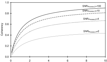
Figure 3: Coherency between linear related processes in the case of observational noise on both processes for different signal to noise ratios (SNR). The abscissa displays the SNR for one of the signals. The different curves parameterize the SNR for the other process.

Eq. (27) is of particular interest since the variance of the estimator for the phase spectrum $\widehat{\Phi}(\omega)$ depends on the coherency (Priestley 1989):

$$var(\widehat{\Phi}(\omega))=\frac{1}{\nu}\left(\frac{1}{{Coh}^{2}(\omega)}-1\right)\quad,$$ (28)

where $\nu$ is given by (25). Eq. 28 holds if the coherency is significantly larger than zero. For a coherency towards zero, the distribution of the estimated phase approaches the uniform distribution in $[-\pi,\pi]$. Therefore, the phase spectrum cannot be estimated reliably in the case of small coherency.

Using (28), theoretical phase spectra like (20) or (22) can be fitted to estimated phase spectra by a maximum likelihood procedure. We used the Levenberg–Marquardt algorithm (Press et al. 1992). This algorithm provides confidence limits for the estimated parameters, that are asymptotically valid. The asymptotic results hold in the finite case when the parameter estimates are Gaussian. In order to test whether this condition applies in our case we performed a Monte Carlo simulation for an AR[2] process under conditions analogous to those observed in the empirical data. The variance of the driving noise, i.e. the unsynchronized EMG, was set to unity, the frequency of the AR process was 10 Hz, the relaxation time 0.1 s, i.e. one period. For a sampling frequency of 300 Hz, according to (2,3) the parameters of the AR[2] process are $a_{1}=1.8922$ and $a_{2}=-0.9355$. Gaussian observational noise was added to both processes to obtain a signal to noise ratio of 10:1. Fig. 4 shows scatter plots the estimated frequency, relaxation time $\tau$ and delay $\Delta t$ for 500 realizations of the process. The Gaussianity of the estimates is clearly visible. Furthermore the estimates are uncorrelated. This is plausible since the period $T$ determines the frequency at which the phase spectrum is vastly varying, whereas the relaxation time $\tau$ is related to the steepness of the phase spectrum at the that frequency. The estimated delay time corresponds to the sampling period of $0.0033$ s due to (23). The variances and the covariance of zero are consistent with the results from the Levenberg–Marquardt algorithm. Note that the relative error in $\tau$ is much larger than that in $T$. The goodness-of-fit is judged by the $\chi^{2}$ statistic (Press et al. 1992).

Figure 4: Scatter plots of estimated frequency and relaxation time $\tau$ (a) and delay $\Delta t$ and relaxation time $\tau$ (b) from the Monte Carlo study.

The peak frequencies of the power spectra were estimated by the frequency of maximum power. A bootstrap method to obtain confidence regions for the true peak frequency will be described elsewhere (Timmer et al. 1997). Briefly, many periodograms are simulated from the estimated power spectra by the relation (11) and the power spectrum is re-estimated. The quantiles of distribution of the peak frequencies from the re-estimated power spectra yield a confidence region for the estimated peak frequency.

If two linear processes with autocorrelation functions $\mbox{ACF}_{1}(t)$ and $\mbox{ACF}_{2}(t)$ are independent, the estimated cross-correlation function $\widehat{\mbox{CCF}}(\tau)$ is Gaussian distributed as :

$$\widehat{\mbox{CCF}}(\tau)\sim{\cal N}\left(0,N^{-1}\sum_{t}\mbox{ACF}_{1}(t)\,\mbox{ACF}_{2}(t)\right)\quad.$$ (29)

Therefore, independence is difficult to infer from the cross-correlation function since the confidence interval depends on the autocorrelation functions of both processes that are in general not known. Only if one of the processes is white noise, the $95\%$ confidence interval for a zero cross-correlation function is given by $\pm 1.96N^{-1}$. Furthermore, the estimated cross-correlation function is not uncorrelated for different lags. The covariance is given by :

$$\left(\widehat{\mbox{CCF}}(\tau_{1})\widehat{\mbox{CCF}}(\tau_{2})\right)=\frac{1}{N}\sum_{t}\mbox{ACF}_{1}(t)\mbox{ACF}_{2}(t+\tau_{2}-\tau_{1}).$$ (30)

Again, the autocorrelation functions of both processes enter the equation (Brockwell and Davis 1987). If, for example, one process is white noise and the other is oscillating the cross-correlation function will show an oscillating behavior, even if the processes are independent. If the processes are not independent, (29,30) contain also the true cross-correlation function (Bartlett 1978), rendering the interpretation even more difficult.

In the following section we apply the methods introduced above to measured data of physiological tremor without synchronization in the EMG. Whether and how cross-spectral analysis can contribute to decide about the origin of synchronized EMG in the case of (enhanced) physiological tremor is discussed in a companion paper (Timmer et al. 1998). In both cases the flexor EMG appeared to have a negligible contribution to the ACC data, i.e. the coherency spectrum is most often consistent with the hypothesis that the processes are uncorrelated. Whenever there was a significant coherency it was invoked by cross talk from the extensor EMG. The amount of cross talk can be estimated from the discontinuity at lag zero of the cross-correlation function because of its instantaneous effect. The dominant contribution of the extensor is plausible since it is the anti gravity muscle. Thus, only the extensor EMG is considered in the analysis.

4 Results

It was frequently observed that a tremor appears even without synchronization in the EMG. This was interpreted as a resonance phenomenon and described by an AR process (Stiles and Randall 1967, Randall 1973, Gantert et al. 1992). Fig. 5 shows the results of the spectral and cross-spectral analysis for the data displayed in Fig. 1. Fig. 5a shows the corresponding spectra, Fig. 5b the coherency spectrum, Fig. 5c the phase spectrum and Fig. 5d the cross-correlation function estimated as described in Section 3. The straight line in Fig. 5b represents the 5% significance level for the hypothesis of zero coherency. The dashed line in Fig. 5d gives the 5% significance level for the hypothesis of zero cross-correlation assuming that at least one of the processes is white noise according to (29). The phase spectrum is shown $2\pi$ periodically for a range of $\pm 3\pi$. The confidence regions of $2\sigma$ are only given for the central curve.

Figure 5: Results for a physiological tremor without EMG synchronization. (a): power spectra (EMG: dashed line, ACC: solid line), (b): coherency spectrum, the straight line represents the 5% significance level for the hypothesis of zero coherency, (c): phase spectrum with 95% confidence intervals, (d): cross-correlation function, the dashed lines display the 5 % significance level for zero cross-correlation assuming that at least one of the processes in consistent with white noise. Confidence intervals for the power spectra and the coherency are not displayed for reasons of clarity.

The coherency spectrum seems to exhibits two peaks at approximately 8 and 12 Hz. Taking the confidence regions for the true coherency into account which are not shown for sake of clarity reveals that these peaks are not significant, but represent a single peak in the region 7 to 14 Hz. The fact that the coherency spectrum shows its maximum values in the region of the peak of the ACC power spectrum, can be explained by (27) since EMG and ACC data are contaminated with noise. Compared to Fig. 2 the phase spectrum of the data is shifted by $\pi$. Since we measured the acceleration instead of the position this results from applying (21) twice to the ACC data. For frequencies below 3 Hz the small coherency and, therefore, the large errors of the estimated phase disable its interpretation. Note that the cross-correlation function shows a periodic structure also for negative time lags. Although they are statistically not significant, one could speculate whether they give evidence for some kind of reflex feedback.

In the frame of linear stochastic processes (without reflex feedback) the different spectra and the cross-correlation function should be determined by the following six parameters.

• The characteristic times $T$ and $\tau$, determining the parameters $a_{1}$ and $a_{2}$ of the AR process modeling the mechanic properties of the musculosceletal system.

• A possible time delay $\Delta t$ between the EMG an ACC data.

• The variance $var_{EMG}$ of the white noise $\epsilon(t)$ modeling the asynchronous EMG activity.

• The variances $var_{obs.\,ACC}$ and $var_{obs.\,EMG}$ of the observational noises $\eta_{i}(t)$.

Denoting the EMG by $y(t)$, the movement of the hand by $x(t)$ and the measured values by the subscript $m$ the model reads :

$$y(t) = \epsilon(t),\qquad\epsilon(t)\sim{\cal N}(0,var_{EMG})$$ (31)

$$x(t) = a_{1}\,x(t-1)+a_{2}\,x(t-2)+y(t-\Delta t)$$ (32)

$$y_{m}(t) = y(t)+\eta_{1}(t)$$

$$\qquad\qquad\eta_{1}(t)\sim{\cal N}(0,var_{obs.\,EMG})$$

$$x_{m}(t) = x(t)+\eta_{2}(t)$$

$$\qquad\qquad\eta_{2}(t)\sim{\cal N}(0,var_{obs.\,ACC})$$

By (2,3,4,5,13,20,22,27) we fitted the parameter to the data. First, we fitted the phase spectrum without taking a possible time delay into account. This resulted in an inappropriate fit. Only the inclusion of a time delay according to (23) into the model gave a fit consistent with the data. Note, that this time delay of one sample unit does not reflect a time delay between the processes under investigation. It results from using a time-discrete model to describe an originally time-continuous process as discussed in Section 3.3. A realization of the fitted model and the estimated spectra are displayed in Fig. 6. Taking into account the errors of all estimated quantities, it shows good quantitative agreement with the empirical results of Fig. 5. The decreasing coherency for the high frequencies due to the frequency dependent signal to noise ratio and the resulting errors in the phase spectrum are well reproduced. For the low frequencies the coherency of the model seems be larger than that of the data. This phenomenon was confirmed in many data sets. The discrepancy between the data simulated by the model and the measured data results from the contribution of the heart beat to physiological tremor (Elble and Koller 1977). This additional influence on the ACC apart from the EMG is not captured by the model. Thus, the coherency of the measured data is reduced more than expected from the model that only considers the effect of observational noise.

Figure 6: Results for a linear model fitted to the data of Fig. 5.

From a comparison of Fig. 5d and 6d it can be concluded that the small oscillations of the cross-correlation for negative lags give no evidence for a reflex feedback. These oscillations appear because the cross-correlation estimates are not uncorrelated as discussed in Section 3.3.

Assuming the validity of the AR[2] model to describe the physiological tremor, one can compare the peak frequency estimated from the power spectrum (14) with that estimated from the phase spectrum according to (2,3,22). Taking the errors of the estimates into account both values are consistent.

We received similar results in 70% of the investigated series. In the other 30% of the cases an interpretation of the phase spectrum was not possible because of the poor coherency and, therefore, large errors in the phase spectrum. As discussed in Section 3 this might be simply the result of a smaller signal-to-noise ratio in the EMG and/or ACC in these cases due to a very low tremor amplitude. An estimation of the power in the ACC and EMG spectra supported this hypothesis.

5 Summary

We investigated the relation between muscle activity and physiological tremor in the case of unsynchronized EMG activity by cross-spectral analysis with special respect to the phase spectrum and the effects of observational noise. Such an analysis is not a straightforward task since one can not a priori expect a one to one relationship between one muscle and a specific mechanical measure like force, movement or acceleration due to the redundancy of the muscle system. Furthermore, the analysis is handicapped by the small tremor amplitude.

We found that this type of physiological tremor can be regarded as an AR process driven by the uncorrelated EMG activity without involving any reflex mechanisms. We showed that the phase spectrum between EMG and ACC can not be interpreted at a single frequency in terms of a delay. The phase spectrum depends on the mechanical properties of the hand, i.e. the driven part of the system, but not on the characteristics of the driving force. The behavior of the coherency spectrum can be explained as an effect of the frequency dependent signal-to-noise ratio. In addition, for low frequencies, the effect of the heart beat on the tremor further reduces the coherency between the EMG and the ACC.

Autoregressive processes of order 2 are derived from stochastic differential equations where the noise represents a force in a Newtonian sense, i.e. causing an acceleration. The conformity of the theoretical phase spectrum assuming such a process with the empirical data shows that in the case of this small amplitude hand tremor the measured EMG represents a Newtonian force by which the muscle acts on the hand.

References

• Bloomfield P (1976) Fourier analysis of time series: An introduction. John Wiley. New York

• Bartlett MS (1978) Stochastic Processes. Cambridge University Press, Cambridge

• Brockwell PJ, Davis RA (1987) Time Series: Theory and Methods. Springer, Berlin

• Deuschl G, Blumberg H, Lücking CH (1991) Tremor in reflex sympathetic dystrophy. Arch Neurol 48:1247-1252

• Elble RJ, Koller WC (1977) Mechanistic components of normal hand tremor. Electroencephal clin Neurophysiol 44:72-82

• Elble RJ, Koller WC (1990) Tremor. The Johns Hopkins University Press, Baltimore

• Elble RJ, Randall JE (1976) Motor-unit activity responsible for 8- to 12-Hz component of human physiological finger tremor. J Neurophys 39:370-383

• Fox JR, Randall JE (1970) Relationship between forearm tremor and the biceps electromyogram. J Appl Neurophys 29:103-108

• Gantert C, Honerkamp J, Timmer J (1992) Analyzing the dynamics of hand tremor time series. Biol Cybern 66:479-484

• Hannan EJ, Thomson PJ (1971) The estimation of coherency and group delay. Biometrika 58:469-481

• Honerkamp J (1993) Stochastic dynamical systems. VCH, New York

• Iaizzo PA, Pozos RS (1992) Analysis of multiple EMG and acceleration signals of various record length as a means to study pathological and physiological oscillations. Electromyogr clin Neurophysiol 32:359-367

• Journee HL (1983) Demodulation of amplitude modulated noise: A mathematical evaluation of a demodulator for pathological tremor EMG’s. IEEE Trans Biomed Eng 30:304-308

• König M, Timmer J (1997) Analyzing X-ray variability by linear state space models, Astronomy Astophys SS 124, 589-596

• Lenz FA, Zasker RR, Kwan HC, Schnider S, Kwong R, Murayama Y, Dostrovsky JO, Murphy JT (1988) Single unit analysis of the human ventral thalamic nuclear group: correlation of thalamic ”tremor cells” with the 3-6 Hz component of parkinsonian tremor. J Neuroscience 8:754-764

• Miao T. and Sakamoto K. (1995) Effects of weight load on physiological tremor: The AR representation. Applied Human Science 14:7-13

• Pashda SM, Stein RB (1973) The bases of tremor during a maintained posture. In: Control of Posture and Locomotion, Ed.: RB Stein, KG Pearson, RS Smith, JB Redford. New York. Plenum. pp 415-419

• Press HP, Teukolsky SA, Vetterling WT, Flannery BP. 1992. Numerical Recipes, Cambridge University Press, Cambridge

• Priestley MB (1989) Spectral Analysis and Time Series. Academic Press

• Randall JE (1973) A Stochastic Time Series Model for Hand Tremor. J Appl Physiol 34:390-395

• Rietz RR, Stiles RN (1974) A viscoelastic mass mechanism as a basis for normal postural tremor. J Appl Physiol 37:852-860

• Stiles NS, Randall JE (1967) Mechanical factors in human tremor frequency. J Appl Physiol 23:324-330

• Stiles NS (1980) Mechanical and Neural feedback factors in postural hand tremor of normal subjects. J Neurophys 44:40-59

• Stiles NS (1983) Lightly damped hand oscillations: Acceleration-related feedback and system damping. J Neurophys 50:327-343

• Timmer J, Gantert C, Deuschl G, Honerkamp J (1993) Characteristics of hand tremor time series. Biol Cybern 70:75-80

• Timmer J, Lauk M, Deuschl G (1996) Quantitative analysis of tremor time series. Electroencephal clin Neurophys 101:461-468

• Timmer J, Lauk M, Pfleger W, Deuschl G (1998) Cross-spectral analysis of physiological tremor and muscle activity. II. Application to synchronized EMG, submitted to Biol Cybern

• Timmer J, Lauk M, Lücking CH (1997) Confidence regions for spectral peak frequencies. Biometr J 39:849-861