Modeling noisy time series:
Physiological tremor

Abstract

Empirical time series often contain observational noise. We investigate the effect of this noise on the estimated parameters of models fitted to the data. For data of physiological tremor, i.e. a small amplitude oscillation of the outstretched hand of healthy subjects, we compare the results for a linear model that explicitly includes additional observational noise to one that ignores this noise. We discuss problems and possible solutions for nonlinear deterministic as well as nonlinear stochastic processes. Especially we discuss the state space model applicable for modeling noisy stochastic systems and Bock’s algorithm capable for modeling noisy deterministic systems.

I Introduction

One of the aims in time series analysis of complex systems is to find a dynamical model for the data [19]. A well fitting model might yield insight into the underlying process. But also if prediction is the main goal, e.g. in order to discriminate chaos from stochasticity [60, 17], or if fitted models are used to determine dynamical invariants of the system [37, 2], an optimal estimation of the parameters is desirable. Our own interest was stimulated by modeling physiological time series in order to gain insight into the underlying systems.

The dynamical models can be (time-continuous) differential or (time-discrete) difference equations. Methods to estimate parameters in differential equations can be subdivided according to whether they require an estimation of the derivatives from the data [18, 30] or not [7, 23]. Difference equation allow to use a great variety of different approaches to model the mapping from past values to the present one. These range from parametric ones [29, 2] via neural nets [44, 70, 49], radial basis functions [16, 47] and nonparametric models [68] to local linear models [17].

For all these methods a significant amount of observational noise can be a severe problem. Especially for difference equations the functional relation between past and present values will be underestimated if observational noise is not included in the model. In the first part of this paper we exemplify this for data of physiological human hand tremor. These data contain up to 50 % observational noise. Inspired by the physics of the process, linear stochastic autoregressive (AR) processes have already been suggested in 1973 to model these data [50]. In [27] these data were analyzed by a linear state space model which takes the observational noise into account. For one data set we compare these two approaches in detail. In the second part of this paper we discuss problems introduced by observational noise and possible solutions for non-linear deterministic as well as non-linear stochastic processes.

II Modeling Physiological Tremor

The outstretched hand of a healthy subject exhibits a small amplitude oscillation called physiologic tremor [22]. The movement of the hand can be measured by piezoresistive accelerometers attached at the hand. Simultaneously the flexor and extensor muscle activity is recorded. The spectra of the muscle activity data are often flat in physiological tremor reflecting an uncorrelated activity of motoneurons [64]. For an analysis of physiological tremor data in which the muscle activity is correlated and included in the modeling, see [65].

Fig. 1 displays a 2 s section of the whole 35 s measurement which is sampled with 300 Hz. The time series consist of 10240 data points covering approximately 250 periods of the oscillation. The data are normalized to zero mean and unit variance. Fig. 2 displays the periodogram, i.e. the absolute value of the Fourier transform squared. For the treatment of special problems of estimating the spectrum from the periodogram for tremor time series, see [63]. The periodogram shows on the one hand the high amount of observational noise in these data. Roughly estimating the variance of the signal by summing up the periodogram in the range from 2.5 to 12.5 Hz, and that of the noise from the remaining frequencies results in a signal-to-noise ratio of 0.93 in relative amplitudes. On the other hand the periodogram shows one broad peak around a frequency of 7.5 Hz. This peak is usually explained as a resonance phenomenon [58]. The outstretched hand is a damped oscillator which is excited by the uncorrelated muscle activity. Usually no higher harmonics show up in the periodogram indicating that the process is linear.

FIG. 1.: A 2 s section of human physiological hand tremor data.

FIG. 2.: Periodogram of the physiological tremor data set.

The autoregressive (AR) processes invented by Yule [72] are expected to fit such data well. An AR process of order $p$ is given by :

$$x(t)=\sum_{i=1}^{p}a_{i}\,x(t-i)\,+\,\epsilon(t)\quad,$$ (1)

where $\epsilon(t)$ denotes a uncorrelated Gaussian distributed random variable with mean zero and variance $\sigma^{2}$. Such a process can be interpreted, depending on the chosen parameters, as a combination of relaxators and damped oscillators [34]. For example, an AR process of order 2 that corresponds to a damped oscillator with characteristic period $T$ and relaxation time $\tau$ given by:

$$a_{1} = 2\cos\left(\frac{2\pi}{T}\right)\,\exp\,(-1/\tau)$$ (2)

$$a_{2} = -\exp\,(-2/\tau)\qquad.$$ (3)

The spectrum is given by :

$$S(\omega)=\frac{\sigma^{2}}{|1-a_{1}e^{-i\omega}-a_{2}e^{-2i\omega}|^{2}}\qquad.$$ (4)

AR processes can be generalized to the autoregressive moving average (ARMA[p,q]) processes by including past q driving noise terms in the dynamics. For theoretical reasons ARMA[p,p-1] should be preferred to AR[p] processes for modeling of sampled continuous-time processes [46]. Experience shows that differences in the results are small.

A more substantial generalization is the linear state space model (LSSM) [34] which enables the explicit modeling of observational noise $\eta(t)$ that contributes to the measured $y(t)$ :

$$\vec{x}(t) = {\bf{A}}\,\vec{x}(t-1)+\vec{\epsilon}(t),\qquad\vec{\epsilon}(t)\in{\cal{N}}(0,{\bf{Q}})$$ (5)

$$y(t) = {\bf{C}}\,\vec{x}(t)+\eta(t),\qquad\eta(t)\in{\cal{N}}(0,R)\qquad.$$ (6)

Eq. (5) describes the linear dynamics. Eq. (6) maps the dynamics to the observation including the observational noise $\eta(t)$. Another advantage of the LSSM is its capability to model superpositions of linear processes. This is not possible for AR or ARMA processes. The spectrum of a LSSM is given by :

$$S(\omega)={\bf{C}}({\bf{1}}-{\bf{A}}e^{-{\rm i}\omega})^{-1}{\bf{Q}}\left(({\bf{1}}-{\bf{A}}e^{{\rm i}\omega})^{-1}\right)^{\rm T}{\bf{C}}^{\rm T}+R\qquad.$$ (7)

The superscript $T$ denotes transposition. Spectra of AR or ARMA processes are special cases of Eq. (7).

While parameter estimation in AR models e.g. by the Burg or Durbin-Levinson algorithm is well established, parameter estimation in the LSSM is more cumbersome, see [34] for a detailed description. Usually the Expectation – Maximization (EM) algorithm is applied [21, 54]. The EM - algorithm is a general iterative procedure to estimate parameters for models in which not all variables are observable, here $\vec{x}(t)$. Denoting the joint density of $\vec{x}(t)$ and $y(t)$ given the parameters $\Theta$ by $p(x,y|\Theta)$ and the density of $\vec{x}(t)$ given the data $y(t)$ and the parameters $\Theta$ by $p(x|y,\Theta)$ the quantity :

$$L(\Theta,\Theta^{i})=<\mbox{ln}(p(x,y|\Theta))>_{p(x|y,\Theta^{i})}$$ (8)

is calculated in the $i$th Expectation step. In the Maximization step, $L(\Theta,\Theta^{i})$ is maximized with respect to $\Theta$ yielding $\Theta^{i+1}$.

In the case of the LSSM, this means that starting from some initial values for the parameters ${\bf A},{\bf Q},{\bf C},R$ the hidden dynamic variable $\vec{x}(t)$ is estimated by the Kalman filter [39] in the expectation step. Denoting the estimator of a quantity $z(t)$ based on the data $y(1),...,y(t^{\prime})$ by $z_{t|t^{\prime}}$, the covariance matrix of the estimated $\vec{x}(t)$ by $\Omega_{t|t^{\prime}}$ and the variance of the prediction errors $(y(t)-y_{t|t^{\prime}})$ by $\Delta_{t|t^{\prime}}$ the Kalman Filter reads:

$$\Omega_{t|t-1} = {\bf A}\Omega_{t-1|t-1}{\bf A}^{T}+{\bf Q}$$ (9)

$$\Delta_{t|t-1} = {\bf C}\Omega_{t|t-1}{\bf C}^{T}+R$$ (10)

$$K = \Omega_{t|t-1}{\bf C}^{T}\Delta_{t|t-1}^{-1}$$ (11)

$$\Omega_{t|t} = (1-K{\bf C})\Omega_{t|t-1}$$ (12)

$$\vec{x}_{t|t-1} = {\bf A}\vec{x}_{t-1|t-1}$$ (13)

$$y_{t|t-1} = {\bf C}\vec{x}_{t|t-1}$$ (14)

$$\vec{x}_{t|t} = \vec{x}_{t|t-1}+K(y(t)-y_{t|t-1})$$ (15)

Since the model is gaussian and linear, the density $p(x|y,\Theta)$ is completely specified by $\vec{x}_{t|t}$ and their covariances $\Omega_{t|t}$. Note, that the covariances $\Omega_{t|t}$ only depend on the model parameters, not on the data. An improvement of the estimated quantities by the so-called smoothing filter and the lengthly equations for the parameter update of ${\bf A},{\bf Q},{\bf C},R$ in the Maximization step are given in [34]. This procedure is iterated until some convergence criterion is fulfilled.

There are different criteria to judge the goodness of fit of a dynamical model.

• Whiteness of the prediction errors. The model should explain all correlations in the data yielding uncorrelated prediction errors. By the Kolmogorov - Smirnov test [48] it can be tested whether the periodogram of the prediction residuals is consistent with white noise [12].

• A knee in the variance of the prediction errors for ascending model order indicates the correct order. Criteria like AIC [3], BIC [53], MDL [52] can be used to take into account the different number of parameters in the compared models. The application of these criteria is not without problems [1]. If the model class is not correct, these criteria will choose ”some” order.

• The distribution of some feature can be derived from numerous realizations of the model and the compatibility of the value of the feature calculated from the data with this distribution can be examined, see e.g. [71].

In the case of linear modeling there are two more criteria.

• Since the parameters in linear models are related to relaxation times of the corresponding oscillators and relaxators, negligible relaxation times indicate a to large model order.

• According to Eq. (7) the spectra of linear processes can be calculated from the parameters of the estimated models. Since the spectrum is the expectation of the periodogram, a comparison of the spectrum to the periodogram of the data serves as a qualitative criterion.

We now present the results of the analysis of the data shown in Fig. 1. We do not give the estimated parameter here since they are rather uninformative. Instead, Tab. 1 displays the resulting periods and relaxation times. These characteristic times can be calculated for any model order by formulas analogous to Eqs. (2,3) [34].

model order	AR model			LSS model
	relaxation	period	prob.	relaxation	period	prob.
	time		WN	time		WN
1	1.2	-	0	7.9	-	0
2	2.9	-	0	91.9	39.9	0.24
	1.0	-		-	-
3	4.8	-	10-8	91.9	39.9	0.27
	1.3	6.5		0.2	-
4	6.6	-	10-7	91.9	39.9	0.23
	1.6	4.3		9.0	8.3
	1.4	-		-	-
5	7.5	-	10-8	91.9	39.9	0.24
	1.5	4.3		9.4	8.4
	1.2	11.9		0.6	-

TAB. 1. Relaxation times and periods of the fitted AR and LSS models of ascending order for the physiological tremor data. ”prob. WN” denotes the probability of the residuals to be consistent with white noise.

For an estimated oscillator a relaxation time smaller than the period of the oscillation indicates that this oscillator is insignificant. Pure relaxators with an relaxation time of a few time steps have also to be regarded as negligible. For the LSSM, a model order of two with a period of approximately 40 time steps, corresponding to a frequency of 7.5 Hz, and a relaxation time of 91 time steps is clearly identified. For the AR models no significant structure is detected. Tab. 1 also gives the probability of the residuals to be consistent with white noise. For the LSSM, models with an order larger than one yield prediction residuals which are consistent with white noise. The residuals of the AR processes are not consistent with white noise for all model orders investigated.

Fig. 3 displays the variance of the prediction error in dependence on the model order. The graph for the LSSM exhibits a clear cut knee at an order of 2 whereas the graph of the AR model does not allow for a clear cut decision. The graph saturates around order 5 and decreases slowly for larger orders. We fitted AR model up to order 50 and applied the AIC. Even for this unrealistic high orders the function AIC(p) still decreases.

Fig. 4 shows a quantile-quantile – plot with respect to a Gaussian distribution of the normalized prediction residuals for the LSSM of order two and the expected straight line. Only ten of the 10240 points deviate from the straight line indicating Gaussianty of the prediction residuals.

All these results indicate that the LSSM of order two describes the data adequately. Fig. 5 displays the low frequency part of spectrum estimated from the parameters of the fitted LSSM of order two and the periodogram of the data. This confirms the above results.

FIG. 3.: Residual variance of the fitted AR (+) and LSS ($\Diamond$) models in dependence on the model order.

FIG. 4.: Quantile-quantile plot of the normalized prediction residuals of the second order LSSM with respect to a Gaussian distribution. The straight gives the expected behavior in the case of Gaussianity.

In terms of physics and physiology these result show that the physiological tremor is a linear damped oscillation driven by uncorrelated muscle activity. The parameters of the model describe the mechanical properties of the muscle-hand system, i.e. its mass, stiffness and damping.

III Modeling Noisy Time Series

The behavior of the AR model in the previous section, i.e. not recovering the correct model order, is caused by the observational noise. Whereas the LSSM includes the observational noise explicitly in the model, the AR model assumes the data to be free from observational noise. We use a simple first order process to demonstrate the consequences. In an AR[1] model

$$x(t)=ax(t-1)+\epsilon(t)$$ (16)

the parameter $a$ can be estimated without bias by :

$$\hat{a}=\frac{\sum x(t-1)x(t)}{\sum x(t-1)x(t-1)}\quad.$$ (17)

FIG. 5.: Periodogram of the data (dotted) and spectrum of the fitted second order linear state space model (solid).

If the dynamics is covered by observational noise:

$$y(t)=x(t)+\eta(t),\qquad\eta(t)\sim{\cal{N}}(0,R)\quad,$$ (18)

the expected value of $\hat{a}$ estimated analogously to Eq. (17) from $y(t)$ is

$$<\hat{a}>=\frac{<y(t-1)y(t)>}{<y(t-1)y(t-1)>}=a\,\frac{1}{1+\frac{R}{<x(t)^{2}>}}\quad.$$ (19)

Thus, the parameter $a$ is underestimated. The degree of the underestimation depends on the signal-to-noise ratio. This effect is known from linear regression theory where it is called the ”Error-in-variables” - problem [26] and was first mentioned in the context of time series in [42]. For the data analyzed in the previous section the variance of the signal nearly equals the variance of the noise. Thus, an underestimation of $a$ by a factor of two is expected. Indeed, even for the misspecified first order models, the parameter estimated from the LSSM is $0.882$ and that for the AR[1] model is $0.443$. Note, that in the case of second order models the misestimation of the parameters for the AR[2] models leads to a detection of two relaxators, whereas the LSSM recognizes the oscillator, see Tab. 1. Thus the AR model leads to a wrong interpretation.

The underestimation of the functional relation between past and present values in the case that observational noise is not taken into account carries over to more general models. Assuming stationarity of the underlying process systems can be linear or nonlinear, resp. deterministic or stochastic. Our approach to discriminate deterministic from stochastic systems, i.e. the presence of dynamical noise, is rather practical. For example, in the data analyzed in the previous section it is imaginable to model the muscle activity by a deterministic system, including a model for the brain and the spinal tract. This would result in a very high dimensional dynamical system whose output is equally well captured by white noise. Thus, whenever a huge amount of influences enters the system significantly a stochastic description might be recommended. But also if there exists no shadowing trajectory for a realization of deterministic system, the use of stochastic models might be indicated [20].

The dynamics can be described by differential equation or by maps. In the following we discuss possible treatments of observational noise in the different cases. If present the dynamical noise is assumed to be Gaussian and additive. By the latter assumption we exclude models which are able to describe fluctuations in the parameters, e.g. bilinear models [59].

A Linear deterministic case

The linear deterministic case is easy to treat since the solutions of the dynamical equations are explicitly known and can be fitted to the noisy data. Parameters of continuous- and discrete-time modeling are connected by equations like Eq. (2,3). An application to physiological data is given in [32].

B Linear stochastic case

The linear stochastic case is solved by the state space model discussed above. Because of the linearity and gaussianity of the model there is a direct connection between the parameters from discrete-time and those from the continuous-time models. Parameter estimation for the continuous-time case is presented in [57]. An application of the state space model to astrophysical data is given in [41].

C Nonlinear deterministic case

The effect of observational noise is different for fitting differential and difference equations to the data.

For modeling data by differential equations two approaches can be distinguished depending on whether time derivatives of the process has be estimated from the data or not. Since estimating derivatives form the data amplifies the noise, the former method as applied in [18, 11, 24, 30, 31, 35] is vulnerable to significant amounts of observational noise as demonstrated in [35].

To fit differential equations to noisy deterministic data without estimating derivatives from the data, at least two different approaches exist. In the initial value approach one chooses some initial parameters in the model and an initial value for the trajectory, integrates the differential equation and tries to minimize the prediction error by some minimization algorithm [23]. Without many precautions, this procedure has been shown to be unstable, i.e. yielding divergent trajectories, and is susceptible to stopping in a local minimum [51, 66]. A more sophisticated algorithm was developed by Bock [6, 7]. His elegant multiple shooting approach starts with a discontinuous trajectory which stays close to the data. The continuity of the underlying trajectory enters into the algorithm by a constraint in the cost function. This constraint is nonlinear in the parameters but enters the optimizing strategy only in a linearized way. Therefore, the trajectory is allowed to be discontinuous at the beginning of the iteration but is forced to become continuous in the end.

We illustrate the behavior of Bock’s algorithm by the restricted Lotka-Volterra system which has been used to compare different fitting procedures [8, 69, 67, 23]:

$$\dot{x}_{1} = k_{1}x_{1}-k_{2}x_{1}x_{2}$$ (20)

$$\dot{x}_{2} = k_{2}x_{1}x_{2}-k_{3}x_{2}$$ (21)

with the parameters $k_{1}=1.0$, $k_{2}=1.5$ and $k_{3}=2.0$ and initial values $x_{1}(0)=0.3$, $x_{2}(0)=0.8$. The system is integrated by the routine BSSTEP from [48] for 20 s and sampled with $\Delta t=0.2$ s. The standard deviation of the data is 1.09. Observational noise with standard deviation of 0.5 was added to the signal. To fit the parameters, only the first component was used. All starting points for the second component were set to 0.5. Initial values for the parameter estimates were $\hat{k}_{1}=0.5$, $\hat{k}_{2}=0.75$ and $\hat{k}_{3}=1.0$. 30 starting points were used for the initially discontinuous trial trajectory. Fig. 6 shows initial situation (A), the third iteration (B) and the converged solution (C) after 16 iterations of the algorithm. The true trajectory is reproduced well. With respect to the confidence regions, the estimated parameters are compatible with the true parameters: $\hat{k}_{1}=1.01\pm 0.14$, $\hat{k}_{2}=1.53\pm 0.34$ and $\hat{k}_{3}=2.02\pm 0.45$.

Simulation studies comparing both algorithms show that Bock’s algorithm is more stable and converges to the global minimum for a larger set of initial guesses for the parameters than the initial value approach [51, 66]. Note, that for both approaches it is not necessary to reconstruct the dynamics by delay-embedding [61] avoiding all problems related to choosing the delay time [43].

In a simulation study Bock’s algorithm has been successfully applied to model noisy chaotic data from dissipative as well as conservative systems [4, 38]. Applications of this method to chemical and physiological data are reported in [6, 5]. The basic idea of Bock’s algorithm, i.e. taking advantage of the fact that the process under investigation has produced a continuous trajectory, carries over to modeling noisy deterministic systems by maps. Nevertheless this idea has not attracted much attention and modeling data by maps is generally treated as a regression not as a dynamical problem.

Stimulated by [19] a large number of different approaches have been suggested to model nonlinear dynamics by maps. They are distinguished by the type of basis function used to approximate the nonlinear functional relationship between past values and the present one. Amongst others, polynomials [29], sigmoidals [44, 70, 49], radial basis functions [47] and local linear models [17] have been suggested. Analogous to the AR model discussed above all these methods are subject to the ”Error-in-variables” – problem. For the tremor data and the AR model of order two in Sec. II above this problem led to a detection of two relaxators instead of an oscillator. In [37] it was reported that observational noise covering chaotic data led to a detection of a periodic process. That might be caused by the same phenomenon of underestimated parameters.

The generalization of the theory of ”Error-in-variables” from nonlinear regression, see [15] for a recent review, to modeling of noisy nonlinear deterministic time series by maps and an application to empirical data are presented in [36].

FIG. 6.: Convergence of Bock’s algorithm for the noisy Lotka-Volterra system. A: Initial situation. B: After the third iteration. C: After convergence, dashed line: true trajectory.

D Nonlinear stochastic case

For the nonlinear stochastic case, including a possible nonlinear mapping $g(.)$ of the state vector $\vec{x}(t)$ to the observation $y(t)$ :

$$\dot{\vec{x}}(t) = \vec{f}(\vec{x}(t))+\vec{\epsilon}(t),\qquad\vec{\epsilon}(t)\in{\cal{N}}(0,{\bf{Q}})$$ (22)

$$y(t) = g({\vec{x}}(t))\,+\eta(t),\qquad\eta(t)\in{\cal{N}}(0,R)\qquad,$$ (23)

a generalization of the Kalman filter Eq. (9-15) appears to be the solution. Therefore, for the discrete-time version, the matrices $\bf{A}$ and $\bf{C}$ are replaced by linear approximations of $\vec{f}(\vec{x}(t))$ and $g({\vec{x}}(t))$ [28, 45]:

$$\bf{A} = \frac{\partial\vec{f}}{\partial\vec{x}}\left|{}_{\vec{x}=\vec{x}_{t-1|t-1}}\right.$$ (24)

$$\bf{C} = \frac{\partial g}{\partial\vec{x}}\left|{}_{\vec{x}=\vec{x}_{t|t-1}}\right.$$ (25)

This solution is, in general, not valid for two reasons. First, as mentioned in Sec. II, the variance $\Omega_{t|t}$ of the predicted state variable $\vec{x}_{t|t}$ depends only on the model, i.e. not on the amount of data, and might be so large that the linearization is not valid. Thus, the distribution of $\vec{x}_{t|t}$ becomes nongaussian and a first and second order description is not sufficient. Second, the noise will become nongaussian in time-discrete nonlinear models. This results from the theory of integrating stochastic differential equations, see [40] for a recent review. One main result of this theory is that unlike deterministic differential equations, stochastic ones can not be integrated by arbitrary high order methods, e.g. by integrating the deterministic part by a Runge-Kutta method of 4.th order and adding some noise to the resulting value. Due to complicated stochastic integrals in the Taylor expansion for higher order integration schemes, only first or second order methods are feasible. Therefore, usually, the process has to be integrated on a much smaller time scale than it is observed. This turns the effective noise on the time scale of the observation nongaussian. Because of this effect methods like those proposed in [9, 10] are applicable in special cases only.

The nongaussianity prevents a maximum likelihood estimation of the parameter. A least square approach yields biased estimates [33]. In general, for nongaussian distributions all higher moments have to be taken into account. A truncated expansion in moments was suggested in [28], the application of the Gibbs sampler using a mixture of normals to approximate the distributions was introduced in [14]. To our knowledge no application of these methods to empirical data have been reported.

All the map-based methods mentioned in Sec. III C can be applied to nonlinear stochastic system by allowing for a residual error in the prediction. Here, the above mentioned non-gaussianity is also a problem since commonly applied least square fitting is no longer maximum likelihood.

An application of the ”Error-in-variables”-theory to this double stochastic situation is not straightforward. To apply this theory, the ratio of the variance of the noise of past values to that of the present value must be known. The noise covering the past values is simply the observational noise, but the noise on the present value is, in contrast to pure regression, the sum of the observational and the dynamical noise. Since spectra of most (observational noise free) processes decay for high frequencies [56, 55], the variance of the observational noise can be estimated from this region. But the variance of the dynamical noise is usually obtained after fitting the model since minimizing this variance is the optimizing criterion.

The severity of the effects of the problems discussed depends on the system, i.e. the type of the nonlinearity and the variances of dynamical and observational noise. We demonstrate this by briefly reporting the results of modeling a time series of Parkinsonian tremor. This type of tremor is believed to be a nonlinear process [27, 62]. The time series was recorded under the same conditions as the physiological tremor data analyzed in Sec. II. Fortunately, the observational noise in these data is negligible small. Using a large variety of ansatzes for the right hand side of the differential equation, we did not succeed in fitting a nonlinear deterministic differential equation by Bock’s algorithm to the data. Therefore, we assumed that the process is stochastic and tried global polynomials that are orthogonal with respect to the measure given by the data. These polynomials were discussed in the context of regression theory by Forsythe [25]. He also introduced a recursive algorithm to determine the polynomials and their coefficients. In [29, 13, 2] they were made popular for the analysis of time series. As discussed in [2] the significance of each single polynomial can be judged independently from the other polynomials.

Using models of polynomial order 4 and an embedding delay $\tau$ of 10 time steps we fitted models of ascending autoregression order to the data. We found a model of regression order 3 containing 16 significant parameters which describes the data adequately. The goodness of fit was judged by a clear cut knee in the residual variance (Fig. 7),

FIG. 7.: Variance of the prediction errors for 4.th order polynomial models of ascending autoregression order.

the whiteness of the residuals (Fig. 8) and a comparison of the spectra of the empirical data and data realized from

FIG. 8.: Kolmogorov-Smirnov test statistic D for the consistency of the prediction errors with white noise of 4.th order polynomials models of ascending autoregression order. The 5 % significance level is marked.

the model (Fig. 9). Note, that in Fig. 9 also the small peak near 13.5 Hz which is only due to aliasing because of the effective downsampling by choosing $\tau=10$, is reproduced by the model.

   

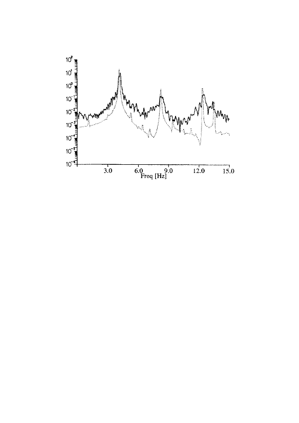
FIG. 9.: Spectrum estimated from the original data (solid line) and from a realization of the fitted model (dotted line).

Unfortunately we did not succeed in assigning a physiologic meaning to the fitted parameters.

IV Discussion

The project ”Equations of Motion from a Data Series” [19] has attracted much attention. Our own interest was to obtain models for physiological data like EEG or tremor. The hope was to learn something about the underlying systems from the fitted models. In the first part of this paper we gave an example where this idea could be fulfilled and the parameter of the fitted model could be interpreted in terms of physics and physiology. This was facilitated by the fact that the well understood theory of linear systems was applicable.

In the general case of nonlinear deterministic or even nonlinear stochastic systems it appears to be much harder to obtain such a result. This is on the one hand caused by the fact that the treatment of observational noise is not solved in general. On the other hand without much knowledge about the system under investigation, it is hard to decide on a certain interpretable ansatz for the parameterization of the nonlinear dynamics.

Often an interpretable model is not the goal of modeling, e.g. if only prediction as for stock market data or the temporal evolution of the prediction error as for discriminating deterministic from stochastic behavior is the aim. But here also observational noise is a problem, since the functional relationship will be underestimated if it is modeled by maps. A model taking this noise into account would lead to a better model and a smaller prediction error.

Results for fitted differential equations might be compared to known systems in order to understand the underlying mechanisms. For maps this seems to be much more difficult, especially when sigmoidals, radial basis functions or local linear models are used as basis functions. But even if global polynomials are used an assignment of a physical meaning to the parameters is difficult since a single parameter in the underlying differential equation shows up in the coefficients of more than one basis function. Furthermore, the model structure depends on the sampling time.

For many methods applied to model time series, observational noise causes problems since these methods treat the data as in regression. For deterministic systems Bock’s algorithm provides an elegant alternative which explores the additional information that the process under investigation produced a continuous trajectory.

There is growing evidence that many physiological processes are neither linear stochastic processes since surrogate data testing reject this hypothesis nor nonlinear deterministic processes since low dimensional attractors can not be established. Therefore, we believe that methods to model (noisy) nonlinear stochastic processes are worth being studied in more detail.

Data availability

The tremor data and the simulated data of the Lotka-Volterra system are accessible at:
http://phym1.physik.uni-freiburg.de/$\sim$jeti/tremordata/

REFERENCES

- [1] L.A. Aguirre. Some remarks on structure selection for nonlinear models. Int. J. Bif. Chaos, 4:1707–1714, 1994.
- [2] L.A. Aguirre and S.A. Billings. Retrieving dynamical invariants from chaotic data using NARMAX models. Int. J. Bif. Chaos, 5:449–474, 1995.
- [3] H. Akaike. Information theory and an extension of the maximum likelihood principle. In B.N. Petrov and F. Csaki, editors, 2nd International symposium on information theory, Budapest, 1973. Akademiai Kiado.
- [4] E. Baake, M. Baake H.G. Bock, and K.M. Briggs. Fitting ordinary differential equations to chaotic data. Phys. Rev A, 45:5524–5529, 1992.
- [5] E. Baake and J.P. Schlöder. Modeling the fast flourescence rise of photosynthesis. Bull. Math. Biol., 54:999–1021, 1992.
- [6] H.G. Bock. Numerical treatment of inverse problems in chemical reaction kinetics. In K.H. Ebert, P. Deuflhard, and W. Jäger, editors, Modelling of chemical reaction Systems, volume 18, pages 102–125, New York, 1981. Springer.
- [7] H.G. Bock. Recent advances in parameteridentification for ordinary differential equations. In P. Deuflhard and E. Hairer, editors, Progress in Scientific Computing, volume 2, pages 95–121, Boston, 1983. Birkhäuser.
- [8] H.G. Bock. Randwertproblemmethoden zur Parameteridentifizierung in Systemen nichtlinearer Differentialgleichungen. Dissertation, Universität Bonn, Bonner Mathematische Schriften 183, Bonn, 1987.
- [9] L. Borland and H. Haken. Unbiased determination of forces causing observed processes. Z. Phys. B - Cond. Matt., 88:95–103, 1992.
- [10] L. Borland and H. Haken. Unbiased estimate of forces from measured correlation functions, including the case of strong multiplicative noise. Ann. Phys., 1:452–459, 1992.
- [11] J.L. Breeden and A. Hübler. Reconstructing equations of motion from experimental data with unobserved variables. Phys. Rev. A, 42:5817–5826, 1990.
- [12] P.J. Brockwell and R.A. Davis. Time Series: Theory and Methods. Springer, New York, 1987.
- [13] R. Brown. Calculating Lyapunov exponents for short and/or noisy data sets. Phys. Rev. E, 47:3962 – 3969, 1993.
- [14] B.P. Carlin, N.G. Polson, and D.S. Stoffer. A Monte – Carlo approach to nonnormal and nonlinear state – space modelling. J. Am. Stat. Ass., 87:493 – 500, 1992.
- [15] R.J. Carroll, D. Ruppert, and L.A. Stefanski. Measurement Error in Nonlinear Models. Chapman and Hall, London, 1995.
- [16] M. Casdagli. Nonlinear prediction of chaotic time series. Physica D, 35:335 – 356, 1989.
- [17] M. Casdagli. Chaos and deterministic versus stochastic nonlinear modeling. J. Roy. Stat. Soc. B, 54:303–328, 1991.
- [18] J. Cremers and A. Hübler. Construction of differential equations from experimental data. Z. Naturforsch., 42a:797–802, 1987.
- [19] J.P. Crutchfield and B.S. McNamara. Equations of motion from data series. Complex Systems, 1:417, 1987.
- [20] S. Dawson, C. Grebogy, T. Sauer, and J.A. Yorke. Obstructions to shadowing when a Lyapunov exponent fluctuates about zero. Phys. Rev. Lett., 73:1927–1930, 1994.
- [21] A.P. Dempster, N.M. Laird, and D.B. Rubin. Maximum likelihood from incomplete data via EM algorithm. J. Roy. Stat. Soc., 39:1–38, 1977.
- [22] G. Deuschl, P. Krack, M. Lauk, and J. Timmer. Clinical neurophysiology of tremor. J. Clinic. Neurophys., 13:110–121, 1996.
- [23] L. Edsberg and P. Wedin. Numerical tools for parameter estimation in ODE-systems. Opt. Meth. Software, 6:193–217, 1995.
- [24] T. Eisenhammer, A. Hübler, N. Packard, and J.A.S. Kelso. Modeling experimental time-series with ordinary-differential equations. Biol. Cybern., 65:107–112, 1991.
- [25] G.E. Forsythe. Generation and use of orthogonal polynomials for data – fitting with a digital computer. J. Soc. Indust. Appl. Math., 5:74–88, 1957.
- [26] W.A. Fuller. Measurement error models. John Wiley, New York, 1987.
- [27] C. Gantert, J. Honerkamp, and J. Timmer. Analyzing the dynamics of tremor time series. Biol. Cybern., 66:479–484, 1992.
- [28] A. Gelb. Applied Optimal Estimation. MIT – Press, Cambrigde, 1989.
- [29] M. Giona, F. Lentini, and V. Cimiagalli. Functional reconstruction and local prediction of chaotic time series. Phys. Rev. E, 44:3496 – 3502, 1991.
- [30] G. Gouesbet. Reconstruction of the vector fields of continuous dynamical systems from scalar time series. Phys. Rev. A, 43:5321–5331, 1991.
- [31] G. Gouesbet and J. Maquet. Construction of phenomenological models from numerical scalar time series. Physica D, 58:202–215, 1992.
- [32] D.R. Groothuis, G.D. Lapin, F.J. Vriesendorp, M.A. Mikhael, and C.S. Patlak. A method to quantitatively measure transcapillary transport of iodinated compounds in cauine brain tumors with computed tomography. J. Cer. Blood Flow Metabol., 11:939–948, 1991.
- [33] A.C. Harvey. Forecasting structural time series models and the Kalman filter. Cambridge University Press, 1994.
- [34] J. Honerkamp. Stochastic Dynamical Systems. VCH, New York, 1993.
- [35] A.D. Irving and T. Dewson. Determining mixed linear-nonlinear coupled differential equations from multivariate discrete time series sequences. Physica D, 102:15–36, 1997.
- [36] L. Jaeger and H. Kantz. Unbiased reconstruction of the dynamics underlying a noisy chaotic time series. Chaos, 6:440–450, 1996.
- [37] J.B. Kadtke, J. Brush, and J. Holzfuss. Global dynamical equations and Lyapunov exponents from noisy chaotic time series. Int. J. Bif. Chaos, 3:607–616, 1993.
- [38] J. Kallrath, J.P. Schlöder, and H.G. Bock. Least squares parameter estimation in chaotic differential equations. Cel. Mech. Astro. Dyn., 56:353–371, 1993.
- [39] R.E. Kalman. A new approach to linear filtering and prediction problems. Trans. ASME J. Basic Eng. Series D, 82:35–46, 1960.
- [40] P.E. Kloeden, E. Platen, and H. Schulz. The numerical solution of nonlinear stochastic dynamical systems: a brief introduction. Int. J. Bif. Chaos, 1:277–286, 1991.
- [41] M. König and J. Timmer. Analyzing X-ray variability by linear state space models. Astronomy Astrophys. SS, 124:589–596, 1997.
- [42] E.J. Kostelich. Problems in estimating dynamics from data. Physica D, 58:138, 1992.
- [43] D. Kugiumtzis. State space reconstruction parameters in the analysis of chaotic time series - the role of the time window length. Physica D, 95:13–28, 1996.
- [44] A. Lapedes and R. Farber. Nonlinear signal processing using neural networks. Technical Report LA-UR-87-2662, Los Alamos National Laboratory, Los Alamos, NM, 1987.
- [45] J.M. Mendel. Lessons in estimation theory for signal processing, communications and control. Prentice Hall, New Jersey, 1995.
- [46] M.S. Phadke and S.M. Wu. Modeling of continuous stochastic processes from discrete observations with application to sunspots data. J. Am. Stat. Ass., 69:325–329, 1974.
- [47] T. Poggio and F. Girosi. Networks for approximation and learning. Proc. IEEE, 78:1481–1497, 1990.
- [48] W.H. Press, B.P. Flannery, S.A. Saul, and W.T. Vetterling. Numerical Recipes. Cambrigde University Press, Cambrigde, 1992.
- [49] J.C. Principe, A. Rathie, and J.M. Kuo. Prediction of chaotic time series with neural networks and the issue of dynamic modeling. Int. J. Bif. Chaos, 2:989–996, 1992.
- [50] J.E. Randall. A stochastic time series model for hand tremor. J. Appl. Phys., 34:390 – 395, 1973.
- [51] O. Richter, P. Nörtersheuser, and W. Pestemer. Non-linear parameter estimation in pesticide degradation. Science Total Env., 123/124:435–450, 1992.
- [52] J. Rissanen. Modeling by shortest data description. Automatica, 14:465–471, 1978.
- [53] G. Schwartz. Estimating the order of a model. Ann. Stat., 6:461–464, 1978.
- [54] R.H. Shumway and D.S. Stoffer. An approach to time series smoothing and forecasting using the EM algorithm. J. Time Ser. Anal., 3:253–264, 1982.
- [55] D. Sigeti. Survival of deterministic dynamics in the present of noise and the exponential decay of power spectra at high frequency. Phys. Rev. E, 52:2443–2457, 1995.
- [56] D. Sigeti and W. Horsthemke. High-frequency power spectra for systems subject to noise. Phys. Rev. A, 35:2276–2282, 1987.
- [57] H. Singer. Continous-time dynamical systems with sampled data, errors of measurement and unobserved components. J. Time Ser. Anal., 14:527–545, 1993.
- [58] R.N. Stiles. Mechanical and neural feedback factors in postural hand tremors of normal subjects. J. Neurophys., 44:40–59, 1980.
- [59] T. Subba Rao and M.M. Gabr. An introduction to bispectral analysis and bilinear time series models. Springer, New york, 1984.
- [60] G. Sugihara and R.M. May. Nonlinear forecating as a way of distinguishing chaos from measurement error in time series. Nature, 344:734–741, 1990.
- [61] F. Takens. Detecting strange attractors in turbulence. In D.A: Rand and L.S. Young, editors, Dynamical Systems and Turbulence, volume 898 of Lecture Notes in Mathematics, pages 366–381, Berlin, 1981. Springer.
- [62] J. Timmer, C. Gantert, G. Deuschl, and J. Honerkamp. Characteristics of hand tremor time series. Biol. Cybern., 70:75–80, 1993.
- [63] J. Timmer, M. Lauk, and G. Deuschl. Quantitative analysis of tremor. Electroenceph. clin. Neurophys., 101:461–468, 1996.
- [64] J. Timmer, M. Lauk, W. Pfleger, and G. Deuschl. Cross-spectral analysis of physiological tremor and muscle activity. I. Theory and application to unsynchronized EMG. Biol. Cybern. in press, 1998.
- [65] J. Timmer, M. Lauk, W. Pfleger, and G. Deuschl. Cross-spectral analysis of physiological tremor and muscle activity. II. Application to synchronized EMG. Biol. Cybern. in press, 1998.
- [66] J. Timmer, T. Müller, and W. Melzer. Numerical methods for the determination of calcium release from calcium transients in muscle cells. Biophys. J. in press, 1998.
- [67] I. Tjoa and L. Biegler. Simultaneous solution and optimization strategies for parameter estimation of differential-algebraic equation systems. Indust. Eng. Chem. Res., 30:376–385, 1991.
- [68] D. Tjostheim and B.H. Auestad. Nonparametric identification of nonlinear time series: Selecting significant lags. J. Am. Stat. Ass., 89:1410–1419, 1994.
- [69] J.M. Varah. A spline least squares method for numerical parameter estimation in differential equations. SIAM J. Scient. Stat. Comp., 3:28–46, 1982.
- [70] A.S. Weigend, B.A. Huberman, and D.E. Rumelhart. Predicting the future: A connectionist approach. Int. J. Neur. Comp., 1:193–209, 1990.
- [71] A. Witt, J. Kurths, F. Krause, and K. Fischer. On the validity of a model for the reversals of the earths magnetic-field. Geophys. Astrophys. Fluid Dynamics, 77:79–91, 1994.
- [72] G.U. Yule. On a method of investigating periodicities in disturbed series, with special reference to wolfer’s sunspot numbers. Phil. Trans. R. Soc. A, 226:267–298, 1927.