Hydrodynamics and Radiation
from a Relativistic Expanding Jet
with Applications to GRB Afterglow

Abstract

We describe fully relativistic three dimensional calculations of the slowing down and spreading of a relativistic jet by an external medium like the ISM. We calculate the synchrotron spectra and light curves using the conditions determined by the hydrodynamic calculations. Preliminary results with a moderate resolution are presented here. Higher resolution calculations are in progress.

Introduction

The level of beaming in GRBs is one of the most interesting open questions in this subject. The relativistic flow which drives a GRB may range from isotropic to strongly collimated into a narrow opening angle. The degree of collimation (beaming) of the outflow has many implications on most aspects GRB research, such as the requirements from the “inner engine”, the energy release and the event rate. During the prompt emission the Lorentz factor of the flow is very high ($\gamma>100$), and due to relativistic aberration of light, only a narrow angle of $\sim 1/\gamma$ around the line of sight (LOS) is visible. During the afterglow stage, the flow decelerates and an increasingly larger angle becomes visible. As long as $\gamma>1/\theta$ an outflow collimated within an angle $\theta$ around the LOS produces the same observed radiation as if it were part of a spherical outflow. Once $\gamma$ drops below $1/\theta$, the observer can notice that radiation arrives only from within an angle $\theta$ around the LOS, instead of $1/\gamma$ as in the spherical case. Sideways expansion is also expected to become important when $\gamma\sim 1/\theta$ Rhoads ; SPH . These two effects combine to create a break in the light curve at $\gamma\sim 1/\theta$, but it is not quite clear whether this break is sharp enough to be detected Rhoads ; SPH ; WL . To explore this question we have performed fully relativistic three dimensional simulations that follow the slowing down and the lateral expansion of a relativistic jet. We then calculate the synchrotron light curve and spectrum using the conditions determined by the hydrodynamical simulation.

The Hydrodynamics

We use a fully relativistic three dimensional code for the hydrodynamical calculations. The initial conditions are a wedge with an opening angle $\theta_{0}=0.2$ taken from the Blandford McKee BM , BM hereafter, self similar spherical solution, embedded in a cold and homogeneous ambient medium. For this initial opening angle, the jet is expected to show considerable lateral expansion when $\gamma\sim 1/\theta_{0}=5$, where $\gamma$ is the Lorentz factor of the fluid. The BM solution used for the initial conditions was therefore at the time when $\Gamma=10$, where $\Gamma=\sqrt{2}\gamma$ is the Lorentz factor of the shock. The total isotropic energy was $E=10^{52}\ {\rm ergs}$, and the ambient number density was $n=1\ {\rm cm^{-3}}$.

In Figures 2-5 we present snapshots of the number density, internal energy density, Lorentz factor and velocity field of the fluid, as the jet slows down and spreads sideways. An explanation of what is seen in these snapshots is given in Figure 1. The snapshots are taken at consecutive times, ranging $t=137-282\ {\rm days}$ in the rest frame of the ambient medium (corresponding roughly to observer times from one and a half to twenty days for an observer along the jet axis). The results shown in this work are still preliminary. The resolution is not sufficient to resolve the very thin initial shell. For this reason the maximal Lorentz factor of the matter is just over $3$, instead of $10/\sqrt{2}\cong 7.07$ (see Figure 4). Higher resolution runs are in progress.

Calculating Light Curves and Spectra

The local emission coefficient at a given space-time point is calculated directly from the hydrodynamical quantities there. The magnetic field and electron energy densities are assumed to hold constant fractions, $\epsilon_{B}$ and $\epsilon_{e}$, respectively, of the internal energy, while the electrons posses a power law energy distribution, $N(\gamma_{e})\propto\gamma_{e}^{-p}$. The local emissivity is approximated by a broken power law: $F_{\nu}\propto\nu^{1/3}$ and $\ \nu^{(1-p)/2}$, below and above the typical synchrotron frequency, respectively GPS .

The light curves and spectra are calculated for several viewing angles with respect to the jet axis. Once the emission coefficient is determined in the local frame, it is transformed to the frame of each observer. The time of arrival to each observer is then calculated, and the contributions are sumed over space-time, producing the various light curves. This is done for several frequencies, simultaneously, so that the spectrum may be obtained, as well as the light curve at different frequencies.

A few light curves, calculated for $\epsilon_{B}=\epsilon_{e}=0.1$ and $p=2.5$, are shown in Figure (6). These light curves serve to demonstrate the potential of this approach. Future simulations are expected to achieve sufficient resolution to produce realistic light curves which could be compared with afterglow observations.

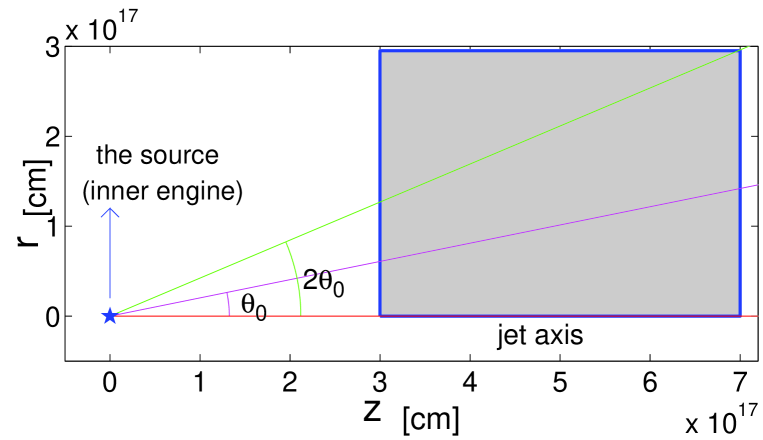
Figure 1: The region depicted in Figures (2-5) is within the shaded region, outlined in blue. $z$ and $r$ are the cylindrical coordinates. The jet axis is in the $z$ direction. Two colored lines which indicate opening angles of $\theta_{0}$ and $2\theta_{0}$ are added to help follow the lateral expansion.

Figure 2: The proper number density, in ${\rm cm^{-3}}$.

Figure 3: The internal energy density, in units of $m_{p}c^{2}/{\rm cm^{3}}$.

Figure 4: The bulk Lorentz factor of the fluid.

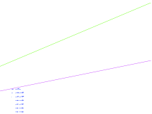
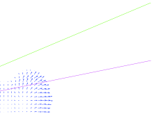
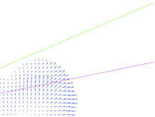
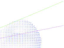
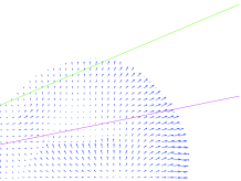
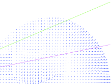
Figure 5: The velocity field of the fluid. Each arrow points at the direction of the velocity at the point where it begins, while its length is proportional to the size of the velocity.

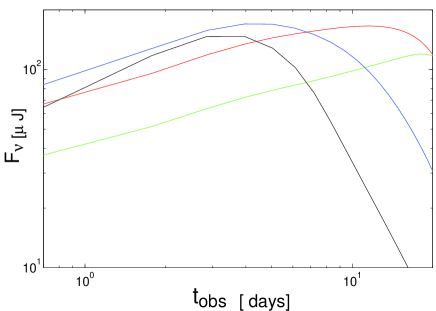
Figure 6: The green, red, blue and black curves represent the light curves at the observed frequencies $10^{8},10^{9},10^{10}$ and $10^{11}\ {\rm Hz}$, respectively, as seen by an observer at a distance of $10^{28}\ {\rm cm}$ along the jet axis.

References

- (1) Blandford, R.D. & McKee, C.F. 1976, Phys. of fluids, 19, 1130.
- (2) Granot, J, Piran, T. & Sari, R. 1999, ApJ, 513, 679.
- (3) Rhoads, J.E., 1999, ApJ submitted, astro-ph9903399.
- (4) Sari, R., Piran, T. & Halpren, J.P., 1999, ApJ, 519, L17.
- (5) Wei, D.M. & Lu, T. 1999, astro-ph9908273