Using Perturbative Least Action to Recover Cosmological Initial Conditions

Abstract

We introduce a new method for generating initial conditions consistent with highly nonlinear observations of density and velocity fields. Using a variant of the Least Action method, called Perturbative Least Action (PLA), we show that it is possible to generate several different sets of initial conditions, each of which will satisfy a set of highly nonlinear observational constraints at the present day. We then discuss a code written to test and apply this method and present the results of several simulations.

1 Introduction

What initial density fluctuations gave rise to the present day structure in the universe? We have a number of reasons for asking this question. First, generating consistent initial conditions for observations on small scale would give us a means of extracting the small-scale primordial power spectrum, which can, for example, be used to constrain the neutrino mass (Hu, Eisenstein & Tegmark 1998). In addition, many dynamic systems of interest such as groups and clusters can be tested for consistency with cosmological models by determining what initial conditions could give rise to them within a given scenario. Finally, initial conditions which will evolve to satisfy known constraints at the present day can be useful as input to numerical simulations that study the evolution of galaxies and clusters.

If the primordial fluctuations were Gaussian, then the power spectrum on large scale ($\gtrsim 10$ Mpc) today fully characterizes the statistical properties of the cosmological density field (e.g. Peebles 1980 §10 and references therein). Any linear field can be uniquely time-reversed to provide an initial density field at high redshift. A linear field is one which, when smoothed on sufficiently large scales, gives a standard deviation of density perturbations, $\delta(({\bf x},t_{0})\equiv\rho({\bf x},t)/\overline{\rho}(t_{0})-1$, of less than unity, where $t$ is the physical time, $t_{0}$ is time at $z=0$, and where ${\bf x}$ is a position in space in comoving coordinates. When density fluctuations are small, linear perturbation theory yields the following simple relationship between an observed distribution at the present and at high redshifts:

$$\delta({\bf x},t_{i})=\frac{D(t_{i})}{D(t_{0})}\delta({\bf x},t_{0})\ ,$$ (1)

where the linear growth factor at present, $D(t_{0})$ is normally set to unity.

The problem of determining initial conditions for highly nonlinear final density fields is a much more complex problem. Due to mode-mode coupling in the evolution equations (see e.g. Peebles 1980 §18), time-reversal of a set of orbits becomes fundamentally ill-posed; that is, many different sets of initial conditions can give rise to the same or similar final density fields. In an N-body simulation, this can be thought of in terms of the trajectory of particles crossing one another. Since a region of large overdensity is populated by many particles originating elsewhere, assigning particles uniquely to their point of origin becomes impossible.

In this paper, we will develop a method for dealing with the problem of time-reversing highly non-linear gravitational dynamic systems in a realistic physical context. The basic goal throughout will be as follows: given some observed or target density field, $\delta({\bf x},t_{0})$ or a set of target constraints, such as density peaks or voids in particular places, how does one go about generating one or more sets of initial conditions, $\delta({\bf x},t_{i})$, which, when run through a gravity code, will yield the desired final conditions?

In order to answer this question, in §2 we will describe generic methods for going from general constraints to constraints on trajectories of individual particles. We will further discuss some of the methods that other researchers have used to try to satisfy those constraints and generate initial conditions. In §3, we discuss one of the most promising methods, Least Action analysis, which gives a single correct, but not necessarily physically well motivated, set of initial conditions. In §4, we will describe Perturbative Least Action (PLA), which allows one to generate well motivated initial conditions by perturbing random realizations of a known initial power spectrum. In addition, we will discuss a set of codes which have been written in order to apply PLA to some test fields. In §5, we will show the results of two groups of toy problems used to test the PLA code. Finally, in §6, we will consider future applications.

2 The Cosmological Constrained Boundary Problem

2.1 Initial Conditions: The Zel’dovich Approximation

In the standard cosmological model, perturbations in the density field at the present day arose out of a nearly uniform field at early times. Rather than treat the density field as a continuum, it is convenient to think of the matter in the universe as a distribution of particles which may be binned and smoothed in order to yield a density field. Of course, the positions and velocities of those particles may be evolved using any of the standard N-body techniques (e.g. Hockney & Eastwood 1981, and references therein).

At very early times, the particle field deviates little from a uniform grid. For convenience, we will use the notation, ${\bf q}_{i}$ to denote the positions of particles on the grid, and ${\bf d}_{i}(t_{i})\equiv{\bf d}({\bf q}_{i},t_{i})$ to denote the displacement of each particle from its gridpoint as well as a vector field of the same. Thus, at $t=t_{i}$:

$${\bf x}_{i}(t_{i})={\bf q}_{i}+{\bf d}_{i}(t_{i})\ .$$ (2)

However, it may readily be shown that for small perturbations:

$$\delta({\bf x},t_{i})\propto-\nabla\cdot{\bf d}({\bf q}_{i},t_{i})\ .$$ (3)

But, as we pointed out earlier, small perturbations grow according to a linear growth factor. Thus:

$${\bf d}_{i}(t)=\frac{D(t)}{D(t_{i})}{\bf d}_{i}(t_{i})$$ (4)

as long as perturbations remain small. This is the well known Zel’dovich approximation (Zel’dovich 1970). In addition, since it may be shown that fields for which there is a curl in ${\bf d}({\bf q}_{i},t_{i})$ produce decaying modes and our preferred model contains only growing modes in the “linear” regime, we will always assume that ${\bf d}({\bf q}_{i},t_{i})$ may be expressed as the gradient of a scalar field.

2.2 Final Conditions: Matching a Set of Constraints

After a particle field has evolved via gravitational collapse, we may once again measure the corresponding density field, $\delta({\bf x},t_{0})$. However, since our concern in this exercise is ensuring that the density field satisfies some set of constraints, we will now discuss how to generate a particle field which satisfies density field constraints.

In most reconstruction schemes, the goal is to find the “true” initial conditions for some randomly selected region of the universe (e.g. Narayanan & Croft 1999 and references therein). Normally, tests of these methods consist in running an N-body simulation and attempting to match the initial conditions by examining the final conditions. For this, a particle field, $\tilde{\bf x}_{i}(t_{0})$, is laid down such that the smoothed density field of the particles yields the target density field. At this point, no consideration is given to where a particle started out. However, recall that at $a=0$ (where $a$ is the cosmological expansion factor, and $a(t_{0})\equiv 1$) particle $i$ necessarily sits at its gridpoint, ${\bf q}_{i}$. Since we do not want particles traveling inordinately far, and since the smoothed density density field will remain unchanged if we interchange the indices of two particles, it is general practice that particles will be interchanged until they have to move as far as possible. Thus, we find the permutation matrix ${\bf M}_{ij}$ such that

$$\Delta^{2}[{\bf M}_{ij}\tilde{\bf x}_{j}(t_{0}),{\bf q}_{i}]\equiv\sum_{i}\left[{\bf q}_{i}-{\bf M}_{ij}\tilde{\bf x}_{j}(t_{0})\right]^{2}$$ (5)

is minimized. This can be done, for example, using a simulated annealing method (Press et al. 1992).

We finally define

$${\bf x}_{i}(t_{0})={\bf M}_{ij}\tilde{\bf x}_{j}(t_{0})$$ (6)

as the final particle positions.

In addition to problems which constrain the entire density field, we are also interested in scenarios in which particular regions are constrained to have particular overdensities. We discuss this alternate set of constraints § 4.2.1.

2.3 Matching the Initial and Final Conditions

At this point, we have found an initial and final position for each particle. However, initial in this sense refers to the particle’s position at $a=0$. In a practical sense, we are interested in the particle’s position shortly thereafter. And it is this high-redshift position and velocity (coupled via the Zel’dovich approximation) which we shall henceforth refer to as the “initial conditions” of a particle field.

The Perturbative Least Action (PLA) has been developed in order to solve this problem in a new and physical well-motivated way. Narayanan & Croft (1999) discuss other attempts recover initial conditions, including linear theory, the Zel’dovich-Bernoulli Method (Nusser & Dekel 1992), Gaussianization (Weinberg 1992), and PIZA (Croft & Gaztañaga 1997), which they show as most accurately reproducing the initial conditions. PIZA essentially sets the initial offsets of the particles as:

$${\bf d}_{i}(t_{i})=D(t_{i})\left[{\bf x}_{i}(t_{0})-{\bf q_{i}}\right]\ ,$$ (7)

with a corresponding velocity given by the Zel’dovich approximation.

3 Ordinary Least Action

Another reconstruction scheme which has received a great deal of attention is the Least Action approach (Peebles 1980 §20, 1989, 1993, 1994, Shaya, Peebles & Tully 1995). It is from these examples that we will make our foray into Perturbative Least Action, and therefore we will discuss this method in some detail.

The idea of Least Action is that, given a set of boundary constraints, such as the initial and final positions of each particle, for example, or the initial position, and the final angle and radial velocity, one can determine the set of orbits of particles by finding the trajectories that extremize the action, defined as the time integral of the Lagrangian.

In a cosmological context, the Lagrangian of a particle, $i$, can be expressed as:

$${\cal L}_{i}=m_{i}\frac{{\bf u}_{i}^{2}}{2}-m_{i}\Phi_{i}\ ,$$ (8)

where ${\bf u}_{i}\equiv\partial(a{\bf x)}_{i}/\partial t$ and $\Phi_{i}$ is the total potential (background plus perturbations) at the position of particle $i$. We will henceforth assume that the mass, $m_{i}$, is the same for all particles, and for convenience, we will units in which $m_{i}=1$. By subtracting out the Lagrangian of a particle in a homogeneous universe (see, e.g. Peebles 1980 §7 for a derivation), the Lagrangian reduces to:

$${\cal L}_{i}=\frac{a^{2}\dot{\bf x}_{i}^{2}}{2}-\phi_{i}\ ,$$ (9)

where $\phi_{i}$ is the potential felt by particle $i$ due to the density perturbations alone, and is equal to zero in an infinite, smooth density field.

The cosmological Least Action variational principle states that a set of particles, each traveling between two known points, will each take the path which locally extremizes the action, defined as:

$$S\equiv\sum_{i}\int_{0}^{t_{0}}dt\ {\cal L}_{i}=\sum_{i}\int dt\left(\frac{a^{2}\dot{\bf x}_{i}^{2}}{2}-\frac{\phi_{i}}{2}\right)\ ,$$ (10)

From now on, we will dispense with limits on the time integrals since all of them are implicitly from $t=0$ to $t=t_{0}$.

Though any extremum (minimum, maximum, or inflection point) will yield physically viable orbits, it is numerically most stable to find the set of orbits which locally produces the least action, which is the approach and terminology we will use henceforth.

In the case of discrete point sources:

$$\phi_{i}\equiv\sum_{j}\phi_{ji}=\sum_{j}\frac{Gm_{i}m_{j}}{r_{ij}}$$ (11)

Since $\phi_{ij}=\phi_{ji}$ (as all masses are identical), the total binding energy of the system is expressed as $\sum_{i}\phi_{i}/2$.

In order to minimize the action, we express each particle trajectory as a linear combination of a set of basis functions, and then minimize the action with respect to these coefficients:

$${\bf x}_{i}(t)={\bf q}_{i}+f_{0}(t)\left[{\bf x}_{i}(t_{0})-{\bf q}_{i}\right]+\sum_{n=1}^{n_{max}}{\bf C}_{i,n}f_{n}(t)$$ (12)

where we have defined $f_{n=0,n_{max}}(0)=0$, $f_{0}(t_{0})=1$, $f_{n=1,n_{max}}(t_{0})=0$, and $a^{2}\dot{f}_{n=0,n_{max}}(t)\rightarrow 0$ as $a\rightarrow 0$. A good solution for the zeroth basis function gives $f_{0}(t)=D(t)$. Using these constraints, the Zel’dovich approximation is necessarily satisfied for each basis function, and hence, for each particle trajectory at early times.

The Least Action principle demands that given a physical set of orbits, all derivatives of $S$ with respect to ${\bf C}_{i,n}$ will vanish. Thus:

$$\nabla_{{\bf C}_{i,n}}S=\int dt\left[\dot{f}_{n}(t)a^{2}\dot{\bf x}_{i}-f_{n}(t)\nabla\phi_{i}\right]=0\ ,$$ (13)

where here and throughout, unlabeled gradients are assumed to be with respect to the comoving coordinate system. By using the constraints listed above and doing an integration by parts, this is algebraically equivalent to:

$$\nabla_{{\bf C}_{i,n}}S=\int dtf_{n}(t)\left[-\frac{\partial}{\partial t}(a^{2}{\bf\dot{x}})+\nabla\phi_{i}\right]=0\ .$$ (14)

However, everything inside the parentheses on the right side of the equation necessarily equals zero (as must its time integral) if the equations of motion are satisfied, as it is merely Newton’s second law written in comoving coordinates. By using the form of the trajectory in equation (12), we find a set of orbits which necessarily satisfies both the equations of motion and the constraints, and will converge quickly.

Since the evolution equations are implicitly dependent upon the underlying cosmology, examination of the velocities of galaxies can potentially give limits on cosmological parameters. This approach has been applied, for example, to galaxies within 3000 km/s (Shaya, Peebles and Tully 1995; Dunn & Laflamme 1995), yielding a value of $\Omega_{m}\simeq 0.2$. Branchini & Carlberg (1995), on the other hand, argue that Least Action analysis dramatically underestimates $\Omega_{m}$, and that Local Group dynamics could yield a value as high as $\Omega_{m}=1$.

In general, the ordinary Least Action approaches use direct particle-particle summation to calculate the forces on particles. We use a particle mesh (PM) Poisson solver to compute forces, which greatly speeds up computation. A similar approach to ordinary Least Action was used by Nusser and Branchini (1999) who used a tree code scheme to compute particle forces.

While ordinary Least Action analyses provide physically correct orbits for particles, the initial conditions found need not have any resemblance to a field drawn from an a priori known power spectrum. Rather, particle trajectories have traditionally been generated which evolve a field from a completely uniform one to one satisfying the constraints using the least total distance for each particle, as is the case with the PIZA algorithm. In addition, the actual path of the particles given by direct application of Least Action (as well as linear perturbation theory or PIZA) essentially gives a first infall solution, rather than allowing for the possibility of orbit crossings. Moreover, nothing in the generation of initial conditions demands that the initial fields be curl-free; thus, decaying modes can develop.

4 Method: Perturbative Least Action

In order to alleviate these problems inherent in ordinary Least Action, we now develop a method to generate an ensemble of initial conditions, each as consistent as the constraints will allow with a specified primordial power spectrum. In this section we will first develop the equations governing PLA. We will then discuss the background cosmology and numerical methods in our code. Next, we will discuss the various types of target density fields to be used in our simulations. We will then discuss how basis functions are generated. Finally, we will explain how the perturbed action is minimized using the PLA code.

4.1 General Equations

First, let us suppose that we have run an N-body code on a randomly generated some set of initial conditions with known power spectrum. The path of each particle, $\{{\bf x}^{(0)}_{i}(t)\}$, is known to satisfy the cosmological equations of motion. Let us, by perturbing around the final “unperturbed” density field, find a set of ${\bf x}_{i}(t_{0})$ which produce a density field satisfying our constraints on the system. The full path of each particle can be expressed as a perturbation around ${\bf x}_{i}^{(0)}(t)$ using the basis functions introduced above. Thus, we may say:

$${\bf x}_{i}(t)={\bf x}_{i}^{(0)}(t)+f_{0}(t){\bf x}^{(1)}_{i}(t_{0})+\sum_{n=1}^{n_{max}}{\bf C}_{i,n}f_{n}(t)$$ (15)

where we have applied the same constraints on $f_{n}(t)$ as discussed above, and ${\bf x}^{(1)}_{i}(t)$ is the perturbation orbit such that ${\bf x}_{i}^{(1)}\equiv{\bf x}_{i}-{\bf x}_{i}^{(0)}$. Comparison of this equation with equation (12) illustrates that Least Action and PLA are quite similar, but perturb around different guesses for the particle trajectory.

Since for highly nonlinear systems, there may be many minima of the action which produce the correct final conditions, by perturbing away from a known field which is consistent with a given power spectrum, we are able to keep each realization as physically relevant as possible, and find the “closest” local minimum in parameter space.

We may now rewrite the action (equation 10) as,

$$S = \sum_{i}\int_{0}^{t_{0}}dt\left(\frac{a^{2}\dot{\bf x}^{(0)2}_{i}}{2}-\frac{\phi^{(0)}_{i}}{2}\right)+\sum_{i}\int_{0}^{t_{0}}dt\left(a^{2}\dot{\bf x}_{i}^{(0)}\cdot\dot{\bf x}_{i}^{(1)}+\frac{a^{2}\dot{\bf x}^{(1)2}_{i}}{2}-\frac{\phi_{i}}{2}+\frac{\phi^{(0)}_{i}}{2}\right)$$ (16)

$$= S^{(0)}+\sum_{i}\int_{0}^{t_{0}}dt\left(a^{2}\dot{\bf x}_{i}^{(0)}\cdot\dot{\bf x}_{i}^{(1)}+\frac{a^{2}\dot{\bf x}^{(1)2}_{i}}{2}-\frac{\phi_{i}}{2}+\frac{\phi^{(0)}_{i}}{2}\right)\ ,$$

where $\phi^{(0)}_{i}$ is the potential on particle, $i$, in the unperturbed, (${\bf x^{(0)}}$), potential field.

The gradient of the action with respect to the coefficients is:

$$\nabla_{{\bf C}_{i,n}}S=\int dt\left[\dot{f}_{n}(t)a^{2}\left(\dot{\bf x}^{(0)}+\dot{\bf x}^{(1)}\right)-f_{n}\nabla\phi_{i}\right]$$ (17)

However, by definition,

$$\int dt\left[\dot{f}_{n}(t)a^{2}\dot{\bf x}^{(0)}_{i}-f_{n}(t)\nabla\phi^{(0)}_{i}\right]=0\ ,$$ (18)

so,

$$\nabla_{{\bf C}_{i,n}}S=\int dt\left[\dot{f}_{n}(t)a^{2}\dot{\bf x}^{(1)}+f_{n}\left(\nabla\phi^{(0)}_{i}-\nabla\phi_{i}\right)\right]$$ (19)

It is also often useful to calculate the Hessian Matrix of second derivatives in order to minimize the action:

$${\cal H}_{i\alpha\beta,nm}\equiv\frac{\partial^{2}S}{\partial C_{in}^{\alpha}\partial C_{jm}^{\beta}}=\int dt\left[a^{2}\dot{f}_{n}\dot{f}_{m}\delta_{ij}\delta_{\alpha\beta}-f_{n}f_{m}\frac{\partial^{2}\phi_{i}}{\partial x_{i}^{\alpha}\partial x_{j}^{\beta}}\right]\ ,$$ (20)

where $\alpha$ and $\beta$ are direction indices. We will discuss application of the Hessian matrix for minimization in § 4.2.3.

4.2 The PLA Procedure

In this section, we describe how PLA is actually applied in practice. We begin the process by running an N-body simulation with a random seed. These trajectories will be referred to as ${\bf x}_{i}^{(0)}(t)$. In our simulations, we use a Particle Mesh (PM) code (Hockney & Eastwood 1981). Though the power spectrum and cosmology of the unperturbed simulation is held to be constant in the following simulations, in a forthcoming paper, we will show how PLA may be used to discriminate between different cosmological models.

4.2.1 The Target Density Field

After we run the unperturbed simulation, we must next figure out what perturbations need to be applied to the particle paths at $t=t_{0}$. This may be done in any way, may satisfy any sort of constraint, and the details of determining the final positions of the perturbed orbits are not crucial to the PLA method itself. However, since some perturbations will be easier to satisfy than others, we will briefly discuss the method used in our code to perturb the particle trajectories. We will thus discuss means of generating a target density field, $\delta({\bf x},t_{0})$, from the smoothed density field of the unperturbed simulation, $\delta^{(0)}({\bf x},t_{0})$.

In § 2.2, we discussed the traditional method of generating a target field: running a numerical simulation with a different random seed than our unperturbed field. However, the PLA approach was originally formulated with the intent of providing initial conditions to highly nonlinear individual constraints, such as rich clusters appearing in particular regions, or large voids appearing elsewhere. We will now discuss how to generate a “realistic” target density field which constrains the mean final overdensity in particular regions, which resembles the unperturbed simulation as closely as possible.

To this end, we use a very similar approach to the “Constrained Initial Conditions” method employed by Hoffman & Ribak (1991, 1992), and pioneered by Bertschinger (1987). While Constrained Initial Conditions are actually meant to provide initial conditions on large scales (linear at the present day), as a side effect, it can be used to map one (even highly nonlinear) density field onto another while satisfying a set of given constraints and at the same time preserving the autocorrelation of the density field.

While objections might certainly be made that the Constrained Initial Conditions method makes assumptions about the statistical properties of the density field to be generated (such as that it is Gaussian random) which may not hold in the nonlinear regime, we re-iterate that we have chosen this method for generating a final target field because it is convenient, but not intrinsic to the PLA method, itself.

In order to create a “target” density field (the field which will both satisfy the given constraints and has the same large scale distribution as the unperturbed field), we begin by computing a gridded density field, using a Cloud-In-Cell (CIC) interpolation scheme (Hockney & Eastwood 1981). Next, we calculate the autocorrelation function $\xi^{(0)}(r)$ of the unperturbed field, $\delta^{(0)}({\bf x},t_{0})$.

We define our constraints such that within some region, ${\cal R}_{n}$ (defined as a normalized tophat function), we want to have some given mean, $\overline{\delta}({\cal R}_{n},t_{0})=c_{n}$. Following the prescription of Hoffman & Ribak, we next compute the correlation of each constraint with every point on the density field:

$$\xi^{(0)}_{n}({\bf r})=\int d^{3}{\bf r}^{\prime}\xi^{(0)}(|{\bf r}-{\bf r}^{\prime}|)\delta^{D}({\bf r}^{\prime}-{\cal R}_{n})$$ (21)

In addition, we need to compute the correlation between each constraint:

$$\xi^{(0)}_{nm}=\xi^{(0)}_{mn}=\int d^{3}{\bf r}\xi^{(0)}_{n}({\bf r})\delta^{D}({\bf r}^{\prime}-{\cal R}_{m})$$ (22)

We then constrain the density field by applying the relation:

$$\tilde{\delta}({\bf x},t_{0})=\delta^{(0)}({\bf x},t_{0})+\xi^{(0)}_{n}({\bf r})\xi^{-1}_{nm}(c_{m}-c^{(0)}_{m})\ .$$ (23)

At this point, we choose to regularize our solution. We have found it practical to demand that the initial power spectrum of the field remain unchanged on perturbation. We thus apply a correction to the initial perturbed field such that

$$\delta({\bf k},t_{0})=\tilde{\delta}({\bf k},t_{0})\sqrt{\frac{P^{(0)}(k)}{\tilde{P}(k)}}\ .$$ (24)

This necessarily insures that the final density fields have the same power spectrum, and generally only makes a correction at large scales where linear theory would be expected to hold. Others may choose to add different forms of regularization to their simulations. The choice is not intrinsic to PLA, itself.

We may also compute a target density field by simply taking the observed density field from another simulation, as we will do in the second set of simulations.

Once the target density field has been computed and particle positions are determined which satisfy this field, it remains only to calculate the permutation matrix, ${\bf M}_{ij}$ in order to have a set of final constraints. We may use the basic procedure discussed in § 2.2, with one small adjustment. Rather than finding a permutation matrix that minimizes offsets from the uniform grid, in PLA we want to minimize $\Delta^{2}[{\bf M}_{ij}\tilde{\bf x}_{j}(t_{0}),{\bf x}^{(0)}_{i}(t_{0})$]. Recall

$${\bf x}_{i}(t_{0})={\bf M}_{ij}\tilde{\bf x}_{j}(t_{0})\ ,$$ (25)

and

$${\bf x}^{(1)}_{i}(t_{0})={\bf x}_{i}(t_{0})-{\bf x}^{(0)}_{i}(t_{0})\ .$$ (26)

We have thus generated the sought-after perturbations for the final particle field.

4.2.2 Basis Functions

Once we have generated unperturbed and perturbed positions, we next run the PLA code which will determine initial conditions which will give rise to the perturbed field.

The first step in this code is determination of appropriate basis functions. A natural choice is that all basis functions should be polynomials with base $D(t)$, since we know that lower order perturbation theory will yield solutions of this form. Earlier, we said that $f_{0}=D(t)$. Likewise, we set: $f_{1}=D(t)\left[1-D(t)\right]$.

For higher order basis functions, we examine the unperturbed trajectories, and successively create best fit basis function (polynomials which best fit the residuals of the unperturbed trajectories) of the form:

$$f_{n}=\sum_{m=n}^{m_{max}}b_{nm}D(t)^{m}\left[D_{0}-D(t)\right]\ ,$$ (27)

where the kernel polynomials are the same form used by Giavalisco et al. (1993).

Given the form of the coefficients, only $f_{0}$ and $f_{1}$ grow linearly at early times, and hence, the corresponding coefficients are those which are used to generate the initial conditions.

4.2.3 Determining the Coefficients

We are now prepared to compute the coefficients which minimize the action. Because of the form of the interpolation scheme for the potential in PM codes, computation of the actual potential, itself, rather than its spatial derivatives is not well defined. Hence, when we minimize the action we actually want to find coefficients such that the derivatives of the action (equation 19) vanish.

In order to do this, we assume that each particle and direction are approximately independent of one another, and that the strongest correlations will be between different coefficients of the same particle. Our minimization scheme is similar to the Levenberg-Marquardt Method (Press et al. 1992, §15.5), and uses the inverse of the Hessian matrix to compute the steps in coefficients:

$$\Delta C^{\alpha}_{i,n}=-\sum_{m=1}^{n_{coeff}}\frac{\partial S}{\partial C^{\alpha}_{i,m}}{\cal H}^{-1}_{i\alpha\alpha,mn}\ .$$ (28)

In addition to minimizing the action, we wish to put a constraint on our trajectories that they only have a growing mode at early times. Consistent with that is our assumption that our initial velocity field be curl free. In order to insure this, we must confine ${\bf C}_{i,1}$ to a submanifold such that

$$\nabla_{\bf q}\times{\bf C}_{i,1}=\nabla_{\bf q}\times{\bf\Delta C}_{i,1}=0\ .$$ (29)

Recall that of the basis functions, only the first grows linearly at early times, and hence, at high redshift, the velocity field will be given by the first coefficients. Further recall that at early times, the positions of particle, $i$, is approximately given by ${\bf q}_{i}$, allowing us to take spatial derivatives of the velocity field.

In order to make $\Delta{\bf C}_{i,1}$ curl-free, we take the Fourier transform of the initial estimate of the step (equation 28), and find a new Field such that $\Delta{\bf C}_{1}({\bf k})\propto{\bf k}$ everywhere, and the difference squared of the old and new field are minimized.

We then iterate until convergence is reached. At this point, the initial positions and velocities of the perturbed field are computed, and the initial density field is corrected to yield an identical power spectrum to that of the unperturbed field using equation (24). This new field may be plugged into an N-body code and will approximately yield ${\bf x}(t_{0})$.

Of course, if satisfactory convergence is not reached after one try, the results of the final N-body simulation may be used as the new unperturbed simulation, and the process may be repeated as needed.

5 The Simulations

In order to test the concept of the PLA method, we have run two groups of simulations. A discussion of the numerical method is presented in the previous section.

5.1 Test 1: Matching a Random Field

The first test of the PLA code is a natural choice for any code which tries to determine initial conditions; namely, given a density field from an N-body simulation, how well can the method compute the initial conditions. This is the test constructed by Narayanan & Croft (1999), in which they demonstrate the superiority of PIZA to other reconstruction schemes.

In our test, we run a randomly realized simulation with standard CDM cosmology ($\Omega_{0}=1.0$, $\Lambda=0.0$) on a grid with $64^{3}$ particles, $128^{3}$ gridcells, a gridlength of $100h^{-1}$ Mpc, and with $\sigma_{8}=1$, and compute the final density field. We then run another simulation with the same cosmology, which will be used for nothing more than generating an initial power spectrum. Objections might be raised that we have no a priori knowledge of the cosmology, and hence, have no right to do this. However, we will show in a forthcoming paper how one may use PLA to generate a maximum likelihood estimate of cosmological parameters. For now, we will assume such parameters are known (as they are assumed to be in Naryanan and Croft 1999).

From the target density field, we then compute a final particle field, ${\bf x}_{i}(t_{0})$, which both satisfies the density field, and minimizes $\Delta^{2}[{\bf q}_{i},{\bf x}_{i}(t_{0})]$. Note that we are perturbing away from a uniform field, rather than from the positions of a randomly generated simulation. From here, however, we apply the method exactly as described in § 4.

With this test we hope to examine two things: 1) How well are the actual initial conditions from the target field reproduced? 2) After running the generated initial conditions through the PM code, how well does the final density field match the final target density field?

Recall that as part of the method, we are constraining the initial power spectrum to match the “known” primordial power spectrum. In addition, our constraints guarantee that the field is necessarily curl free, and that the initial displacements satisfy the Zel’dovich approximation. Beyond that, a good statistical test of difference is given by Narayanan & Croft (1999), who define a difference of complex amplitudes between field “1” and “2” as:

$$D(k,t)=\frac{\sum[\delta_{1}({\bf k})-\delta_{2}({\bf k})]^{2}}{\sum[\delta_{1}({\bf k})^{2}+\delta_{2}({\bf k})]^{2}}\ ,$$ (30)

where $\delta_{1}({\bf k})$ and $\delta_{2}({\bf k})$ are the Fourier components of density field “1” and “2” respectively.

In Figure 1, we examine this statistic as a function of k for both the initial and final condition fields. We look at the difference between the target field and PIZA, and various numbers of iterations of PLA. This is intended to be almost identical to Figure 7 in Narayanan & Croft (1999), and illustrates that even with only one iteration, PLA fits both the initial and final target density field better than PIZA, which was shown to be the previous leading contender for initial condition reconstruction.

Figure 1: a) Comparison of the initial density fields generated using PIZA (solid line), and various iterations of PLA (dotted, short dashed, and long dashed lines for 1, 2, and 3 iterations, respectively), to the actual initial conditions used to generate a random target field. The density fields are Fourier decomposed, and the modes are compared according to the difference coefficient, $D(k)=\sum[\delta_{1}({\bf k})-\delta_{2}({\bf k})]/\sum[\delta_{1}({\bf k})^{2}+\delta_{2}({\bf k})^{2}]$. The nonlinear scale ($k=2\pi/16h^{-1}$ Mpc), is denoted by $k_{nl}$. b) A similar comparison, but for the evolved density fields.

With further iterations, the initial field stabilizes at a somewhat worse fit than the first iteration. This is not two surprising since the differences in fit occur exclusively on the nonlinear scale. Since a unique fit cannot to the final field cannot be found, and since the final field is ultimately what PLA tries to match, some phase mixing may cause a slightly worse fit in the initial field.

The final field, however, improves on one additional iteration, and then slightly worsens on a third. Thereafter, we’ve found the result more or less stabilizes. We have found, however, that we get a better fit on all physical scales for both the initial and final fields by running our simulations in a box in which the resolution scale is somewhat larger.

5.2 Test 2: Constraining Clusters

In our second set of simulations, we have tried to form three rich clusters in specified positions within a known field. We have run three randomly realized simulations with different random seeds. Each is run with a standard CDM cosmology ($\Omega_{0}=1.0$, $\Lambda=0.0$) on a grid with $64^{3}$ particles, $128^{3}$ gridcells, a gridlength of $100h^{-1}$ Mpc, and with $\sigma_{8}=1$. We then specify three positions, and demand that within a radius of $1.5h^{-1}$ Mpc of those positions, the mean overdensity become $\overline{\delta}=200$, giving us rich Abell clusters.

The general method for doing this is described in great detail in §4. In this test, we used 4 basis functions for each set of simulations, and typically ran four cycles (minimizing of the action, and re-running the new initial conditions in the PM code) until satisfactory convergence was reached.

As illustrated in Table 1 and 2, the results of this exercise are quite successful. In the figures, the integrated average density within the constraints regions is shown for the 3 unperturbed and perturbed realizations, respectively. Recall that both the perturbed and unperturbed realizations are the output of the running the perturbed and unperturbed initial conditions through a PM code.

Value of Constraints in Unperturbed Simulations
Cluster	$\overline{\delta}$ (model)	$\overline{\delta}$ (sim 1)	$\overline{\delta}$ (sim 2)	$\overline{\delta}$ (sim 3)
1	200	-0.41	-0.20	-0.83
2	200	-0.83	-0.99	-0.83
3	200	-0.98	0.06	-0.97

Table 1: A summary of how well the random realizations satisfy the constraints to be imposed. The constraints consist of a region of radius $1.5h^{-1}$ Mpc, with a mean overdensity of $\overline{\delta}=200$. If anything, the regions selected are voids in the unperturbed realizations.

Value of Constraints in Perturbed Simulations
Cluster	$\overline{\delta}$ (model)	$\overline{\delta}$ (sim 1)	$\overline{\delta}$ (sim 2)	$\overline{\delta}$ (sim 3)
1	200	201	189	141
2	200	155	176	215
3	200	206	226	191

Table 2: A summary of how well the evolved perturbed fields satisfy the imposed constraints at $z=0$. Note that the largest error in mass is $\sim 30\%$, and that a typical error is about 10%.

In addition to a strict evaluation of how well the constraints are satisfied, a visual inspection of the final density fields may also be instructive. In Figures 2-4 we show the density fields of the a) unperturbed and b) perturbed evolved density fields. As a reminder, both are the result of actually running an initial field through the PM code. The plots show contours of regions with overdensities of greater than 50 smoothed on a scale of $1.5h^{-1}$ Mpc. Note that though a number of the “clusters” remain virtually unchanged through the perturbation, our rich target clusters appear precisely on target in all three realizations.

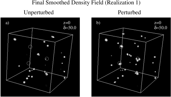
Figure 2: Realization 1. a) A plot the smoothed ($r=3h^{-1}$Mpc) density field, showing contours of $\delta=50$ for the first unperturbed realization. b) A similar plot, showing the evolved density field of the perturbed simulations. The circles in each indicate the location of the target clusters.

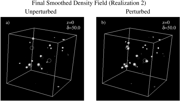
Figure 3: Realization 2. As in Fig. 2, but for the second realization.

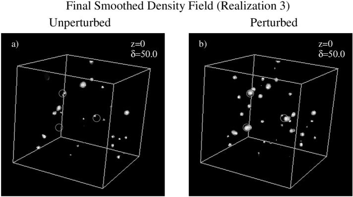
Figure 4: Realization 2. As in Fig. 2, but for the third realization.

Finally, we may consider a measure of how much a field needs to be perturbed in order that it might satisfy the constraints. In Figure 5, we show the Fourier Difference statistic of a) the three combinations of pairs of perturbed initial density fields generated by PLA in this test, and b) the difference between the perturbed and unperturbed initial conditions for the three realizations. Note that on all scales the three different realizations are completely uncorrelated (up to cosmic variance). However, on large and intermediate scales, the initial conditions maintain much of their original structure.

Figure 5: The Fourier Difference squared statistic for various combinations of initial fields in test 1. a) The three pairs of perturbed density fields are completely uncorrelated with one-another. b) Down to even mildly nonlinear scales, the perturbed and unperturbed initial density fields have a very high correlation.

5.2.1 A High-Resolution Realization

One of the great benefits of PLA is that once initial conditions have been generated which satisfy a set of constraints, the field may be Fourier decomposed, and large $k$ modes may be filled in using a known primordial spectrum. This new initial field will have higher resolution than the original, and yet will reproduce all of the same features on larger scales. We have done this with the results of the first realization in test 2, using $128^{3}$ particles and $256^{3}$ grid cells. The results are shown in Figure 6.

After running the high resolution initial conditions through the PM code, the constraints are still satisfied to a tremendous degree, with the three overdensities measuring $\overline{\delta}=$175, 195, & 206, respectively. In this respect, the consistency of the high- and low-resolution simulations is quite telling. Moreover, visual inspection of the normal and high-resolution perturbed initial conditions yield virtually identical results when smoothed on the same scale. In Figure 6, we show a comparison of the $\delta=50$ density contour of the two different resolutions, each smoothed at $r=3h^{-1}$ Mpc. The two fields appear almost identical, suggesting that PLA is a viable technique for generating clusters in specified positions, and then using those initial conditions as a seed for a high-resolution study of the clusters.

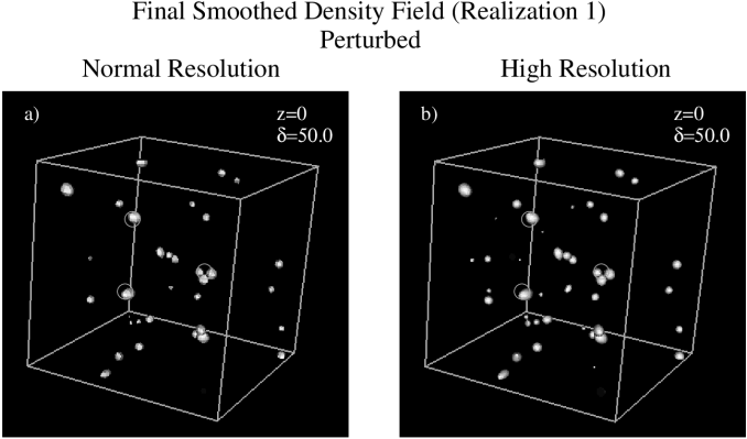
Figure 6: A comparison of the the first realization run at a) normal resolution, and b) high-resolution simulation, with small scale modes filled in with known power spectrum. The density contours and smoothing scale are as in Fig. 2.

6 Future Goals

This paper has largely concentrated on the method of using Perturbative Least Action to generate initial conditions, and as a proof of concept, we have generated initial conditions which beat PIZA in its ability both to reproduce an initial density field and to match a final density field.

In addition to the basic method discussed here, future implementations of the code will also incorporate redshift survey observations as well as the potential for using an external, linearly evolving, tidal field. This will be extremely useful in studying semi-isolated systems such as the Local Group of galaxies. By modeling the Virgo Cluster and the Great Attractor as perturbations on the local potential field, we can realistically generate initial conditions and model this system. From there, we could ask meaningful questions about infall history, dwarf galaxy statistics and so on. Moreover, we will have generated an initial density field which could be used as a testbed for various N-body codes. Finally, studies, such as those done by Peebles (1989) based on the timing of the local group, could be reproduced with extended halos in order to address the concerns voiced by Branchini & Carlberg (1995).

In the context of the Local Group, we will use PLA to explore cosmological parameter space. Basically, by running different simulations with different cosmological parameters, and finding those “Local Groups” which best reproduce the statistical properties and velocity field of the “Local Group”, we will be able to independently estimate the true underlying cosmology.

In addition to highly nonlinear fields, we can use PLA to model quasi-linear fields such as those observed in the IRAS survey. An initial power spectrum could then be generated which could be compared to those produced using perturbation theory. While groups have investigated the evolution of the power spectrum using perturbation theory (e.g. Jain & Bertschinger 1994), PLA essentially evolves the power spectrum to all orders, and moreover, preserves phase information. Using this approach, we will get a much stronger handle on the primordial power spectrum on small scales.

Finally, in this paper we have described the case in which we have observations constraining the final density distribution. For a redshift survey, however, one has a three-dimensional density field in redshift space. Giavalisco et al. (1993) point out that this can be handled by performing a canonical transform on the basis functions. Future implementations of the code will constrain the density field in either real or redshift space.

References

- (1)
- (2) Bertschinger, E. 1987, ApJ, 323, 103L
- (3)
- (4) Branchini, E. & Carlberg, R.E. 1995 MmSAI 66, 219
- (5)
- (6) Croft, R.A.C. & Gaztañaga, E. 1997, MNRAS, 285, 793
- (7)
- (8) Dunn, A.M. & Laflamme, R. 1995 ApJ 443,1L
- (9)
- (10) Giavalisco, M., Mancinelli, B., Mancinelli, P.J., & Yahil, A. 1993, ApJ, 411, 9
- (11)
- (12) Hockney, R.W. & Eastwood, J.W. 1981, “Computer Simulations Using Particles” (New York: McGraw Hill)
- (13)
- (14) Hoffman, Y. & Ribak, E. 1991, ApJ, 380,L5
- (15)
- (16) Hoffman, Y. & Ribak, E. 1992, ApJ, 394, 448
- (17)
- (18) Hu, W., Eisenstein, D., & Tegmark, M. PRL 1998, 80, 5255
- (19)
- (20) Jain, B. & Bertschinger, E. 1994, ApJ, 431, 495
- (21)
- (22) Narayanan, V.K. & Croft, R.A.C. 1999, ApJ 515, 471
- (23)
- (24) Nusser, A. & Branchini, E. 1999 astro-ph/9908167
- (25)
- (26) Nusser, A. & Dekel, A. 1992, ApJ, 391, 443
- (27)
- (28) Peebles, P. J. E. 1980, “The Large-Scale Structure of the Universe” (Princeton: Princeton University Press)
- (29)
- (30) Peebles, P.J.E. 1989, ApJ, 344,L53
- (31)
- (32) Peebles, P.J.E. 1993, “Principles of Physical Cosmology” (Princeton: Princeton University Press)
- (33)
- (34) Peebles, P.J.E. 1994, ApJ, 429, 43
- (35)
- (36) Press, W.H., Teukolsky, S.A., Vetterling, W.T., & Flannery, B.P. 1992 “Numerical Recipes: The Art of Scientific Computing” (Cambridge, England: Cambridge University Press)
- (37)
- (38) Shaya, E.J., Peebles, P.J.E., & Tully, R.B. 1995, ApJS 454, 15
- (39)
- (40) Weinberg, D.H. 1992, MNRAS, 254, 315
- (41)
- (42) Zel’dovich, Y.B. 1970, A&A, 5, 84
- (43)