CMB Anisotropy in Compact Hyperbolic Universes II: COBE Maps and Limits

Abstract

The measurements of CMB anisotropy have opened up a window for probing the global topology of the universe on length scales comparable to, and even beyond, the Hubble radius. For compact topologies, the two main effects on the CMB are: (1) the breaking of statistical isotropy in characteristic patterns determined by the photon geodesic structure of the manifold and (2) an infrared cutoff in the power spectrum of perturbations imposed by the finite spatial extent. We calculate the CMB anisotropy in compact hyperbolic universe models using the regularized method of images [1, 2] described in detail in paper-I [3], including the line-of-sight “integrated Sachs-Wolfe” effect [2], as well as the last-scattering surface terms [1]. We calculate the Bayesian probabilities for a selection of models by confronting our theoretical pixel-pixel temperature correlation functions with the cobe–dmr data. Our results demonstrate that strong constraints on compactness arise: if the universe is small compared to the ‘horizon’ size, correlations appear in the maps that are irreconcilable with the observations. This conclusion is qualitatively insensitive to the matter content of the universe, in particular, the presence of a cosmological constant. If the universe is of comparable size to the ’horizon’, the likelihood function is very dependent upon orientation of the manifold wrt the sky. While most orientations may be strongly ruled out, it sometimes happens that for a specific orientation the predicted correlation patterns are preferred over those for the conventional infinite models. The full Bayesian analysis we use is the most complete statistical test that can be done on the COBE maps, taking into account all possible signals and their variances in the theoretical skies, in particular the high degree of anisotropic correlation that can exist. We also show that standard visual measures for comparing theoretical predictions with the data such as the isotropized power spectrum $C_{\ell}$ are not so useful in small compact spaces because of enhanced cosmic variance associated with the breakdown of statistical isotropy.

I Introduction

The cosmic microwave background anisotropy is currently the most promising observational probe of the global spatial structure of the universe on length scales near to and even somewhat beyond the ‘horizon’ scale ($\sim cH_{0}^{-1}$). As suggested by the concept of inflation, this relatively smooth Hubble volume that we observe is perhaps a tiny patch of an extremely inhomogeneous and complex spatial manifold. The complexity could involve non-trivial topology (multiple connectivity) on these ultra-large scales. Within a general program to address the observability of such a diverse global structure, a more well defined and tractable path would be to restrict oneself to spaces of uniform curvature (locally homogeneous and isotropic FRW models) but with non-trivial topology; in particular, compact spaces which have additional theoretical motivation [4, 5, 6, 7, 8]. For Euclidean (uniform zero curvature) or hyperbolic (uniform negative curvature) geometry, compactness necessarily implies non-trivial topology. Much recent astrophysical data suggest the cosmological density parameter in matter is subcritical [9], $\Omega_{m}<1$. Recently the presence of a significant cosmological constant (or, more generally, an exotic smooth component of matter) has been indicated by the high redshift supernova searches [10] and in studies combining large and intermediate angle CMB anistropy data with observations of cluster abundances and large scale galaxy clustering [11]. If this component does not compensate for the deficit from unity, $\Omega_{0}=\Omega_{m}+\Omega_{\Lambda}<1$, this would imply a hyperbolic spatial geometry for the universe; the additional requirement of compactness then ushers into consideration topologically compact hyperbolic (CH) universes, a field much richer in possibilities than the compact spaces with flat geometry when $\Omega_{0}$ is exactly unity.

In a universe with non-trivial global spatial topology, the multiple connectivity of the space could lead to observable characteristic angular correlation patterns in the CMB anisotropy arising directly from multiple imaging of the source terms that give rise to the anisotropy in the CMB. Moreover, the modified structure of the eigenmodes in such spaces implies that angular correlations would differ from the predictions in the simply connected space with identical geometry (the latter plays the role of the universal cover of the multiply connected space), even in the absence of multiple imaging of the sources. In particular, compact universes cannot support modes whose characteristic length scale exceeds the linear size of the space; consequently, the inferred power of fluctuations in compact models at large scales would appear suppressed relative to the power on the universal covering space. A more subtle effect is the angular dependence of the theoretical temperature variance which reflects generic inhomogeneity in the topologically compact spaces.

Paper-I [3] describes the regularized method of images, a general technique that we developed [1, 2] for computing the spatial correlations in a universe with non-trivial topology. In this paper we shall apply the method to calculate the angular correlation of CMB anisotropies in CH universe models. The angular correlation between the CMB temperature fluctuations in two directions in the sky completely encodes the CMB anisotropy predictions of any model that postulates Gaussian primordial fluctuations. Using the full correlation function information on the cobe–dmr data, we have obtained limits on the size of flat torus universe models that are a factor of two sharper than obtained from the angular power spectrum alone [12]. The main result was that the volume of the compact universe is constrained to be comparable to or larger than that of the observable universe. In [1], we proposed on the basis of simple arguments that compact universes with hyperbolic geometry should be expected to respect similar constraints. We have now carried out the full Bayesian analysis on accurate CMB correlation predictions in a large selection of CH universes and can demonstrate that essential features of our general constraint is borne out. In this paper we describe the details of our CMB correlation computation, highlight the general correlation features in the compact spaces, describe the method of comparison to data and present the resulting constraints from cobe–dmr using the examples of a large and a small CH universe. A compilation of our constraints on the flat torus models and a large selection of CH models will be presented in a separate publication [13].

The outline of this paper is as follows: In $\S$II we recapitulate that the angular correlation function of CMB anisotropy on large angular scales, that predominantly arises through both surface and integrated Sachs-Wolfe effects, can be related to spatial correlations of the gravitational potential on the three-space hypersurface at the epoch of last scattering. This is a useful simplification in terms of computational costs for calculating the CMB correlation in compact spaces using our method. Although we restrict our calculations here to large angular scales, Appendix A discusses the implementation of the method of images to calculate the CMB anisotropies at smaller angular scales. In $\S$III, we describe the computation of the angular correlation function of CMB anisotropy in CH models. The section also includes a quick review of some useful notions about compact spaces and the main result describing the regularized method of images from paper-I [3].

In $\S$IV, we discuss some of the typical correlation features in the CMB anisotropy that arise in compact universe models. We show that their origin is more readily understood by viewing the compact space as a tessellation of ${\cal H}^{3}$ by the finite domains. In $\S$V, we present our results of full Bayesian probability analyses of large angle CMB anisotropy predictions for two CH models using the four year cobe–dmr data. In Appendix A, we show how to go beyond the Sachs-Wolfe effects to treat all aspects of CMB anisotropy using the method of images in compact spaces for high resolution CMB experiments. In Appendix B, we demonstrate that a byproduct of the statistical anisotropy of the CMB inherent in compact universe models is a considerably enhanced cosmic variance in the (isotropized) angular power spectrum $C_{\ell}$ which completely characterizes the non-compact Gaussian models. This emphasizes that the pattern recognition aspect of the complete Bayesian testing of a model is essential to get the best constraints on allowed size of the compact space.

II CMB anisotropy

In the standard picture, the CMB that we observe is a Planckian distribution of relic photons which decoupled from matter at a redshift $\approx 1100$. These photons have freely propagated over a distance $R_{\sc ls}$, comparable to the “horizon” size, a function of cosmological parameters. In a non-flat model the other length scale is curvature radius $d_{c}$ given by $(c/H_{0})/\sqrt{|1-\Omega_{0}|}$. In a matter dominated ($\Omega_{0}=\Omega_{m}$) cosmology, $R_{\sc ls}\approx 2d_{c}\,{\rm arctanh}\sqrt{1-\Omega_{0}}$. For the adiabatic fluctuations we consider here, the dominant contribution to the anisotropy in the CMB temperature measured with wide-angle beams ($\theta_{\sc fwhm}\mathrel{\hbox to0.0pt{\lower 3.0pt\hbox{$\mathchar 536\relax$}\hss}\raise 2.0pt\hbox{$\mathchar 318\relax$}}2^{\circ}\Omega_{0}^{1/2}$) comes from the cosmological metric perturbations through the Sachs-Wolfe effect. Although in this work we restrict our attention to large beam size and the Sachs-Wolfe effect, in Appendix A we show how effects which contribute to the CMB anisotropy at finer resolution can also be incorporated in the method of images.

Adiabatic cosmological metric perturbations can be expressed in terms of a scalar gravitational potential $\Phi({\bf x},\tau)$. The dynamical equation for $\Phi({\bf x},\tau)$ allows for separation of the spatial and temporal dependence in the linear regime, $\Phi({\bf x},\tau)=(F(\tau)+E(\tau))\Phi({\bf x})$, where $\Phi({\bf x})$ is the field configuration on the three-hypersurface of constant time, whose amplitude is determined by the physics of the early universe. We use as our time variable dimensionless conformal time $\tau$, expressed in units of the curvature radius $d_{c}$. Time dependence of the potential at the matter dominated stage is described by the ’growing’ mode $F(\tau)$ and the decaying mode $E(\tau)$. In terms of the usual growth factor $D(t)$ for linear density perturbations, $F=D/a$, where $a$ is the scale factor. The relative amplitude of the modes is determined by the matching condition at the moment $\tau_{\sc eq}\approx 0.004h^{-1}\sqrt{1-\Omega_{0}}/\Omega_{0}$ of transition from extremely-relativistic to non-relativistic domination of the energy density. This gives $E(\tau_{\sc eq})\approx F(\tau_{\sc eq})/9$.

In this paper, we concentrate our study on open matter-dominated models with zero cosmological constant, $\Omega_{0}=\Omega_{m}<1$, for which the growing mode evolves as [14]

$$F(\tau)=\frac{5\sinh\tau(\sinh\tau-3\tau)+20(\cosh\tau-1)}{(\cosh\tau-1)^{3}}$$ (1)

in the matter dominated phase, $\tau>\tau_{\sc eq}$. A non-zero cosmological constant can be trivially incorporated in our analysis by using the appropriate solution for $F(\tau)$.

We write the Sachs-Wolfe formula for the CMB temperature fluctuation, $\Delta T(\hat{q})$, in a direction $\hat{q}$, in terms of the growing mode $\Phi_{\sc ls}({\bf x})$ of the potential at the three-hypersurface of constant time $\tau=\tau_{\sc ls}$, when the last scattering of CMB photons took place, $\Phi_{\sc ls}({\bf x})=F(\tau_{\sc ls})\Phi({\bf x})$

$$\frac{\Delta T}{T}(\hat{q})=\frac{1}{3}\Phi_{\sc ls}(\hat{q}{\chi_{\!{}_{\rm H}}})+2\int_{0}^{\chi_{\!{}_{\rm H}}}d\chi f(\chi)\Phi_{\sc ls}(\hat{q}\chi)\,,\quad f(\chi)=\frac{1}{F(\tau_{\sc ls})}\frac{d}{d\tau}F(\tau)\bigg{|}_{\tau=\tau_{\sc ls}+{\chi_{\!{}_{\rm H}}}-\chi}\,,$$ (2)

where $\chi$ is the affine parameter along the photon path from $\chi=0$ at the observer position to ${\chi_{\!{}_{\rm H}}}=R_{\sc ls}/d_{c}$. The first term is called the surface or “naive” Sachs-Wolfe effect (NSW). The second term, which is nonzero only if $\Phi$ varies with time between $\tau_{\sc ls}$ and now, is the integrated Sachs-Wolfe effect (ISW). The angular correlation between the CMB temperature fluctuations in two directions in the sky is then given by

$$C(\hat{q},\hat{q}^{\prime})\equiv\left\langle\frac{\Delta T}{T}(\hat{q})\frac{\Delta T}{T}(\hat{q}^{\prime})\right\rangle {}=\frac{1}{9}\langle\Phi_{\sc ls}(\hat{q}{\chi_{\!{}_{\rm H}}})\Phi_{\sc ls}(\hat{q}^{\prime}{\chi_{\!{}_{\rm H}}})\rangle$$ (5)

$${}+\frac{2}{3}\int_{0}^{\chi_{\!{}_{\rm H}}}d\chi~{}f(\chi)~{}\left[\langle\Phi_{\sc ls}(\hat{q}\chi)\Phi_{\sc ls}(\hat{q}^{\prime}{\chi_{\!{}_{\rm H}}})\rangle+\langle\Phi_{\sc ls}(\hat{q}^{\prime}\chi)\Phi_{\sc ls}(\hat{q}{\chi_{\!{}_{\rm H}}})\rangle\right]$$

$${}+4\int_{0}^{\chi_{\!{}_{\rm H}}}d{\chi_{\!{}_{\rm 1}}}~{}f({\chi_{\!{}_{\rm 1}}})~{}\int_{0}^{\chi_{\!{}_{\rm H}}}d{\chi_{\!{}_{\rm 2}}}~{}f({\chi_{\!{}_{\rm 2}}})~{}\langle\Phi_{\sc ls}(\hat{q}{\chi_{\!{}_{\rm 1}}})\Phi_{\sc ls}(\hat{q}^{\prime}{\chi_{\!{}_{\rm 2}}})\rangle\,.$$

The main point to be noted is that $C(\hat{q},\hat{q}^{\prime})$ depends on the spatial two point correlation function, $\xi_{\Phi}\equiv\langle\Phi_{\sc ls}({\bf x})\Phi_{\sc ls}({\bf x^{\prime}})\rangle$ of $\Phi$ on the three-hypersurface of last scattering. This is due to the fact that the equation of motion for $\Phi$ allows a separation of spatial and temporal dependence. As in eq.(2), the Sachs-Wolfe contribution to the correlation between temperature fluctuations in two directions in the sky can be split into three terms : 1) The surface term (NSW) which depends on the correlation between $\Phi$ at the two points on the SLS; 2) the interference part correlating the value of $\Phi$ at the points along one line of sight to the value at the SLS of the second line of sight; and, 3) an integral part which contains correlations between $\Phi$ at points on one line of sight with those on the other. The last two terms constitute the ISW effect. If one considers the zero-lag correlation (the two lines of sight are identical), then the following holds: the first and third terms are positive definite, whereas the interference term comes in with a negative sign because $dF(\tau)/d\tau$ is negative in the models that we consider here.

In ${\cal H}^{3}$, the global isotropy of the space implies that the two point correlation function $C(\hat{q},\hat{q}^{\prime})\equiv C(\theta)$, where $\cos\theta=\hat{q}\cdot\hat{q}^{\prime}$, and the CMB anisotropy can be described equally well in terms of its angular power spectrum ${\cal C}_{\ell}$, defined by

$$C(\theta)=\sum_{\ell}\frac{\ell+1/2}{\ell(\ell+1)}~{}{\cal C}_{\ell}P_{\ell}(\cos\theta)W_{\ell}\,,$$ (6)

where the $P_{\ell}$ are Legendre polynomials and $W_{\ell}$ encodes details of the experimental configuration, such as finite beamwidth. For cobe–dmr , $W_{\ell}=B_{\ell}^{2}$, where $B_{\ell}$ is the beam, including a (sphericalized) approximation to finite pixelization effects. In this paper, we use the experimentally-determined $W_{\ell}$ for cobe–dmr , but, to set the scale, we note that a Gaussian $B_{\ell}\sim\exp\left[-\ell(\ell+1)\sigma^{2}_{\rm beam}/2\right]$ fit to the cobe–dmr beam (including pixelization effects) gives $\sigma_{\rm beam}^{-1}\approx 17.5$. 

The angular power spectrum of the CMB anisotropy on large angular scales arises mainly from the Sachs-Wolfe effect and is shown in Figure 1. The ${\cal C}_{\ell}$ contribution of the NSW term is plotted separately for comparison. The NSW contribution is suppressed at angular scales larger than the curvature scale due to focusing of geodesics in the hyperbolic geometry [15] and asymptotes to a constant value at small angular scales. The ISW contribution to ${\cal C}_{\ell}$ falls off roughly a factor of $\ell^{-1}$ faster than the NSW contribution. At small values of $\Omega_{0}$, the ISW contribution dominates at large angular scales.

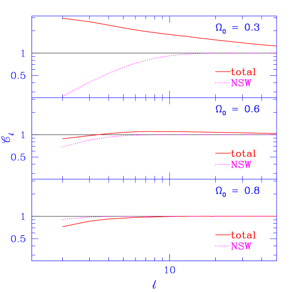
FIG. 1.: The solid curves show the angular power spectrum ${\cal C}_{\ell}$ from the Sachs-Wolfe effect in the three infinite ${\cal H}^{3}$ universes with differing $\Omega_{0}$. Also plotted as a dotted curve is the NSW contribution in each case. The curves are normalized such that the ${\cal C}_{\ell}$ from the NSW contribution goes to unity at large $\ell$. As $\Omega_{0}$ increases towards unity, the relative ISW contribution diminishes and affects smaller values of $\ell$. While the ISW contribution is positive for $\Omega_{0}=0.3$ and $\Omega_{0}=0.6$, it is negative for $\Omega_{0}=0.8$.

Figure 2 illustrates some general features of the distribution of power in $k$-space for the low multipoles of the Sachs-Wolfe CMB anisotropy, using the fourth multipole as an example. While the NSW contribution is always positive, the ISW contribution can be negative due to the interference term. The positive ISW contribution comes from larger values of $k$ than for the NSW effect. Moreover, the small $k$ contribution of the positive NSW effect is countered by the negative interference term in the ISW contribution (the second term in eq. (5)). Note the remarkable cancellation of the NSW contribution for $\Omega_{0}=0.3$. The relative contribution of the ISW effect decreases as $\Omega_{0}\to 1$. The presence of the ISW contribution tends to relax the constraints on the size of a compact universe that can be directly inferred from the suppression of the low multipoles of the CMB anisotropy [16].

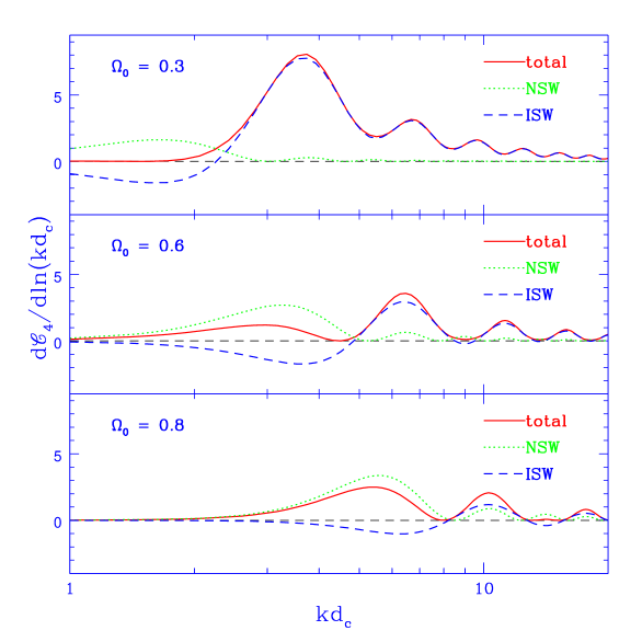
FIG. 2.: The $k$-space dependence of the integrand for the fourth multipole ${\cal C}_{4}$ from the Sachs-Wolfe effect in 3 infinite ${\cal H}^{3}$ universes characterized by the values of $\Omega_{0}$ shown. In each case the dotted and dashed curves are the NSW and ISW contributions, respectively. The ISW curve includes the NSW-ISW interference term as well.

III CMB anisotropy in Compact hyperbolic manifolds

A Brief review of compact spaces

We briefly recapitulate a few basic notions about compact universes that we discussed in paper-I [3]. A compact cosmological model can be constructed by identifying points on the standard infinite flat or hyperbolic FRW spaces by the action of a suitable discrete subgroup of motions, $\Gamma$, of the full isometry group, $G$, of the FRW space. (The isometry group $G$ is the group of motions which preserves the distances between points, i.e., leaves the metric unchanged). The infinite FRW spatial hypersurface is the universal cover, ${\cal M}^{u}$, tiled by copies of the compact space ${\cal M}$. The compact space for a given location of the observer is most appropriately represented as the Dirichlet domain with the observer at its basepoint. Any point ${{\bf x}}$ of the compact space has an image ${{\bf x}}_{i}=\gamma_{i}{{\bf x}}$ in each copy of the Dirichlet domain on the universal cover, where $\gamma_{i}\in\Gamma$. The tiling of the universal cover with Dirichlet domains is a Voronoi tessellation, (a familiar concept in cosmology often used in modeling the large scale structure in the universe), with the seeds being the basepoint and its images. By construction a Dirichlet domain represents the compact space as a convex polyhedron with even number of faces identified pairwise under $\Gamma$. In cosmology, the Dirichlet domain constructed around the observer represents the universe as ‘seen’ by the observer and it proves useful in this context to define the outradius, $R_{>}$, the radii of the circumscribing sphere (smallest sphere around the observer which encloses the Dirichlet domain) and, the inradius, $R_{<}$, the radii of the inscribed sphere (largest sphere around the observer which can be enclosed within the Dirichlet domain) of the Dirichlet domain [5]. Note that $R_{>}$ and $R_{<}$ are specific to the location of the observer within the compact space since the Dirichlet domains around different observers are not necessarily identical. An observer-independent (and Dirichlet-domain-independent) linear measure of the size of the compact space is given by the diameter of the space, $d_{\!\cal M}\equiv\sup_{x,y\in{\cal M}}d(x,y)$ [17, 18], i.e., the maximum separation between two points in the compact space.

For cosmological CH models, ${\cal M}^{u}\equiv{\cal H}^{3}$, the three-dimensional hyperbolic (uniform negative curvature) manifold. ${\cal H}^{3}$ can be viewed as a hyperbolic section embedded in four dimensional flat Lorentzian space. The isometry group of ${\cal H}^{3}$ is the group of rotations in the four space – the proper Lorentz group, $SO(3,1)$. A CH manifold is then completely described by a discrete subgroup, $\Gamma$, of the proper Lorentz group, $SO(3,1)$. The Geometry Centre at the University of Minnesota has a large census of CH manifolds and public domain software SnapPea [19]. We have adapted this software to tile ${\cal H}^{3}$ under a given topology using a set of generators of $\Gamma$. The tiling routine uses the generator product method and ensures that all distinct tiles within a specified tiling radius are obtained.

A CH manifold, ${\cal M}$, is characterized by a dimensionless number, ${\cal V}_{\!\cal M}\equiv V_{\!\cal M}/d_{c}^{3}$, where $V_{\!\cal M}$ is the volume of the space and $d_{c}$ is the curvature radius [20]. There are a countably infinite number of CH manifolds with no upper bound on ${\cal V}_{\!\cal M}$. The theoretical lower bound stands at ${\cal V}_{\!\cal M}\geq 0.167$ [21]. The smallest CH manifold discovered so far has ${\cal V}_{\!\cal M}=0.94$ [22]. The Minnesota census lists several thousands of these manifolds with ${\cal V}_{\!\cal M}$ up to $\sim 7$. In the cosmological context, the physical size of the curvature radius $d_{c}$ is determined by the density parameter and the Hubble constant $H_{0}$: $d_{c}=(c/H_{0})/\sqrt{1-\Omega_{0}}$. The physical volume of the CH manifold with a given topology, i.e., a fixed value of $V_{\!\cal M}/d_{c}^{3}$, is smaller for smaller values of $\Omega_{0}$.

B Computing spatial correlation functions

Here we summarize the main result of our regularized method of images that is discussed in detail in paper-I [3]. The correlation function on a compact space (and more generally, any non-simply connected space), ${\cal M}={\cal M}^{u}/\Gamma$, can be expressed as a regularized sum over the correlation function on its universal cover, ${\cal M}^{u}$, calculated between ${\bf x}$ and the images $\gamma{\bf x^{\prime}}$ ($\gamma\in\Gamma$) of ${\bf x^{\prime}}$:

$$\xi^{c}_{\Phi}({\bf x},{\bf x}^{\prime}) = \widetilde{\sum_{\gamma\in\Gamma}}\xi^{u}_{\Phi}({\bf x},\gamma{\bf x}^{\prime})$$ (7)

$$= \sum_{\gamma\in\Gamma}\xi^{u}_{\Phi}({\bf x},\gamma{\bf x}^{\prime})-\frac{1}{V_{\!\cal M}}\int_{{\cal M}^{u}}d{\bf x^{\prime}}~{}\xi^{u}_{\Phi}({\bf x},{\bf x}^{\prime})\,.$$ (8)

The local isotropy and homogeneity of ${\cal H}^{3}$ implies $\xi^{u}_{\Phi}({\bf x},{\bf x}^{\prime})$ depends only on the proper distance, $r\equiv d({\bf x},{\bf x^{\prime}})$, between the points ${\bf x}$ and ${\bf x^{\prime}}$. The eigenfunctions on the universal cover are of course well known for all homogeneous and isotropic models [23]. Consequently $\xi^{u}_{\Phi}({\bf x},{\bf x}^{\prime})$ can be obtained using its eigenmode expansion. The initial power spectrum $P_{\Phi}(k)$ is believed to be dictated by an early universe scenario for the generation of primordial perturbations. We assume that the initial perturbations are generated by quantum vacuum fluctuations during inflation. This leads to

$$\xi^{u}_{\Phi}({\bf x},{\bf x}^{\prime})\equiv\xi^{u}_{\Phi}(r)=\int_{0}^{\infty}\frac{d\beta~{}\beta}{(\beta^{2}+1)}~{}\frac{\sin(\beta r)}{\beta\sinh r}~{}~{}{\cal P}_{\Phi}(\beta)\,,$$ (9)

where $\beta\equiv\sqrt{(kd_{c})^{2}-1}$ and ${\cal P}_{\Phi}(\beta)\equiv\beta(\beta^{2}+1)P_{\Phi}(k)/(2\pi^{2})$.

In the simplest inflationary models, ${\cal P}_{\Phi}$, the power per logarithmic interval of $k$ is approximately constant in the subcurvature sector, defined by $kd_{c}>1$. This is the generalization of the Harrison-Zeldovich spectrum in spatially flat models to hyperbolic spaces [24, 25]. Sub-horizon vacuum fluctuations during inflation are not expected to generate supercurvature modes, those with $kd_{c}<1$, which is why they are not included in eq.(9). Indeed, since $H^{2}>1/(ad_{c})^{2}$, for modes with $kd_{c}<1$ we always have $k/(aH)<1$ so inflation by itself does not provide a causal mechanism for their excitation. Moreover, the lowest non-zero eigenvalue in compact spaces, $k_{1}>0$, provides an infra-red cutoff in the spectrum which can be large enough in many CH spaces to exclude the supercurvature sector entirely ($k_{1}d_{c}>1$). (See  [3].) Even if the space does support supercurvature modes, some physical mechanism needs to be invoked to excite them, e.g., as a byproduct of the creation of the compact space itself, but which could be accompanied by complex nonperturbative structure as well. To have quantitative predictions for $P_{\Phi}(k)$ would require addressing this possibility in a full quantum cosmological context. We note that our main conclusions regarding peculiar correlation features in the CMB anisotropy (see $\S$ IV) would qualitatively hold even in the presence of supercurvature modes.

Although equation (8) encodes the basic formula for calculating the correlation function, it is not numerically implementable as is. Both the sum and the integral in equation (8) are divergent and the difference needs to be taken as a limiting process of summation of images and integration up to a finite distance $r_{*}$:

$$\xi^{c}_{\Phi}({\bf x},{\bf x}^{\prime})=\lim_{r_{*}\to\infty}\left[\sum_{r_{j}<r_{*}}\xi^{u}_{\Phi}(r_{j})-\frac{4\pi}{V_{\!\cal M}}\int_{0}^{r_{*}}dr~{}\sinh^{2}r~{}\xi^{u}_{\Phi}(r)\right],~{}~{}~{}~{}r_{j}=d({\bf x},\gamma_{j}{\bf x}^{\prime})\,.$$ (10)

The volume element in the integral is the one appropriate for ${\cal H}^{3}$. Numerically we have found it suffices to evaluate the above expression up to $r_{*}$ about $4$ to $5$ times the domain size $R_{>}$ to obtain a convergent result for $\xi^{c}_{\Phi}({\bf x},{\bf x}^{\prime})$.

C Computing the CMB correlation

For Gaussian perturbations, the angular correlation function, $C(\hat{q},\hat{q}^{\prime})$, completely encodes the CMB anisotropy predictions of a model. To make maps, the celestial sphere is discretized into $N_{p}$ pixels labeled by $p$. $N_{p}$ is determined by the angular resolution, $\sim 7^{\circ}$ degrees for cobe–dmr . The cobe–dmr maps had $(2.6^{\circ})^{2}$ pixels, corresponding to $N_{p}=6144$, though compressing the data into $N_{p}=1536$ pixels leads to no information loss. We use this number of pixels in § V, where we confront our models with the cobe–dmr observations using Bayesian statistical methods, and also in the maps shown in this paper.

For Gaussian statistics, the pixelized theoretical maps are fully determined by the $N_{p}\times N_{p}$ pixel-pixel correlation matrix, $C_{Tpp^{\prime}}\equiv C(\hat{q}_{p},\hat{q}_{p^{\prime}})$. The expression for $C(\hat{q},\hat{q}^{\prime})$ in eq. (5) involves an integral along the line of sight from the observer to the surface of last scattering – the integrated Sachs–Wolfe term (ISW). We find that a simple integration rule using $N_{L}$ points along each line of sight gives accurate results when the points are spaced at equal increments $\Delta F$ of $F(\tau)$. Consequently, to get the full $C_{Tpp^{\prime}}$ matrix we need to evaluate the correlation function, $\xi^{c}_{\Phi}({\bf x},{\bf x}^{\prime})$, between $N_{p}(N_{p}+1)N_{L}^{2}/2$ pairs of points on the constant-time hypersurface of last scattering:

$$C_{Tpp^{\prime}}=\frac{1}{9}\xi^{c}_{\Phi}({\chi_{\!{}_{\rm H}}}\hat{q}_{p},{\chi_{\!{}_{\rm H}}}\hat{q}_{p^{\prime}})+\frac{2}{3}~{}\frac{\Delta F}{N_{L}}\sum_{i=1}^{N_{L}}w_{i}\left[\xi^{c}_{\Phi}({\chi_{\!{}_{\rm H}}}\hat{q}_{p},\chi_{i}\hat{q}_{p^{\prime}})+\xi^{c}_{\Phi}(\chi_{i}\hat{q}_{p^{\prime}},{\chi_{\!{}_{\rm H}}}\hat{q}_{p})\right]+4~{}\left(\frac{\Delta F}{N_{L}}\right)^{2}\sum_{i=1}^{N_{L}}\sum_{j=1}^{N_{L}}w_{ij}\xi^{c}_{\Phi}(\chi_{i}\hat{q}_{p^{\prime}},\chi_{j}\hat{q}_{p})$$ (11)

where $w_{i}$ and $w_{ij}$ are ${\cal O}(1)$ coefficients that depend on the specific difference scheme used.

To calculate $C_{Tpp^{\prime}}$ in the standard infinite open cosmological models with this real-space integration to an accuracy comparable to that of the traditional evaluation in $k$–space, $N_{L}\sim 10$ is sufficient. Moreover, the real space integration is much faster in terms of CPU time. For the method to remain accurate in compact models, $N_{L}$ should, of course, exceed the number of the times a typical photon path crosses the compact Universe. We found $N_{L}\sim 10$ is still enough for the models we have analyzed so far.

IV Correlation features in the CMB anisotropy

In standard cosmological models based on a topologically trivial space such as ${\cal H}^{3}$, the observed CMB photons have propagated along radial geodesics from a $2$-sphere of radius $R_{\sc ls}$ (that we refer to as the sphere of last scattering, SLS) centered on the observer. The same picture also applies to CH models when the space is viewed as a tessellation of the universal cover tiled by the Dirichlet domain with the observer at the basepoint. If $V_{\sc LS}$, the volume of the SLS, is much larger that that of the compact space, the photons propagate through a lattice of identical domains. As a consequence, strong correlations build up between CMB temperature fluctuations observed in widely separated directions. The correlation function $C(\hat{q},\hat{q}^{\prime})$ is anisotropic and contains characteristic patterns determined by the photon geodesic structure of the compact manifold. These correlations persist even in CH models whose Dirichlet domains are comparable to or slightly bigger than the SLS. This is the key difference from the standard models where $C(\hat{q},\hat{q}^{\prime})$ depends only on the angle between $\hat{q}$ and $\hat{q}^{\prime}$ and generally falls off with angular separation.

The pattern of strong correlations is directly linked to the way the points (on the universal cover ${\cal M}^{u}$) enclosed by the SLS are equivalent under the topological identification $\Gamma$. Consider a set of points $S$ on the universal cover. Then for all $\gamma\in\Gamma$ the pair of subsets $\gamma S\cap S$ and $S\cap\gamma^{-1}S$ are equivalent under $\Gamma$, i.e., either contain the same points of the compact space ${\cal M}$ or they are both empty. (Obviously, the isometry $\gamma^{-1}\in\Gamma$ maps the first set onto the second.) If $S$ consists of the points on the SLS, a non-empty set $S\cap\gamma S$ would be a circle on the SLS which is pointwise identical to another circle $S\cap\gamma^{-1}S$ on the SLS. If the CMB anisotropy is dominated by the surface term, then the CMB temperature along one circle is expected to be identical to that along the other circle. This effect was first understood and much emphasized in the works byCornish, Starkman and Spergel [28]. The necessary and sufficient condition for the existence of matched circles (non empty subsets $S\cap\gamma S$) on the SLS is that $R_{\sc ls}\geq R_{<}$, i.e., the SLS is not completely enclosed within the Dirichlet domain. We discuss the CMB correlations in our models that arise from this kind of identification in $\S$ IV A.

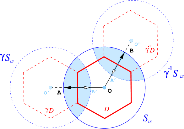
FIG. 3.: The origin of CMB correlation patterns in a multiply connected universe is illustrated. The compact space is represented by the (hexagonal) Dirichlet domain, $D$, around the observer, $O$, which tiles the universal cover. The tiles $\gamma D$ and $\gamma^{-1}D$ under one of the face translations $\gamma\in\Gamma$ and its inverse are shown. The points $O^{\prime}$ and $O^{\prime\prime}$ are the images of the observer, $O$, under $\gamma$ and $\gamma^{-1}$, respectively. The point $B^{\prime}$ is the $\gamma$-translate of $B$ and the point $A^{\prime}$ is the $\gamma^{-1}$ translate of $B$. The solid circle $S_{LS}$ represents the sphere of last scattering (SLS) on the universal cover; the dashed circles, labeled $\gamma S_{LS}$ and $\gamma^{-1}S_{LS}$, are the translates of SLS under $\gamma$ and $\gamma^{-1}$ , respectively. The intersections of the sphere $S_{LS}$ with $\gamma S_{LS}$ and $\gamma^{-1}S_{LS}$ create a matched pair of circles on the SLS. Similarly, the shaded lens-shaped regions within the $SLS$ consist of identical sets of points. Consider the lines of sight $OA$ and $OB$ directed towards the centers of the matched circles. The ray $O^{\prime}B^{\prime}$ is the image of $OB$ under $\gamma$ and the ray $O^{\prime\prime}A^{\prime}$ is the image of $OA$ under $\gamma^{-1}$. By the arguments outlined in the text, the segment $AB^{\prime}=OA\cap OB^{\prime}$ is identical to $A^{\prime}B=OB\cap OA^{\prime}$.

The CMB anisotropy has contributions from the entire line of sight and it is useful to study the subsets of identical points enclosed by the SLS. If $S$ is the set of all points enclosed by the SLS, then the pairs of subsets of $S$ that are identical are lens-shaped regions created by the intersection of two balls (See Figure 3). Again the necessary and sufficient condition for the existence of such identified regions within the SLS is $R_{\sc ls}\geq R_{<}$. Further if the SLS does not enclose more than one Dirichlet domain, these lens-like regions are in the direction of the faces and are adjacent to the SLS. (We find from our analysis of the cobe–dmr constraints that viable CH models have volumes comparable to or more than that enclosed within the SLS. See $\S$ V.) In these cases it is clear that correlation patterns are built from points close to the SLS and directly reflect the shape of polyhedral Dirichlet domain.

The ISW-CMB correlation depends on the correlations between the points lying on the two (radial) lines of sight from the observer to the SLS. Hence it is instructive to study whether two different lines of sight (radial lines) in the SLS contain a set of identical points. Consider the set of points $L_{1}$ and $L_{2}$ along two distinct lines of sight. Then for all $\gamma\in\Gamma$, the subset $L_{1}\cap\gamma^{-1}L_{2}$ of $L_{1}$, if non-empty, would contain the same points as the subset $\gamma L_{1}\cap L_{2}$ of $L_{2}$. The necessary and sufficient condition for the existence of such pairs of lines of sight is again $R_{\sc ls}\geq R_{<}$. It is possible to show that there are infinite pairs of lines of sights which share at least one common point, but what is more interesting and relevant are the pairs where the identical subsets contain a segment. It is a straightforward exercise to verify that every pair of lines of sight pointing towards centers of matched circles discussed above must contain a segment consisting of identical points (See Figure 3). As we shall discuss in $\S$ IV B, this result is important in understanding the correlation patterns in CMB anisotropy when the integrated Sachs Wolfe contribution is significant.

In the regime where $R_{\sc ls}<R_{<}$, there are no points within the SLS that are topologically equivalent and the specific correlation features discussed above are absent. However, quantitatively the CMB correlations continue to have observable deviations from that expected in a simply connected model until $R_{\sc ls}$ is substantially smaller than $R_{<}$. Typically, the correlation pattern around any point in the sky is anisotropic and distorted.

In simply connected models of the universe, the global homogeneity and isotropy ensures that the CMB sky is statistically equivalent for all observers. These global symmetries are generically absent in compact (open or flat) universe models. Consider two distinct observers. If one of them measures the correlation function between pairs $({\bf x},{\bf x}^{\prime}$), the corresponding measurement for the other one will be between pairs $(g{\bf x},g{\bf x}^{\prime})$ where $g$ is the element of the isometry group of the universal cover, $g\in G^{u}$, which transports the first observer to the position of the second one. (The motion $g$ always exists since the universal cover is homogeneous.) For example if ${\bf x},{\bf x}^{\prime}$ belong to the SLS as seen by first observer, then $g{\bf x},g{\bf x}^{\prime}$ are on the SLS from the second observer’s point of view. Each pairwise correlation value $\xi^{c}_{\Phi}({\bf x},{\bf x}^{\prime})$ is determined by the set of distances ${\cal D({\bf x},{\bf x}^{\prime})}=\{d({\bf x},\gamma_{j}{\bf x}^{\prime})$, $\gamma_{j}\in\Gamma\}$. Moving the observer translates this set to $\{d(g{\bf x},\gamma_{j}g{\bf x}\prime)\}$. Since $G^{u}$ is the isometry group on the universal cover, it conserves distances; in particular, $d(g{\bf x},\gamma_{j}g{\bf x}\prime)=d(g^{-1}g{\bf x},g^{-1}\gamma_{j}g{\bf x}\prime)$. Thus, under a general relocation of the observer by $g$, the set of distances ${\cal D({\bf x},{\bf x}\prime)}$ is transformed as $\{d({\bf x},\gamma_{j}{\bf x}\prime)\}\rightarrow\{d({\bf x},g^{-1}\gamma_{j}g{\bf x}\prime)\}$.

If $\Gamma$ is a normal/invariant subgroup of $G^{u}$, ($g^{-1}\gamma g\in\Gamma,\forall\gamma\in\Gamma,g\in G^{u}$), moving the observer simply reshuffles the terms in the set ${\cal D}$, and $\xi^{c}_{\Phi}({\bf x},{\bf x}^{\prime})$=$\xi_{\Phi}^{c}(g{\bf x},g{\bf x}^{\prime})$. This is the case with simple tori, in which opposite sides are identified by pure translation without rotation. In the case of CH spaces (as well as tori with twists), $\Gamma$ is not a normal subgroup of $G^{u}$. Equivalent only are those observers mapped by a $g$ belonging to the isometry group $G$ of the compact space ${\cal M}$ itself, not in the larger isometry group of its cover ${\cal M}^{u}$. Each element of the isometry group $G$ on ${\cal M}$ commutes with all the elements of $\Gamma$, with the immediate result that the $C_{Tpp^{\prime}}$ calculated will be the same up to rotations of the sky if the observer is moved along the orbits of $G$ in ${\cal M}$.

In $\S$ IV C, we discuss the correlation pattern in the CMB that arises due to the global inhomogeneity of the compact space.

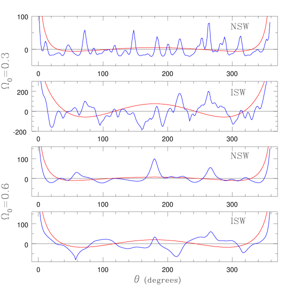
FIG. 4.: This shows the behavior of the correlation function of the CMB temperature on a great circle in the sky in a CH model (m004(-5,1)). The solid curves in the first and third panels show $C(\theta)$ for the surface term in the Sachs-Wolfe effect (NSW) for $\Omega_{0}=0.3$ and $0.6$, respectively. They reflect the spatial correlation along a circle on the sphere of last scattering (SLS). The number of peaks in $C(\theta)$ matches the number of Dirichlet domains that the circle intersects. The smooth curves show corresponding results for the simply connected infinite ${\cal H}^{3}$ models with $\Omega_{0}=0.3$ and $0.6$. The second and fourth panels are analogous to the first and third panels, except with the integrated Sachs-Wolfe (ISW) effect included. In this more physically correct case, the sharp NSW peaks have been diluted by the ISW contributions. However, the ISW effect induces new features; in particular, note the appearance of strong negative correlations in panels two and four.

A Correlations due to the NSW Surface term alone

In Figure 4 the complex behavior of the correlation function is illustrated with the example of the small CH model (m004(-5,1)). The SLS encompasses $\approx 150$ domains for $\Omega_{0}=0.3$ and $\approx 20$ domains for $\Omega_{0}=0.6$. It is comparable to the size of one domain for $\Omega_{0}=0.9$. The angular correlation along any arbitrary great circle in the sky in lower $\Omega_{0}$ models shows distinct peaks as one encounters repeated copies of the Dirichlet domain. The peaks are more pronounced when one considers only the surface terms of eq.(2) in the CMB anisotropy. Including the line of sight ISW contribution tends to smearing the peaks, but also adds its own characteristic features as discussed in $\S$ IV B.

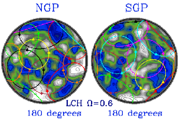
FIG. 5.: This shows two full-sky (noiseless) CMB anisotropy maps, plotted as pairs of $180^{\circ}$ diameter hemispherical caps, one centered on the South Galactic Pole (SGP) and one on the North (NGP). They are one of an infinite number of possible random realizations based on the computed pixel-pixel correlation matrix for the model in question. Both surface and integrated Sachs-Wolfe effects have been included. The power was normalized to best match the cobe–dmr data. The contours are linearly spaced in $30~{}\mu{\rm K}$ steps. In contrast to Figs. 10 and 11, the maps are not optimally filtered. The model labels $L(arge)CH$ and $S(mall)CH$ refer to the CH models v3543(2,3) and m004(-5,1), respectively. (The model number associated with the topology corresponds to that of the census of CH spaces from the Geometry center, Univ. of Minnesota; $SCH$ is one of the smallest and $LCH$ is one of the largest spaces in the census.) The value of $\Omega_{0}$ in each was chosen so that $V_{\!\cal M}\sim V_{\sc sls}$. The matched pairs of circles expected if the CMB anisotropy is dominated by the surface terms [28] are superimposed on the map for each model. Each pair is labeled by the same number centered on the circles. The relative phase is shown by identified points marked by a diamond and a triangle on each circle in a pair. For clarity, we show only the eight largest pairs out of $35$ for the $LCH_{\Omega_{0}=0.6}$ case. Even at cobe–dmr resolution, we find the cross-correlation between the temperature along matched circles is very good in the $SCH_{\Omega_{0}=0.9}$ model. The ISW contribution is larger at $\Omega_{0}=0.6$, and the cross-correlation coefficients are systematically smaller for $LCH_{\Omega_{0}=0.6}$ circle pairs.

Consider compact universe models which are small enough such that the SLS does not completely fit inside one domain, $R_{\sc ls}>R_{<}$. The CMB temperature is expected to be identical along pairs of circles if temperature fluctuations are dominated by the surface terms at the SLS [28]. We identify these matched circles on the sky in our models and check the extent of cross correlation seen at the angular resolution of cobe–dmr . Figure 5 shows the matched pairs of circles in two (“small” and “large”) CH models superimposed on random realizations of the theoretical sky generated from the appropriate pixel-pixel correlation matrices. The models were chosen to have a volume comparable to the volume $V_{\sc LS}$ within the SLS. Even with the coarse pixelization of cobe–dmr, we do see fairly good cross-correlation in the CMB temperature along matched circles in our realizations. Again, the pattern of correlated circles is more pronounced when the Sachs-Wolfe surface term is dominant, as happens in the small model ($SCH$) with $\Omega_{0}=0.9$. We compute the cross-correlation coefficient between the temperature fluctuations along two matched circles $C_{1}$ and $C_{2}=\gamma C_{1}$,

$$\rho_{12}=\langle\Delta T({\bf x})\Delta T(\gamma{\bf x})\rangle/\left[\langle\Delta T({\bf x})^{2}\rangle\langle\Delta T(\gamma{\bf x})^{2}\rangle\right]^{1/2},~{}{\bf x}\in C_{1},~{}\gamma{\bf x}\in C_{2}\,.$$ (12)

(In the case of a single realization we replace the statistical average by the integration over ${\bf x}$ along the circles.) In the $SCH$ $\Omega_{0}=0.9$ case, $\rho_{12}$ is in the range $0.6-0.95$, whereas it is in the range $0.2-0.6$ for the large model ($LCH$) with $\Omega_{0}=0.6$.

The circles of identified pixels on the SLS are not the whole story. Enhanced NSW cross-correlations, but at a lower level, also exist between all pairs of points on the SLS which are projected close to each other on the CH manifold. This can be seen as secondary maxima in the examples in Figure 4; these are absent in standard cosmological models. Some features persist at a detectable level even when the compact universe encompasses the SLS, i.e., $R_{\sc ls}\mathrel{\hbox to0.0pt{\lower 3.0pt\hbox{$\mathchar 536\relax$}\hss}\raise 2.0pt\hbox{$\mathchar 316\relax$}}R_{<}$ , although circles are absent in this case (the effect dies out for $R_{\sc ls}\ll R_{<}$). When the relative ISW component is significant, the geometrical patterns based on pointwise identifications on the SLS are supplanted by more complex features arising from identifications between photon geodesics, e.g., the strong negative correlations evident in Figure 4.

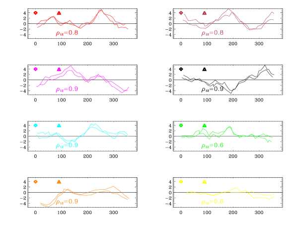
FIG. 6.: In the eight panels of the figure, the CMB temperature along the $8$ matched pairs of circles of the SCH model shown in Figure 5 (top panel) is plotted as a function of a polar angle. The temperature shown is from the same realization of the CMB sky that is used in Figure 5 and the diamond and triangles are in correspondence. The CMB anisotropy includes both the surface and integrated Sachs-Wolfe effects. At $\Omega_{0}=0.9$, the ISW contribution is small, and thus the values of the correlation coefficient are high.

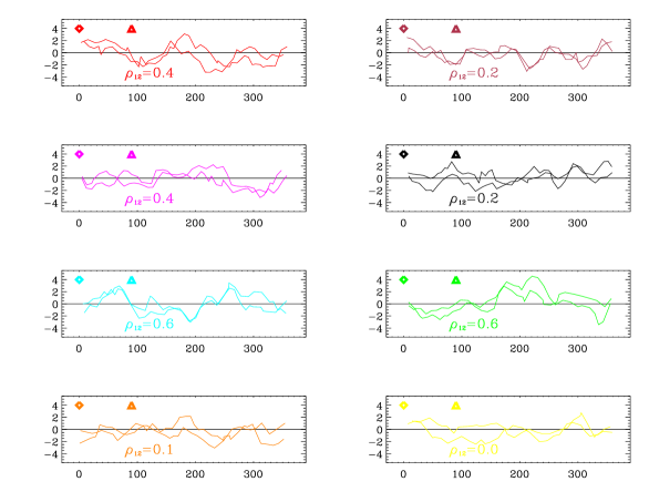
FIG. 7.: In the eight panels of the figure, the CMB temperature along the largest $8$ matched pairs of circles of the LCH model ($\Omega_{0}=0.6$) shown in Figure 5 (bottom panel) is plotted as a function of a polar angle. The temperature shown is from the same realization of the CMB sky that is used in Figure 5 and the diamond and triangles markers are in correspondence. The CMB anisotropy includes both the surface and integrated Sachs-Wolfe effects. At $\Omega_{0}=0.6$, the ISW contribution is significant, resulting in small values of the correlation coefficient.

B Correlations with the ISW effect included

In a hyperbolic model, the temperature fluctuations depends on the entire path of the photons from the sphere of last scattering to the observer. The relative contribution of the ISW effect increases as the value $\Omega_{0}$ decreases. As the ISW component increases, it tends to wash out the patterns arising solely from the NSW (described in the previous section). However, it also introduces additional features in the CMB correlation. In Figures 6 and  7, the temperature fluctuations along matched pairs of circles in a realization are plotted. Since $\Omega_{0}$ is closer to unity in the small model ($SCH$), the temperature fluctuations along the circles are more tightly correlated than in the large model ($LCH$).

An example of ISW-induced features is the significant negative correlations between widely separated directions in the sky, as is clearly seen in the panels two and four of Figure 4. In fact, the highly anti-correlated regions tend to lie at the centers of the matched circles discussed in $\S$ IV A. Figure  8 plots the anticorrelated pairs of pixels separated by more that $\approx 10^{\circ}$ below a threshold in the correlation coefficient of $C_{pp\prime}/\sqrt{C_{pp}C_{p\prime p\prime}}=-0.3$ in the LCH model with $\Omega_{0}=0.6$. This should be contrasted with the highest levels of anticorrelation of $\approx-0.04$ predicted in the corresponding simply connected universe.

As discussed earlier, the lines of sight pointing to centers of matched circles have segments of identical points and this can lead to anticorrelation between the CMB anisotropy in those directions. Here we explain this with the help of Figure 3. The segments $AB^{\prime}$ and $A^{\prime}B$ of lines of sight $OA$ and $OB$ are identical under $\Gamma$. (Recall eqs.(5) and (11) for the Sachs-Wolfe contribution to the correlation between temperature fluctuations in two directions in the sky.) The surface term depends on the correlation of the potential, $\Phi$, between two points physically separated by the distance $r_{1}$. The interference term however contains correlation between identical points, $AA^{\prime}$ and $BB^{\prime}$, and close ones. The integral term has correlations between close points but is down-weighted by the extra factor of $\Delta F$. Thus the interference term (which is usually small in simply connected models) in this particular setting can dominate the total CMB correlation and make it negative. Thus the existence of strongly anticorrelated spots caused by the ISW term is a signature of non-trivial topology.

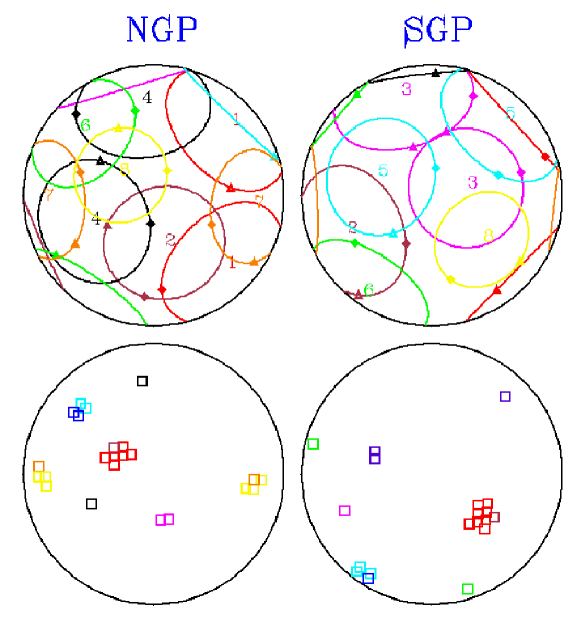
FIG. 8.: The negative correlation between pixels located at the center of matched circles is demonstrated. The top panel shows the $8$ largest circle pairs for the LCH model on a sky map, as in Figure 5. The groups of pixels marked out in the lower sky map are distant pairs with high anticorrelation, $C_{pp\prime}/\sqrt{C_{pp}C_{p\prime p\prime}}<-0.3$. It is visually apparent that these regions lie at the centers of matched circles and are labeled accordingly.

C Patterns Arising from Global Inhomogeneity

The global inhomogeneity of compact spaces implies that the variance of the the gravitational potential is spatially dependent. If these fluctuations arose from quantum noise during inflation, $\Phi({\bf x})$ would be an inhomogeneous Gaussian random field, with a pattern of inhomogeneity determined by the topology of the compact space.

The CH models that we have considered also predict that the rms temperature fluctuations in the sky vary with direction, as is shown in Fig. 9 and in Fig. 10 of Paper 1. In both LCH and SCH models there are ‘loud’ spots – directions in the sky where the variance is significantly larger. For the NSW contribution, these arise when the SLS crosses loud regions in the Dirichlet domain where the variance $\xi^{c}_{\Phi}({\bf x},{\bf x})$ is large. These regions consist of points in the Dirichlet domain where the length of the shortest geodesic is small compared to the typical size of the shortest closed geodesic at other points, i.e., the closest image of the point on the universal cover is smaller than $\sim R_{<}$. The LCH model has a loud region around a vertex of the Dirichlet domain shared by two pairs of identified faces where the nearest image of the points close to this vertex are at a small separation. We discussed this effect and results for the NSW effect in a previous paper [3]. Fig. 9 shows the extent to which the ISW term masks the signature expected from a simple NSW consideration: the loud spot is dramatically modified, even changing sign, when ISW is included.

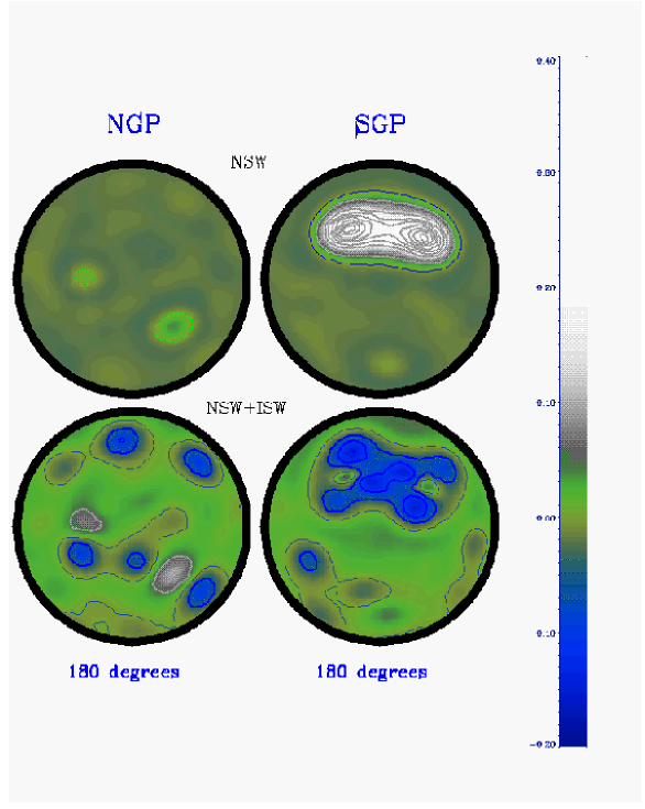
FIG. 9.: The figure shows two full-sky maps of the fluctuations in the standard deviation of the predicted CMB temperature, plotted as pairs of $180^{\circ}$ diameter hemispherical caps, one centered on the South Galactic Pole (SGP) and one on the North (NGP). The contours are linearly spaced in units of 0.03 of the mean standard deviation. The first map considers only the NSW contribution, where at the peak value standard deviation is 45% larger than its mean value . The second plot shows that the significant ISW contribution at $\Omega_{0}=0.6$ radically alters the pattern of fluctuations in the variance since the CMB temperature now depends on the potential along the entire line of sight.

There are known examples of multiply connected spaces where the pattern of inhomogeneity is a dominant observable effect. In [29] a non-compact but multiply connected horn topology was constructed and the properties of the perturbations were studied. It was demonstrated that there is a region in which the variance of $\Phi$ is strongly suppressed and would correspond to a dark spot in the distribution of galaxies. For the NSW contribution to the CMB anisotropy, this same effect directly translates to suppression of the variance of the temperature fluctuations in the corresponding direction, creating a flat spot signature in the CMB anisotropy, shown explicitly for the toroidal horn space in [30].

V Bayesian analysis constraints from COBE-DMR

In this section, the goal is to explicitly evaluate how likely the various compact universe models are in light of the COBE data on angular anisotropies. We first review the statistical distributions for the maps derived from the COBE data, then show how we use our techniques to confront the data.

The raw data of a CMB experiment comes in the form of a time stream of measurements $d_{t}$ at $N_{t}$ time-ordered points for each frequency channel. The data are then binned into a $N_{p}$-pixel discretization of the sky, through the relation $d_{t}=\sum_{p}P_{tp}\Delta_{p}+\eta_{t}$, where the $N_{t}\times N_{p}$ pointing matrix $P_{tp}$ maps the observing time to the angular position at that time and $\eta_{t}$ is the time stream noise. $\Delta_{p}$ is the true signal on the sky. With the (reasonable and checkable) assumption that the noise is Gaussian with covariance matrix $N=\langle\eta_{t}\eta_{t^{\prime}}\rangle$, one can find the map $\bar{\Delta}$ which maximizes the conditional probability ${\cal P}(d|\Delta)$ and the pixel-pixel noise covariance matrix about it, $C_{N}$.

$$\bar{\Delta}=C_{N}P^{\dagger}N^{-1}d\,,~{}~{}~{}~{}~{}C_{N}=(P^{\dagger}N^{-1}P)^{-1}\,,$$ (13)

No larger moments required, given the Gaussian noise assumption. Thus, the probability of the data given the true sky signal $\Delta$ is

$${\cal P}(\bar{\Delta}|\Delta)=\frac{1}{(2\pi)^{N_{p}/2}\|C_{N}\|^{1/2}}e^{-\frac{1}{2}(\Delta-\bar{\Delta})^{\dagger}C_{N}^{-1}(\Delta-\bar{\Delta})}\,,$$ (14)

where $C_{N}=\langle(\Delta-\bar{\Delta})(\Delta-\bar{\Delta})^{\dagger}\rangle$. Provided the pixelization is fine-grained enough, the $\bar{\Delta}$ map plus the $C_{N}$ contain all of the sky information present in the original data set $d_{t}$.

The COBE team[26] have given 6 maps at 3 frequencies, 31, 53, and 90 GHz, each of 6144 pixels of size $(2.6^{o})^{2}$, along with information to construct $C_{N}$ from the number of observations made in each pixel and the average noise in the radiometers over an observing time. Four our analysis, we compressed the six cobe–dmr maps [26] into a (A+B)(31+53+90 GHz) weighted-sum map. Galactic emission near the plane of the Galaxy sufficiently contaminates the primordial signal that a region $\pm 20^{\circ}$ from the Galactic plane is removed, along with adjacent extra pixels in which contaminating Galactic emission is known to be high, as advocated by the DMR team. Although one can do analysis with the map’s $(2.6^{\circ})^{2}$ pixels, this “resolution 6” pixelization of the quadrilateralized sphere is oversampled relative to the cobe–dmr beam size, and there is no effective loss of information if we do further data compression by using “resolution 5” pixels, $(5.2^{\circ})^{2}$ [27]. The celestial sphere is then represented by $N_{p}=1536$ pixels before the Galactic cut, with $N_{p}=999$ pixels remaining after the cut is made. Our $C_{N}$ is largely diagonal, but we include the off-diagonal components centered on a $60^{\circ}$ pixel-pair angle separation, which corresponds to the horn separation of the instrument. We remove a best-fit monopole and dipole from the cut-sky maps. Proper account is taken of the monopole and dipole contributions, as well as possible quadrupole contamination by Galaxy emission, by increasing the noise in associated template patterns [31, 32]. This corresponds to having arbitrary monopole, dipole and quadrupole contamination possible, and effectively “shorts-out” this contributions to $C_{T}$.

Now we need a probabilistic model for the signal. There may be several physically different signals in the cobe–dmr data - not only primordial CMB anisotropy, but also Galactic emission and others. However, except for the quadrupole contamination which we corrected for, the contribution of signals other than CMB is small in the weighted sum (over frequency channels) maps that we have used. We have assumed a Gaussian probability distribution for the primordial fluctuations of $\Phi$. As we have seen $\Delta T/T$ is linearly related to $\Phi$, which remains true even if all the effects leading to the CMB anisotropy are included. Thus, $\Delta T/T$ is also statistically a Gaussian random field, fully described by the theoretical pixel-pixel correlation matrix $C_{T}$ that we have focused on in our computations:

$${\cal P}(\Delta|C_{T})=\frac{1}{(2\pi)^{N_{p}/2}\|C_{T}\|^{1/2}}e^{-\frac{1}{2}\Delta^{\dagger}C_{T}^{-1}\Delta}\,,~{}~{}~{}~{}~{}~{}C_{T}=C(\hat{q}_{p},\hat{q}_{p^{\prime}})\,.$$ (15)

The $C_{T}$ which enters here should have the COBE beam taken into account. We do this by calculating $C_{T}$ through eq.(11). We used a high $k$-cutoff in evaluating the $C^{u}$, choosing its value to regulate the high frequency part of $C_{T}$, but ensured that it was much higher than the corresponding scale associated with the COBE beam size. The effect of the COBE beam was included by forming $B^{\dagger}C_{T}B$, where $B_{pp^{\prime}}$ is the COBE beam between pixels $p$ and $p^{\prime}$, related to the beam-shape $B_{\ell}$ by

$$B_{pp^{\prime}}=\sum_{\ell}{(2\ell+1)\over 4\pi}B_{\ell}P_{\ell}(\hat{q}_{p}\cdot\hat{q}_{p^{\prime}})\,.$$ (16)

This gives all the necessary ingredients for our analysis except for a prior probability ${\cal P}(C_{T})$ for the theory, which may encode both our theoretical prejudices about the models and results from other observational tests. For the moment we leave ${\cal P}(C_{T})$ unspecified and concentrate on the likelihood function of a model

$${\cal L}(C_{T})\equiv{\cal P}(\bar{\Delta}|C_{T})=\int d\Delta\,{\cal P}(\bar{\Delta}|\Delta)\;{\cal P}(\Delta|C_{T})\,.$$ (17)

The integration is carried over all virtual realizations of the sky $\Delta$. The result is

$${\cal L}(C_{T})=\frac{1}{(2\pi)^{N_{p}/2}\|C_{N}+C_{T}\|^{1/2}}e^{-\frac{1}{2}\bar{\Delta}^{\dagger}(C_{N}+C_{T})^{-1}\bar{\Delta}}\,\,.$$ (18)

The likelihood, defined by eq.(17), is ultimately a function of the parameters of the model, built into the $C_{T}$. Maximization of ${\cal L}(C_{T})$ in the parameter space is a complex task, if, as is generally the case, the dependence on parameters is nonlinear. However, it is straightforward to determine relative likelihoods of any models with our precomputed $C_{T}$’s.

In the case of CH models the parameters are: the choice of manifold ${\cal M}$; density parameters, of the matter $\Omega_{m}$ and of vacuum energy, $\Omega_{\Lambda}$ (most important is their combination $\Omega_{0}$ which sets $R_{\sc ls}/d_{c}$, and, hence, the physical size of the compact space); the manifold’s orientation with respect to the observed map - i.e., the triplet of Euler angles ${\bf\alpha}$; the position of the observer ${\bf x}_{obs}$ within the manifold; and the parameters characterizing the initial spectrum of fluctuations, such as the overall amplitude and the spectral tilt. If, as here, we fix the initial spectral slope, only the amplitude $A$ remains free. In our studies, we have assumed a uniform prior probability for $A$ and integrated the likelihood over it (i.e., marginalized the parameter). However, since ${\cal L}$ is always sharply peaked near the best-fit value of $A$, the choice of the prior for $A$ is irrelevant.

Thus, ${\cal L}(C_{T})={\cal L}({\cal M},\Omega_{m},\Omega_{\Lambda},{\bf\alpha},{\bf x}_{obs})$. The logical way to proceed would be to do many manifolds ${\cal M}$; for each manifold, many different $\Omega_{m}$ and $\Omega_{\Lambda}$; for each $({\cal M},\Omega_{m},\Omega_{\Lambda})$, many orientations ${\bf\alpha}$; etc. For the exercise presented here we have chosen two model spaces, one with a small volume, SCH, m004(-5,1), and one with a relatively large onw, LCH, v3543(2,3), and considered ‘pure’ open models $\Omega_{\Lambda}=0$. For each of these CH spaces we found the likelihood for three values of $\Omega_{m}$ and twenty-four different orientations. We have chosen $\Omega_{m}$ values to straddle the line $R_{>}\approx R_{\sc ls}$, since we have found this to be a rough boundary between models which pass and which fail the cobe–dmr test.

Twenty-four orientations correspond to the rotational symmetry of a cube on which the cobe–dmr pixelization is specified. This allows us to avoid interpolating $C_{T}$ to new pixel positions for each rotation and deal only with remapping of the correlation matrix elements. We have not varied the position of the observer. We have chosen it to be at the “local maximum of injectivity radius”, from which position the space usually looks most symmetric (or ‘round’). We expect that for this observer the model will be less restricted, than for an observer at another place, who would see a more squashed and anisotropic space. A caveat is if the most squashed direction is partly hidden within the Galactic plane.

In the torus model calculations, we chose many more manifold orientations to sample the Euler angle space, since $C_{T}$ could be easily computed with a Fast Fourier transform using the known eigenfunctions of the torus. In general, we could continually refine our orientation angles to hone in on the maximum likelihood value more precisely. We would obviously do so if we felt that we were on the trail of a true model of the Universe, but such a refinement is not essential for the points we make here: that universes which are much smaller in volume than the volume within the last scattering surface are strongly ruled out, independent of orientation.

In Table I we present the results for the likelihood of the compact models in our selection relative to the likelihood of the standard non-compact open CDM model with the same $\Omega_{m}$. The theory with infinite volume is known to fit the cobe–dmr data well and is considered to give a good description of the data. cobe–dmr data alone does not discriminate well between the infinite models with different values of $\Omega_{m}$ and $\Omega_{\Lambda}$, except disfavoring very low $\Omega_{m}<0.2$, thus the choice of our reference model is not critical.

TABLE I.: The Log-likelihoods of the compact hyperbolic models relative to the infinite models with the same $\Omega_{m}$ are listed. The probabilities are calculated by confronting the models with the cobe–dmr data. The values quoted are likelihoods marginalized over the amplitude of the initial power spectrum. The volume within the sphere of last scattering (SLS) relative to the volume of the compact models of the universe ($V_{\sc ls}/V_{\!\cal M}$) is listed. The three columns of logarithm of likelihood ratios ${\cal L}/{\cal L}_{0}$ correspond to the best, next best and the worst values that we have obtained amongst $24$ different rotations of the compact space relative to the sky. The number $\nu$ in brackets gives the conventional, albeit crude, translation of the probabilities to a Gaussian likelihood ${\cal L}/{\cal L}_{0}\sim\exp[-\nu^{2}/2]$. Only the last model for one specific orientation appears to be consistent with the cobe–dmr data.

CH Topology	$\Omega_{m}$	$V_{\rm LS}/V_{\!\cal M}$	Log of Likelihood Ratio (Gaussian approx.)
$[V_{\!\cal M}/d_{c}^{3},R_{>},d_{\!\cal M}/d_{c}]$			Orientation
			‘best’	‘second best’	‘worst’
	0.3	153.4	-35.5 (8.4$\sigma$)	-35.7 (8.4$\sigma$)	-57.9 (10.8$\sigma$)
m004(-5,1)	0.6	19.3	-22.9 (6.8$\sigma$)	-23.3 (6.8$\sigma$)	-49.4 ( 9.9$\sigma$)
$[0.98,0.75,0.86]$	0.9	1.2	-4.4 (3.0$\sigma$)	-8.5 (4.1$\sigma$)	-37.4 ( 8.6$\sigma$)
v3543(2,3)	0.6	2.9	-3.6 (2.7$\sigma$)	-5.6 (3.3$\sigma$)	-31.0 (7.9$\sigma$)
$[6.45,1.33,1.90]$	0.8	0.6	2.5 (2.2$\sigma$)	-0.8 (1.3$\sigma$)	-12.6 (5.0$\sigma$)

The clear conclusion to be drawn from the Table is that when $\Omega_{m}$ is too small, so $R_{>}<R_{\sc ls}$, the likelihoods are tiny relative to the larger models. We believe this is a robust conclusion, largely independent of the details of the manifold choice, orientation or the assumed spectrum of the initial fluctuations.

What is also clear is that, near $R_{>}\approx R_{\sc ls}$, it can happen that for certain manifolds and orientations, ${\cal L}$ is higher than for the standard oCDM Universe. The interpretation is that some of the highly correlated spots that are predicted, such as those shown in Fig. 8, partly line up with the observed spots in the cobe–dmr map. Even though there are realization-to-realization fluctuations, the random skies, derived from an anisotropic model with correlated spots built into $C_{T}$, will always be constrained to deliver pixel pairs reflecting these correlations. By contrast, in infinite isotropic models there are no preferred spots and in a much smaller fraction of realizations particular spot line-up will happen. Thus, this particular CH model at the specfic orientation would be always preferred over its isotropic infinite counterpart.

Allowing the manifold and its orientation to vary, we can get this alignment from time to time, given so many parameters. An obvious question is how to assign the prior probability for orientation. This should obviously be random, except that if we actually do live in CH universe, there is a true orientation and we are not allowed to marginalize over orientation nor manifold choice. If high likelihood is achieved for some manifold at a specific orientation, one could argue that this model is a preferred explanation, at least for the cobe–dmr data. What is then required to test this explanation? Clearly, a strong test is to go to higher resolution. If the same manifold and orientation remain preferred at higher resolutions, this should spur cosmologists on to further checks of the CH hypothesis and search for specific signatures of the compact space. A powerful check is to search for the correlated circles such as in Figure 5. A manifold-independent strategy with $13$ arcmin MAP data emphasized by Cornish et al.  [28] exploits these correlated circles. A caveat is that there are other “surface terms” involving the Doppler term which will spoil somewhat the simplicity of this strategy.

Figures 10 and 11 compare theoretical realizations of the CMB anisotropy in the $LCH$ and $SCH$ models with the cobe–dmr data. They should be compared with the ‘DATA’ map in Fig. 10, a Weiner-filtered picture of the CMB data. The Wiener-filtered map is the mean signal subject to the constraint of the observations for a theory characterized by a given $C_{T}$:

$$\langle\Delta_{S}|\bar{\Delta},C_{T}\rangle=[C_{T}(C_{N}+C_{T})^{-1}]\bar{\Delta}\,.$$ (19)

The maps obtained with different choices for $C_{T}$ in the Wiener filter often look quite similar as long as the $C_{T}$ fits the data reasonably well. For $C_{T}$, we used that for a standard $\Omega_{m}=1$ CDM model, which fits the data rather well. As far as the visual appearance of the map is concerned, a $\Omega_{m}<1$ oCDM model would look very similar [36]. The differences are in line with what we might expect: if there is a little more power on small scales, then the map has slightly more contours at small angles. When one uses a model which is greatly disfavored by the data, the Wiener map looks extremely different. For example, there is definitely a pronounced large-scale signal in the DMR data which a low $\Omega_{0}$ compact hyperbolic model cannot reproduce. It then tries to interpret that large-scale signal as a chance (and highly unlikely) superposition of noise, which is another expression of why the model is so statistically disfavored.

What one should be noting looking at the maps is the shapes of the patterns and not the specific locations of the patterns, since these can change from realization to realization. The full Bayesian analysis takes into account all possible realizations. The incompatibility of models with small $V_{\cal M}/V_{\sc ls}$ (SCH-$\Omega_{0}=0.3,0.6$) is visually obvious: the best fit amplitudes are high which is reflected in the steeper hot and cold features. Although, the SCH-$\Omega_{0}=0.9$ and LCH-$\Omega_{0}=0.6$ models do not appear grossly inconsistent, it turns out that the intrinsic anisotropic correlation pattern is at odds with the data statistically (Table I).

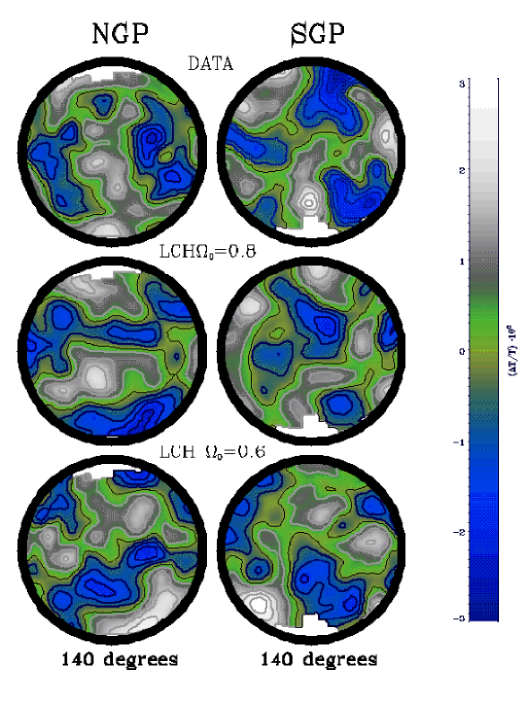
FIG. 10.: The figure consists of a column of three CMB sky-maps, each showing a pair of $140^{\circ}$ diameter hemispherical caps, centered on the South (SGP) and North (NGP) Galactic Poles, respectively. The top map labeled DATA shows the cobe–dmr 53+90+31 GHz A+B data after Wiener filtering, assuming a best-fit standard CDM model, normalized to the cobe–dmr amplitude. The next two maps are of one random realization of the CMB anisotropy in v3543(2,3) – our choice of a $L(arge)CH$ model example, for $\Omega_{0}=0.6~{}\&~{}0.8$ based on our theoretical calculations of $C(\hat{q},\hat{q}^{\prime})$ convolved with the cobe–dmr beam. Both surface and integrated (ISW) Sachs-Wolfe effects have been included in $C(\hat{q},\hat{q}^{\prime})$. No noise was added. The amplitude in each model was chosen to best-match the cobe–dmr data. The theoretical sky was Wiener-filtered using the cobe–dmr experimental noise to facilitate visual comparison with the data. LCH with $\Omega_{0}=0.8$ is compatible with the data with a suitable choice of orientation, whereas with $\Omega_{0}=0.6$, it is ruled out (See Table I). For all the maps in Figs. 10 and 11, the average, dipole and quadrupole determined for this cut sky were removed. A $20^{\circ}$ Galactic latitude cut was used, with extra pixel cuts to remove known regions of Galactic emission proposed by the cobe–dmr team, accounting for the ragged edges. The contours are linearly spaced at $15~{}\mu{\rm K}$ steps. The maps have been smoothed by a $1.66^{\circ}$ Gaussian filter.

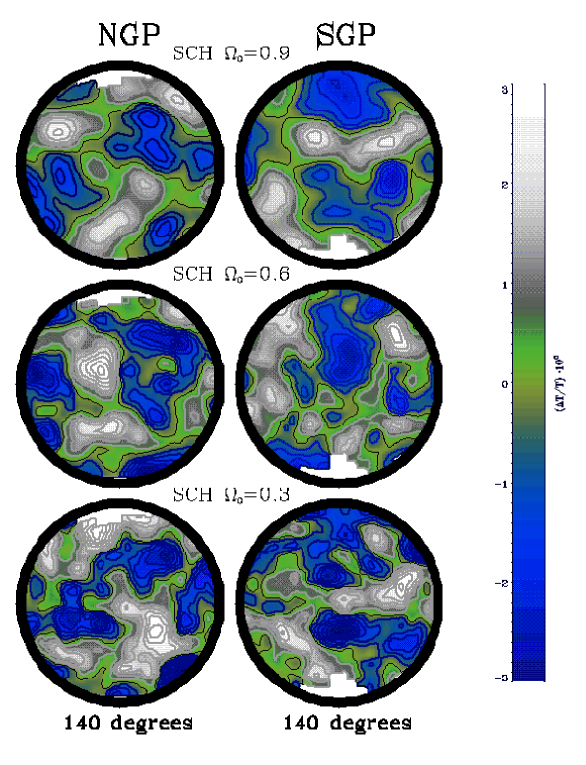
FIG. 11.: The three CMB sky-maps, each showing a pair of $140^{\circ}$ diameter hemispherical caps, centered on the South (SGP) and North (NGP) Galactic Poles, are analogous to the lower two plots in Fig. 10 but for the $S(mall)CH$ model m004(-5,1). The fact that $\Omega_{0}=0.3~{}\&~{}0.6$ models above are strongly ruled out by the cobe–dmr data is obvious visually. The $\Omega_{0}=0.9$ model is not obviously excluded on the visual basis, but is indeed excluded on the basis of our Bayesian analysis. (See Table I.)

VI Conclusion

Although there are an infinite number of possible CH spaces, one can extrapolate some general conclusions on CH universe models from our limited exploration of cobe–dmr constraints on the $LCH$ and $SCH$ examples. We shall present the CMB constraints on a larger set of CH spaces in [13]. The main CMB feature of small compact universe models – the presence of high correlations between many well-separated pixel pairs – is also their handicap. The cobe–dmr data does not, generally, favor interpretation as being a noisy random realization derived from a small compact model. Formally, the likelihood ${\cal P}(\bar{\Delta}_{\sc cobe-dmr}|C_{Tpp^{\prime}})$ is much smaller for such models than for a standard oCDM theory in which $C_{Tpp^{\prime}}$ mostly just falls off with separation between the pixels.

High correlations at large angles are numerous in a compact space with $d_{\cal M}<R_{\sc ls}$ and we are confident in concluding that such topologies are not viable models for our Universe in view of the cobe–dmr data. Of course, the possibility of exceptions in the infinite list of CH models remains, but the bulk of models must satisfy the, in our opinion quite solid, limit $d_{\cal M}>\alpha R_{\sc ls}$ to pass the CMB test. Setting $\alpha=1$ would be a very conservative choice; all our numerical simulations are consistent with at least $\alpha=1.4$. At this limiting value the CH models we tested are excluded at $3\sigma$ level.

Similar conclusions were reached by some of the authors (JRB, DP and Igor Sokolov [12]) for flat toroidal models. Comparison of the full angular correlation (computed using the eigenfunction expansion) with the cobe–dmr data led to a much stronger limit on the compactness of the universe than limits from other methods [33, 34]. The main result of the analysis was that $R_{T}/R_{\sc ls}>1.3$ at $95\%~{}CL$ for the equal-sided $3$-torus (with the periodicity length $2R_{T}$, the diameter of the torus is $d_{T}=3^{1/2}R_{T}$, thus $\alpha=2.25$ ). For $3$-tori with only one short dimension (or for the non-compact $1$-torus), the constraint on the most compact dimension is not quite as strong because the features can be hidden in the “zone of avoidance” associated with the Galactic cut.

Statistical properties of fluctuations in CH manifolds are anisotropic and inhomogeneous. CMB predictions of course depend not only on the topology of the space, but also on the position of the observer and the orientation of the Dirichlet domain with respect to cobe–dmr sky. This lack of high symmetry is reflected, in particular, in $R_{>}$ and $R_{<}$, which are not invariant under the choice of the space basepoint (i.e., the observer position) and which quantify how the sky looks for a given observer. Our limit on CH models uses the invariant linear measure $d_{\cal M}$, but roughly corresponds to the condition $R_{>}>R_{\sc ls}$ when $R_{>}$ is the outradius for the observer at the basepoint which maximizes the ‘injectivity radius’ of the space [19]. This means that when the Dirichlet domain just fits into the last-scattering sphere, the correlation matrix is already too distorted to satisfy the data. Moving the observer to another point, will generally increase $R_{>}$, but will also squash the domain in some other directions. In the more anisotropic view of the CH space presented to such an observer, we expect to predict less favorable CMB skies. Thus, moving the observer away from the basepoint which maximizes the ‘injectivity radius’ may not relax the constraint. The absence of good data close to the galactic plane, (i.e., the galactic cut in the data) may help some models at specific orientations, but not to the extent that it does for the $1$-torus space, which has an exact planar symmetry. Extensive analysis of the changes induced by varying observers is left to future work.

As we emphasized in [1, 2] and here, the constraints arise predominantly from predicted pattern mismatches in our models compared with the COBE tapestry. This is entirely encoded in $C_{Tpp^{\prime}}$, which can also be expressed in terms of a $Y_{\ell m}$ basis. However, $C_{T\ell m,\ell^{\prime}m^{\prime}}$ is generally quite complex and reducing consideration to the isotropized ${\cal C}_{\ell}$ loses a substantial amount of information, since it involves a $\delta_{\ell\ell^{\prime}}$ projection, followed by a trace over $m$. More importantly, as we show in detail in Appendix B, ${\cal C}_{\ell}$ has substantially increased error bars from “cosmic variance”, i.e., in the expected theoretical fluctuations about the mean, so we can draw only extremely weak conclusions about the model. This is evident in the error bars on the angular power spectrum shown for a set of the CH models in Figure 12. Thus, although the ${\cal C}_{\ell}$ for a compact model may fit the data reasonably well, and it sometimes does so even better than the corresponding infinite model with the same $\Omega_{0}$, statistically this may be a rather meaningless observation, and, if one is not careful, even misleading. Some authors [38, 37] have argued that because the mean ${\cal C}_{\ell}$ shape may look better visually, this is evidence that the models are preferred.

To make the point quantitatively that conventional use of ${\cal C}_{\ell}$ can lead to very wrong conclusions, Table II compares the likelihood ratios for a few models obtained using just ${\cal C}_{\ell}$ information, treated as if they were statistically isotropic Gaussian models with the the isotropized power spectrum, with what was obtained in Table I when the full pattern-recognition statistical treatment was made. Details on the construction of the Table are given in Appendix B. In all cases shown, the CH ${\cal C}_{\ell}$ is preferred over the ${\cal C}_{\ell}$ of the corresponding infinite model, but it is grossly misleading because of the enhanced error bars, and the huge amount of relevant information left out. All models are strongly ruled out, save one. And that manifold, with its specific orientation relative to the sky, is preferred even more than the statistically-isotropized one.

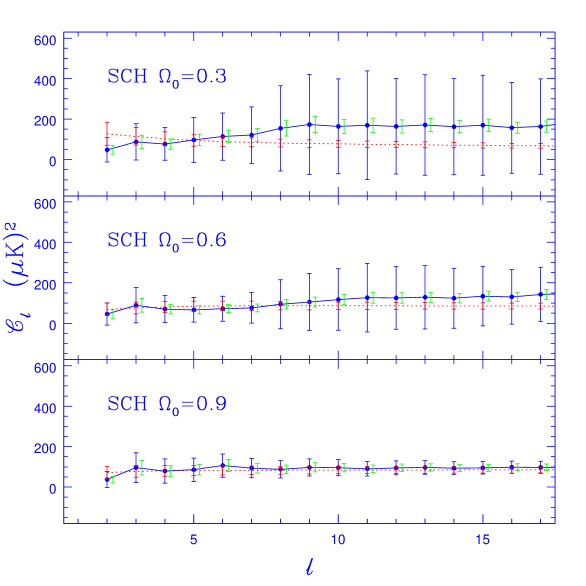
FIG. 12.: The three panels show angular power spectra for the SCH model at $\Omega_{0}=0.3$, $0.6$ and $0.9$, respectively. The larger error bars are the actual cosmic variance computed using the full correlation matrix information. The smaller error bars drawn slightly displaced to the right are the cosmic variance one would assign if one naively assumed that the ${\cal C}_{\ell}$ contained all the information. The excess variance reflects the incompleteness of the ${\cal C}_{\ell}$ information due to the inherent statistical anisotropy. The dotted (red) curve shows ${\cal C}_{\ell}$ for the simply connected ‘open’ universe at the same value of $\Omega_{0}$. The error bars show the cosmic variance. The ${\cal C}_{\ell}$ is normalized to give the same r.m.s. power as the corresponding SCH model for the cobe–dmr beam. The full cobe–dmr beam, with rough Gaussian scale $\sigma_{\rm beam}^{-1}\sim 17.5$, has been factored out in making the plot.

TABLE II.: The Log-likelihoods of the compact hyperbolic models relative to the infinite models with the same $\Omega_{m}$ are listed. The probabilities are calculated by confronting the models with the cobe–dmr data solely in terms of ${\cal C}_{\ell}$. For easy reference the corresponding relative likelihood for the “best” orientation is listed from Table I.

CH Topology	SCH: m004(-5,1)			LCH: v3543(2,3)
$\Omega_{m}$	0.3	0.6	0.9	0.6	0.8
Log. Likelihood Ratio	0.62(1.1$\sigma$)	0.43(0.93$\sigma$)	0.48(0.98$\sigma$)	0.61(1.1$\sigma$)	0.82(1.3$\sigma$)
Using only ${\cal C}_{\ell}$
Log. Likelihood Ratio	-35.5(8.4$\sigma$)	-22.9 (6.8$\sigma$)	-4.4(3.0$\sigma$)	-3.6(2.7$\sigma$)	2.5(2.2$\sigma$)
Using full $C_{Tpp^{\prime}}$ (“Best” orientation)

Most astrophysical observations point to a matter density $\Omega_{m}\mathrel{\hbox to0.0pt{\lower 3.0pt\hbox{$\mathchar 536\relax$}\hss}\raise 2.0pt\hbox{$\mathchar 316\relax$}}0.4$ [9]. For the matter-dominated $\Omega_{0}=\Omega_{m}$ open cosmology, when we combine this with the $d_{\cal M}>\alpha R_{\sc sls}$ cobe–dmr constraint that we suggest, i.e., $\Omega_{m}>1-{\rm tanh}^{2}\left(d_{\cal M}/2\alpha d_{c}\right)$, we would be able to rule out topologically small CH models with $d_{\cal M}/d_{c}\mathrel{\hbox to0.0pt{\lower 3.0pt\hbox{$\mathchar 536\relax$}\hss}\raise 2.0pt\hbox{$\mathchar 316\relax$}}2.8$ (adopting the conservative $\alpha=1.4$).

Recent SNIa results [10], the emerging location of a peak in the CMB power spectrum at $\ell\sim 200$, and the combination of CMB with large scale structure data [11] all point to a significant $\Omega_{\Lambda}$ term, with less room for a small $\Omega_{0}=\Omega_{m}+\Omega_{\Lambda}$, even though $\Omega_{m}$ may be small. Ironically, although this makes open models less attractive, having a non-zero $\Omega_{\Lambda}$ which combines with $\Omega_{m}$ to give $\Omega_{0}$ near unity actually returns topologically small CH spaces back to life, since it alleviates the constraint on the size $d_{\cal M}$. Qualitatively, CH models with the same value of $R_{\sc ls}/d_{c}$ will have similar constraints, whether there is $\Omega_{\Lambda}$ or not. Some quantitative differences will of course arise because of the diminished contribution from the ISW effect in the $\Omega_{m}+\Omega_{\Lambda}$ model compared to the corresponding $\Omega_{\Lambda}=0$ one.

In Figure 13 we show the $\Omega_{m}-\Omega_{\Lambda}$ parameter space, where the lines of constant $R_{\sc ls}/d_{c}$ provide rough limits on the viability of the CH models, depending on its size. This plot illustrates that allowing for nonzero $\Omega_{\Lambda}$ relaxes the limits on the allowed CH topology. This is a welcome conclusion, since one could argue that (topologically) small CH spaces are less complex and may be more probable for quantum processes in the early Universe to have created them, making them a more natural choice among other CH models [35].

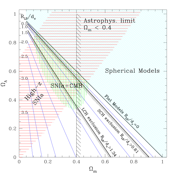
FIG. 13.: In the $\Omega_{m}-\Omega_{\Lambda}$ parameter plane, the horizontally shaded area shows the 95% CL (confidence limit) region coming from the analysis of high redshift supernovae SNIa [10]. For reference, the vertically shaded region shows 95% CL restrictions arising in the standard infinite universes when SNIa and CMB data are combined. Since intermediate-scale CMB data dominates the CMB constraint on the first peak position and hence on $\Omega_{0}$, where the influence of the topology would not be so important, the limits on $\Omega_{m},\Omega_{\Lambda}$ in CH spaces should be similar to those shown. We suggest that lines of constant $R_{\sc ls}/d_{c}$ would provide effective guides to the viability of the compact models. The two lines with enhanced weight correspond to the line $R_{\sc ls}/d_{c}=d_{\cal M}/1.4$ in our SCH and LCH example spaces. The allowed region is to the right of the $R_{\sc ls}/d_{c}=d_{\cal M}/1.4$ lines. The vertical line at $\Omega_{m}=0.4$ cuts out the high matter density part of the plane which is disfavored by observations.

Although our results strongly indicate that manifolds with small $R_{>}<R_{\sc ls}$ are unlikely to survive confrontation with the cobe–dmr data, we emphasize that, in the $R_{>}>R_{\sc ls}>R_{<}$ regime, there is some room both to have interesting specific CH correlation patterns and still be consistent with the cobe–dmr data. When $R_{<}$ is large compared to $R_{\sc ls}$, the results will quickly converge towards the usual infinite hyperbolic manifold results. The intermediate terrain still encompasses ample scope for interesting topological signatures to be discovered within the CMB. Although our methods are quite general, testing all manifolds in the SnapPea census this way is rather daunting, and there are countably infinite manifolds not yet prescribed. What may be promising for discovery are specialized statistical indicators, which are less powerful discriminators than the full Bayesian approach we have used here, but not as manifold sensitive; e.g., the statistical techniques which exploit the high degree of correlation along circle pairs that [28] have emphasized, and Fig. 5 reveals. Maps like we have constructed will be necessary to test the statistical significance of such methods. We also note that dramatically increasing the resolution beyond that of cobe–dmr , to e.g. MAP resolution, is quite feasible with current computing power using our techniques.

VII Acknowledgements

We have made extensive use of the SnapPea package and related material on compact hyperbolic spaces, which is available at the public website of the Geometry center at the University of Minnesota. TS acknowledges support during the final stages of this work from NSF grant EPS-9550487 with matching support from the state of Kansas. In the course of this project we have had enjoyable interactions with Janna Levin, Neil Cornish, Dave Spergel, Igor Sokolov, Glen Starkman and Jeff Weeks.

A Incorporating small angle CMB anisotropy

In this section, we discuss the calculation using the method of images of the primary CMB anisotropy at smaller angular scales where sources other than the Sachs-Wolfe effect make the dominant contribution. The most important effects are the Doppler shift due to scattering of photons on free electrons during recombination, and a term describing the compression and rarefaction of photons.

We shall consider only the scalar mode of perturbations. As in the main text of this paper, we choose to work in the longitudinal gauge in which the metric perturbations are described by two scalar potentials $\Phi$ and $\Psi$

$$ds^{2}=a^{2}(\tau)\left[\left(1+2\Phi\right)d\tau^{2}-(1-2\Psi)g^{(3)}_{ik}dx^{i}dx^{k}\right]\,.$$ (A1)

This gauge is particularly suitable for the analysis of multiply connected universes, since the perturbed 3-space is explicitly conformal to the background 3-space, leaving the topological identification of points in the background coordinates $x^{i}$ exact. Also for the perturbed quantities in the longitudinal gauge one does not need to distinguish between gauge-specific and gauge-invariant definitions.

In first-order perturbation theory, the photons observed at the origin from the direction $\hat{q}$ at the (present) moment $\tau_{0}$ have propagated along radial null-geodesics. The position $(\tau,x^{i})$ on the geodesics is parametrized by $(\tau_{0}-\chi,\chi\hat{q})$ in terms of the affine parameter $\chi$ with $\chi=0$ at the origin. $\tau_{0}$ coincides with the present radius of the FRW horizon, $\chi_{H}$.

The transport of the temperature fluctuation $\Delta_{T}(\tau,x^{k},\hat{q})$ along the photon path is given by the Boltzmann equation

$$-{\cal D}_{\chi}\Delta_{T}+(\partial_{\chi}\zeta)\,\Delta_{T}=\left(\partial_{\tau}\Psi+\hat{q}^{i}\partial_{i}\Phi\right)+(\partial_{\chi}\zeta)\,\left(\varepsilon/4+\hat{q}^{i}\partial_{i}{\psi_{v}}\right),~{}~{}~{}~{}{\cal D}_{\chi}=\hat{q}^{i}\partial_{i}-\partial_{\tau}\,,$$ (A2)

where we have used the following notations : ${\cal D}_{\chi}$ is the total derivative along the photon path and $\partial$ denotes the partial derivatives. Along the path the direction of the photon momentum $\hat{p}$ is opposite to the direction of $\hat{q}$. The energy density fluctuations are given by local angle averaging over momentum directions $\varepsilon(\tau,x^{i})=\int d\Omega_{\hat{p}}\Delta_{T}(\tau,x^{i},\hat{p})/4\pi$. The function $\zeta(\chi)=\int_{0}^{\chi}d\chi\sigma_{T}n_{e}$ is the optical depth due to Thompson scattering of photons on free electrons with a number density $n_{e}$. The velocity is described by the velocity potential $\psi_{v}$. We have also omitted subdominant terms related to the effects of polarization and the angular anisotropy in the scattering [36].

The resulting temperature fluctuation measured by the observer in the direction $\hat{q}$ is obtained by integrating eq. (A2) along the photon path

$$\Delta_{T}(\tau_{0},\hat{q})=\int_{0}^{\tau_{0}}{\mathrm{D}}\chi\,\left[\left(\partial_{\tau}\Psi+\hat{q}^{i}\partial_{i}\Phi\right)\,e^{-\zeta(\chi)}-\left(\epsilon/4+\hat{q}^{i}\partial_{i}\psi_{v}\right)\partial_{\chi}e^{-\zeta(\chi)}\right]\,.$$ (A3)

Assuming the standard recombination history, the approximation of ‘instant recombination’ is quite accurate for the CMB anisotropy at large and intermediate angular scales. It assumes an instantaneous transition from the phase at $\tau<\tau_{\sc ls}$, where the photons were tightly coupled with the electrons, to the phase at $\tau>\tau_{\sc ls}$ where they propagate freely after last scattering at $\tau_{\sc ls}$. In eq. (A3) this formally corresponds to the limit for the visibility function $e^{-\zeta(\chi)}\to\Theta(\tau_{0}-\tau_{\sc ls}-\chi)$, where $\Theta(x)$ is the Heaviside step function. Correspondingly, the differential visibility function $-\partial_{\chi}e^{-\zeta(\chi)}\to\delta(\tau_{0}-\tau_{\sc ls}-\chi)$, where $\delta(x)$ is the delta function. Omitting the monopole terms, one obtains the well known expression for temperature fluctuations in this limit:

$$\Delta_{T}(\tau_{0},\hat{q})=\left(\epsilon/4+\Phi+\hat{q}^{i}\partial_{i}\psi_{v}\right)\left|{}_{\stackrel{{\scriptstyle{\scriptstyle\tau=\tau_{\sc ls}}}}{{\chi=\tau_{0}-\tau_{\sc ls}}}}\right.+\int_{0}^{\tau_{0}-\tau_{\sc ls}}{\cal D}\chi\,\partial_{\tau}\left(\Psi+\Phi\right).$$ (A4)

The above expression for the CMB temperature fluctuation includes the Doppler term $\hat{q}^{i}\partial_{i}\psi_{v}$ in addition to the Sachs-Wolfe contribution given in eq. (2). To obtain the Sachs-Wolfe contribution in the form of eq. (2), the relation $\Phi=\Psi$ valid in the (fairly good) hydrodynamic approximation to the matter content in the universe is used. Furthermore, the well known solution to the evolution equations for the perturbations imply $\varepsilon(\tau_{\sc ls})\approx-8\Phi(\tau_{\sc ls})/3$ in the Sachs-Wolfe regime.

We have presented these well known results to stress that, in full generality, the CMB anisotropy can be expressed as a line of sight integral over a source function given purely in the real space. Thus, in a multiply-connected Universe the method of images can be directly applied to full CMB calculations in a similar manner as we have used it to calculate Sachs-Wolfe contribution.

The new element that eq. (A3) has beyond the Sachs-Wolfe expression of eq. (2) is the vectorial terms in the source function. For the scalar perturbations all of them are spatial derivatives of the potentials along the line of sight and can be reduced to time derivatives through integration by parts. Indeed, $\hat{q}^{i}\partial_{i}\Phi$ is readily converted into a $\partial_{\tau}\Phi$ addition to the integral plus the surface term $\Phi[\tau_{\sc ls},(\tau_{0}-\tau_{\sc ls})\hat{q}]$, as was implicitly done both in eq. (A4) and in eq. (2) in the main text. The Doppler term can also be dealt with the same way, however there is no obvious advantage of doing that. The reason is the $\delta$-function like, rather than step-function like, nature of the differential visibility multiplier in the Doppler term. Integration by parts gives an integral term with $\partial^{2}_{\chi}e^{-\zeta(\chi)}$, which quickly changes sign; and having to integrate it numerically may not indeed be a simplification over numerical differentiation.

As is clear in the simplifying instant recombination approximation, the Doppler term depends on the line-of-sight projection of a vector at last-scattering surface and not a scalar. As for a scalar field, a vector field on a multiply connected universe ${\cal M}^{u}/\Gamma$, can be expressed as a sum over images of the vector field on the universal cover, ${\cal M}^{u}$. However, in contrast to scalar fields, the discrete group $\Gamma$ acts both on the spatial position ${\bf x}$ and the vector at that point, i.e., the vector at the image point $\gamma[{\bf x}]$ is rotated relative to the vector at ${\bf x}$; and its projection on the line-of-sight is not preserved. Thus, at scales where it is dominant, the presence of the Doppler term at the last-scattering surface will tend to destroy the nice circle correlations that appear for the NSW case (see $\S$ IV A).

However, the presence of vector terms is not an obstacle for the numerical implementation of the method of images. Indeed, it is quite straightforward to implement the method of images to calculate the CMB correlation function for eq. (A4) or eq. (A3). For a completely general source term, the correlation function for the CMB anisotropy is the double integral

$$C(\hat{q},\hat{q}^{\prime})=\int_{0}^{\chi_{\!{}_{\rm H}}}d{\chi_{\!{}_{\rm 1}}}~{}\int_{0}^{\chi_{\!{}_{\rm H}}}d{\chi_{\!{}_{\rm 2}}}~{}\langle{\cal S}(\hat{q}{\chi_{\!{}_{\rm 1}}}){\cal S}(\hat{q}^{\prime}{\chi_{\!{}_{\rm 2}}})\rangle\,.$$ (A5)

In a compact (more generally, multiply connected) FRW universe, the method of images can be invoked to compute the source correlation function as a regularized sum over images over the source correlation function on the universal cover:

$$\langle{\cal S}(\hat{q}{\chi_{\!{}_{\rm 1}}}){\cal S}(\hat{q}^{\prime}{\chi_{\!{}_{\rm 2}}})\rangle^{c}=\widetilde{\sum_{\gamma\in\Gamma}}\langle{\cal S}(\hat{q}{\chi_{\!{}_{\rm 1}}})\gamma[{\cal S}(\gamma[\hat{q}^{\prime}{\chi_{\!{}_{\rm 2}}}])]\rangle^{u}$$ (A6)

where the superscripts $c$ and $u$ refer to the quantity in the multiply connected space and its universal cover, respectively. Tilde refers to the possible need for regularization. $\Gamma$ is the discrete subgroup of motions which defines the multiply connected space and $\gamma[{\bf x}]$ is the spatial point on the universal cover obtained by the action of the motion $\gamma\in\Gamma$ on the point ${\bf x}$. The important point to note is that one needs to implement the action of the motion $\gamma$ on the source function unless all the terms in the source function are scalar quantities (as was the case for the Sachs-Wolfe effect that we considered in this paper) when the action is trivial.

In summary, the CMB anisotropy correlation in a multiply connected universe can be computed in full generality using the method of images on the correlation function for CMB anisotropy source terms. However, it is important to identify the scalar, vector and tensor parts of the source functions and the action of the discrete motion has to be applied to non-scalar components of the source function.

B Inadequacy of ${\cal C}_{\ell}$ comparison for compact universes

In this appendix, we use the examples of the CH spaces we have studied here to discuss the limitations of a comparison of CMB anisotropy predictions to data solely in terms of the angular power spectrum for compact universe models.

The (isotropized) angular power spectrum, ${\cal C}_{\ell}$, widely used to summarize the CMB anisotropy predictions of a theoretical model, is defined by

$${\cal C}_{\ell}\equiv\frac{\ell(\ell+1)}{2\pi(2\ell+1)}~{}\sum_{m=-\ell}^{\ell}\langle\hat{a}_{\ell m}\hat{a}^{*}_{\ell m}\rangle,\quad{\rm where}\quad\hat{a}_{\ell m}=\int d\Omega_{\hat{q}}\,\widehat{\frac{\Delta T}{T}}(\hat{q})\,Y_{\ell m}(\hat{q})\,.$$ (B1)

The $\langle\,\rangle$ denotes an ensemble average of the random variable enclosed. In full generality, the expectation values of the pair products of the spherical harmonic coefficients $\langle\hat{a}_{\ell m}\hat{a}^{*}_{\ell^{\prime}m^{\prime}}\rangle$ are related to the correlation function $C(\hat{q},\hat{q}^{\prime})$ by

$$\langle\hat{a}_{\ell m}\,\hat{a}^{*}_{\ell^{\prime}m^{\prime}}\rangle=\int d\Omega_{\hat{q}}\int d\Omega_{\hat{q}^{\prime}}\left\langle\frac{\Delta T}{T}(\hat{q})\frac{\Delta T}{T}(\hat{q}^{\prime})\right\rangle Y_{\ell m}(\hat{q})Y^{*}_{\ell^{\prime}m^{\prime}}(\hat{q}^{\prime})=\int d\Omega_{\hat{q}}\int d\Omega_{\hat{q}^{\prime}}\,C(\hat{q},\hat{q}^{\prime})\,Y_{\ell m}(\hat{q})\,Y^{*}_{\ell^{\prime}m^{\prime}}(\hat{q}^{\prime})\,.$$ (B2)

In comparing theoretical predictions to observations, the power spectrum, ${\cal C}_{\ell}$, is a useful “data compression” of the $N(N+1)/2$ numbers in the $N\times N$ correlation matrix, $C_{T}$, into $\approx N$ multipoles values of ${\cal C}_{\ell}$ . However, it is sometimes overlooked (see e.g., [38, 37]) that a necessary condition for this compression to be “loss free” is that the CMB fluctuations are statistically isotropic, i.e., the ensemble averages such as $C(\hat{q},\hat{q}^{\prime})$ or $\langle\hat{a}_{\ell m}\hat{a}^{*}_{\ell m}\rangle$ are invariant under rotation.

The standard (simply connected, FRW) universe models respect global isotropy and predict a statistically isotropic CMB sky. The full angular correlation function $C(\hat{q},\hat{q}^{\prime})$ between two directions is then solely a function of their separation, $\hat{q}\cdot\hat{q}^{\prime}$. Using eq.(B2), the equivalent statement is that $\langle\hat{a}_{\ell m}\hat{a}^{*}_{\ell^{\prime}m^{\prime}}\rangle=2\pi{\cal C}_{\ell}/(\ell(\ell+1))\,\delta_{\ell\ell^{\prime}}\,\delta_{mm^{\prime}}$, is diagonal in the $(\ell,m)$ space and independent of $m$. The angular power spectrum ${\cal C}_{\ell}$ is uniquely related to the correlation function through the expansion (6) and contains the same information.

All Euclidean or Hyperbolic compact spaces violate global isotropy and the CMB temperature fluctuations are statistically anisotropic, i.e., $C(\hat{q},\hat{q}^{\prime})\not\equiv C(\hat{q}\cdot\hat{q}^{\prime})$. As a consequence, the $\langle\hat{a}_{\ell m}\hat{a}^{*}_{\ell^{\prime}m^{\prime}}\rangle$ now define the relevant angular power spectra, and these are are no longer required to be diagonal and independent of $m$. Thus, ${\cal C}_{\ell}$ as defined by eq. (B1) misses both off-diagonal pair products of $a_{\ell m}$’s and isotropizes further by summing up the $m$-dependent diagonal $a_{\ell m}$ pair products.

Figure 14 shows the normalized full angular power spectrum

$$\rho_{\ell m}^{\ell^{\prime}m^{\prime}}\equiv\langle\hat{a}_{\ell m}\,\hat{a}^{*}_{\ell^{\prime}m^{\prime}}\rangle/\sqrt{\langle\hat{a}_{\ell m}\,\hat{a}^{*}_{\ell m}\rangle\langle\hat{a}_{\ell^{\prime}m^{\prime}}\,\hat{a}^{*}_{\ell^{\prime}m^{\prime}}\rangle}$$ (B3)

for all the $(\ell,m)$ with $2\leq\ell\leq 10$ for the CH models considered in our paper. This cross correlation coefficient clearly shows the the existence of significant off-diagonal $\langle\hat{a}_{\ell m}\,\hat{a}^{*}_{\ell^{\prime}m^{\prime}}\rangle$ in the m004(-5,1) at $\Omega_{0}=0.3$ where $\rho_{\ell m}^{\ell^{\prime}m^{\prime}}$ ranges between $-0.5$ up to $0.6$. This is the most extreme case in our set of models since it has the smallest size of the SLS relative to the Dirichlet domain ($V_{\rm LS}/V_{\!\cal M}=153.4$) amongst the models discussed in this paper. As $V_{\rm LS}/V_{\!\cal M}$ decreases, the number of $(\ell,m)$ pairs with high $\rho_{\ell m}^{\ell^{\prime}m^{\prime}}$ decreases and the $\langle\hat{a}_{\ell m}\,\hat{a}^{*}_{\ell^{\prime}m^{\prime}}\rangle$ matrix becomes closer to diagonal. However, for the same CH space the range of $\rho_{\ell m}^{\ell^{\prime}m^{\prime}}$ remains comparable, e.g., for m004(-5,1) at $\Omega_{0}=0.9$ ($V_{\rm LS}/V_{\!\cal M}=1.2$), $\rho_{\ell m}^{\ell^{\prime}m^{\prime}}$ ranges from $-0.42$ to $0.5$ for $2\leq\ell\leq 10$. The larger CH v3543(2,3) model is more isotropic, the $\langle\hat{a}_{\ell m}\,\hat{a}^{*}_{\ell^{\prime}m^{\prime}}\rangle$ are somewhat more diagonal with most of the significant off-diagonal terms at low $\ell$. The ranges in $\rho_{\ell m}^{\ell^{\prime}m^{\prime}}$ are $\pm 0.29$ and $\pm 0.23$ for $\Omega_{0}=0.6$ and $0.8$, respectively. The $m$-dependence of the diagonal products $\langle\hat{a}_{\ell m}\hat{a}^{*}_{\ell m}\rangle$ is shown in Figure 15.

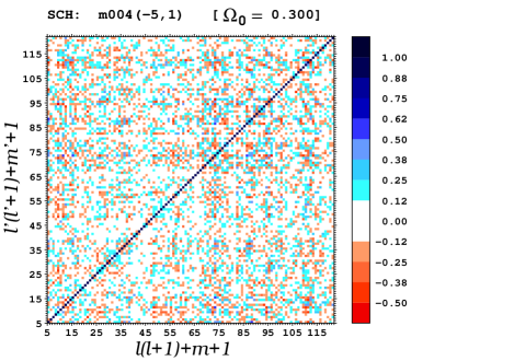
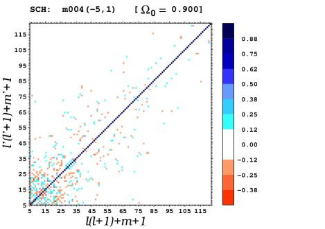
FIG. 14.: The figure demonstrates the nondiagonal nature of the expectation values of $a_{\ell m}$ pair products when the CMB anisotropy is statistically anisotropic using the examples of the SCH model at $\Omega_{0}=0.3$ (left panel) and $\Omega_{0}=0.9$ (right panel). We use a single positive integer index, $n=\ell(\ell+1)+m+1$ to uniquely represent each $(\ell,m)$. Each square represents a pair of $(\ell,m)$ spherical harmonic indices for all $(\ell,m)$ for $2\leq\ell\leq 10$. The cross correlation coefficient, $\rho_{\ell m}^{\ell^{\prime}m^{\prime}}\equiv\langle\hat{a}_{\ell m}\,\hat{a}^{*}_{\ell^{\prime}m^{\prime}}\rangle/\sqrt{\langle\hat{a}_{\ell m}\,\hat{a}^{*}_{\ell m}\rangle\langle\hat{a}_{\ell^{\prime}m^{\prime}}\,\hat{a}^{*}_{\ell^{\prime}m^{\prime}}\rangle}$ at a given $(n,n^{\prime})$ square is represented by the level of grey (or color) shown in the accompanying palette. (The squares corresponding to pairs with mild cross correlation, $|\rho_{\ell m}^{\ell^{\prime}m^{\prime}}|<0.12$, have been left blank to highlight the strong ones). For statistically isotropic CMB anisotropy only the diagonal $\rho_{\ell m}^{\ell m}=1$ terms will be nonzero. As expected, the CMB anisotropy in the SCH model is more isotropic at $\Omega_{0}=0.9$ as evident from the more diagonal nature of $\rho_{\ell m}^{\ell m}$ in the right panel.

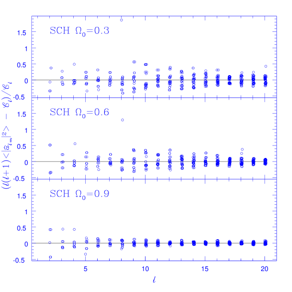
FIG. 15.: The three panels of the figure show the relative deviation of $\ell(\ell+1)\langle\hat{a}_{\ell m}\,\hat{a}^{*}_{\ell^{\prime}m^{\prime}}\rangle$ from the mean value ${\cal C}_{\ell}$ for all $(\ell,m)$ ( $2\leq\ell\leq 20$) in the SCH model at $\Omega_{0}=0.3$, $0.6$ & $0.9$, respectively. The non zero deviations demonstrate that the diagonal $\langle\hat{a}_{\ell m}\,\hat{a}^{*}_{\ell^{\prime}m^{\prime}}\rangle$ are not independent of $m$ when the CMB is statistically anisotropic. The relative deviations decrease with $\Omega_{m}$ as the space become larger relative to the SLS. The point with large deviation in the upper two panels corresponds to $(\ell,m)=(8,0)$.

For statistically anisotropic CMB fluctuations, the ${\cal C}_{\ell}$ contains less information than the full correlation matrix $C(\hat{q},\hat{q}^{\prime})$ independent of the underlying statistics. For concreteness, we now focus our discussion on Gaussian random CMB fluctuations which are completely specified by $C(\hat{q},\hat{q}^{\prime})$. For statistically anisotropic CMB, the incompleteness of the information contained in the ${\cal C}_{\ell}$ is reflected in the enhanced cosmic variance, $\langle{\cal C}_{\ell}^{2}\rangle$. Let us split the correlation matrix into an isotropic part determined by ${\cal C}_{\ell}$ through eq.(6) and an anisotropic term containing the remainder, i.e.,

$$C(\hat{q},\hat{q}^{\prime})=C^{\sc I}(\hat{q},\hat{q}^{\prime})+C^{\sc A}(\hat{q},\hat{q}^{\prime})$$ (B4)

so that, by definition, the isotropic part $C^{\sc I}(\hat{q},\hat{q}^{\prime})$ is described by the set of coefficients $C_{l}$ of Legendre series

$$C^{\sc I}(\hat{q},\hat{q}^{\prime})=\sum_{\ell}\frac{\ell+1/2}{\ell(\ell+1)}~{}{\cal C}_{\ell}P_{\ell}(\hat{q}\cdot\hat{q}^{\prime})\,,$$ (B5)

and the anisotropic part $C^{\sc A}(\hat{q},\hat{q}^{\prime})$ is orthogonal to the Legendre polynomials

$$\int d\Omega_{\hat{q}}\int d\Omega_{\hat{q}^{\prime}}\,C^{\sc A}(\hat{q},\hat{q}^{\prime})\,P_{\ell}(\hat{q}\cdot\hat{q}^{\prime})=0\,.$$ (B6)

The presence of the nonzero anisotropic part $C^{\sc A}(\hat{q},\hat{q}^{\prime})$ is the main attribute of statistically anisotropic models, and in particular of the CH models. Consider now the effect this term has on the probability distribution $P(\tilde{\cal C}_{\ell})$ of the isotropized power spectrum estimator

$$\tilde{\cal C}_{\ell}\equiv\frac{\ell(\ell+1)}{2\pi(2\ell+1)}~{}\sum_{m=-\ell}^{\ell}\int d\Omega_{\hat{q}}\int d\Omega_{\hat{q}^{\prime}}\frac{\Delta T}{T}(\hat{q})\frac{\Delta T}{T}(\hat{q}^{\prime})Y_{\ell m}(\hat{q})Y^{*}_{\ell m}(\hat{q}^{\prime})\,.$$ (B7)

Of course, the expectation value of the estimator is determined solely by $C^{\sc I}(\hat{q},\hat{q}^{\prime})$ (as it should be using eq.(B6)):

$$\langle\tilde{\cal C}_{\ell}\rangle=\frac{\ell(\ell+1)}{8\pi^{2}}\int d\Omega_{\hat{q}}\int d\Omega_{\hat{q}^{\prime}}\,C(\hat{q},\hat{q}^{\prime})\,P_{\ell}(\hat{q}\cdot\hat{q}^{\prime})\,.$$ (B8)

However, the distribution $P(\tilde{\cal C}_{\ell})$ depends on the anisotropic part $C^{\sc A}(\hat{q},\hat{q}^{\prime})$. In particular, the variance of $\tilde{\cal C}_{\ell}$, which can be calculated as a four-point correlation of the $\Delta T$’s, is enhanced due to the influence of $C^{\sc A}(\hat{q},\hat{q}^{\prime})$:

$${\rm var}(\tilde{\cal C}_{\ell})\equiv\langle\tilde{\cal C}_{\ell}^{2}\rangle-\langle\tilde{\cal C}_{\ell}\rangle^{2} = 2\left[\frac{\ell(\ell+1)}{8\pi^{2}}\right]^{2}\int d\Omega_{\hat{q}_{1}}\int d\Omega_{\hat{q}_{2}}\int d\Omega_{\hat{q}_{3}}\int d\Omega_{\hat{q}_{4}}\,C(\hat{q}_{1},\hat{q}_{3})P_{\ell}(\hat{q}_{1}\cdot\hat{q}_{2})\,C(\hat{q}_{2},\hat{q}_{4})\,P_{\ell}(\hat{q}_{3}\cdot\hat{q}_{4})$$ (B9)

$$= \frac{2\langle\tilde{\cal C}_{\ell}\rangle^{2}}{2\ell+1}+\frac{\ell^{2}(\ell+1)^{2}}{32\pi^{4}}\int d\Omega_{\hat{q}_{1}}\int d\Omega_{\hat{q}_{2}}\left[\int d\Omega_{\hat{q}_{3}}\,C^{\sc A}(\hat{q}_{1},\hat{q}_{3})\,P_{\ell}(\hat{q}_{2}\cdot\hat{q}_{3})\right]^{2}\,.$$ (B10)

In the final expression, the first term is the well known result for the cosmic variance of ${\cal C}_{\ell}$, strictly valid only for statistically isotropic CMB fluctuations. The second term was obtained using the fact that $C^{\sc A}(\hat{q}_{1},\hat{q}_{2})$ and $P_{\ell}(\hat{q}_{1}\cdot\hat{q}_{2})$ are symmetric functions. It represents a positive definite correction to the standard cosmic variance arising from the anisotropy of $C(\hat{q},\hat{q}^{\prime})$. Hence, the cosmic variance is always larger for a statistically anisotropic CMB compared to that expected for the statistically isotropic case with the same ${\cal C}_{\ell}$.

To calculate eq.(B10) numerically, we took our $C_{Tpp^{\prime}}$ and used matrix representations of the $P_{\ell}$ at the relevant COBE-pixel pairs. As a check of accuracy, the same procedure was applied to the infinite statistically isotropic models and the first term in eq.(B10) was recovered. This is a stringent test of the cancellations required to obtain this result. We found that for the finite compact models as well as the infinite models, our results are accurate for angular scales bigger than the beam, including the finite pixel effects.

Figure 12 shows the angular power spectrum for a set of the CH models with the associated cosmic variance. It demonstrates that the cosmic variance of ${\cal C}_{\ell}$ in CH models is significantly higher than one may naively assign assuming statistical isotropy. As a result, ${\cal C}_{\ell}$’s do not strongly distinguish CH models from the corresponding standard isotropic models and, on their own, are not very restrictive. Comparing CMB predictions of CH spaces to data using ${\cal C}_{\ell}$ alone is not incorrect, but inadequate since one has not used the full information available. The larger cosmic variance simply implies that the theoretical prediction is weaker. The argument that a comparison based on more information is more relevant is quite obvious. Any evaluation of the relative likelihood of a model based on ${\cal C}_{\ell}$ is superseded by a likelihood analysis that uses the complete correlation information. A model that does well solely in terms of ${\cal C}_{\ell}$ but fails in terms of the correlation matrix $C_{Tpp^{\prime}}$ should be considered ruled out.

In Table II we compare the relative likelihood for our models obtained using ${\cal C}_{\ell}$ versus that obtained using the full correlation information.

The procedure we use to determine the first line in the Table is to take the compact model’s $C_{Tpp^{\prime}}$, use the $P_{\ell}$ matrices to calculate the theoretical ${\cal C}_{\ell}$, as in eq.(B8), then assume that we have an infinite model with exactly that power spectrum, so that these ${\cal C}_{\ell}$’s encode all the information in the theory. We then use these to calculate new $C_{Tpp^{\prime}}$ for this theory, and determine the full Bayesian likelihood for it relative to the true infinite open model with the same $\Omega_{0}$ and its corresponding ${\cal C}_{\ell}$. The results show that at roughly the $+1\sigma$ level, these power spectra are preferred. Note that the likelihood ratios in row 1 are independent of orientation. However, the second row of the Table shows that when the full information on angular patterns is included in the analysis, the likelihoods change dramatically, strongly disfavouring small compact models, as in Table I. As well, the case for the $\Omega_{0}=0.8$ LCH model at the best orientation is enhanced by the inclusion of the full pattern information.

Models which fare very poorly with respect to a full correlation comparison may well look favored based on the ${\cal C}_{\ell}$. The reason for this is not hard to understand. If the compact space is not much larger than the SLS then it predicts strong anisotropic correlation features in the CMB sky which are at odds with the data (see $\S$ IV). However, an isotropized measure such as the ${\cal C}_{\ell}$ is insensitive to these features. This implies that the comparison of CMB anisotropy in CH models using ${\cal C}_{\ell}$ alone is grossly inadequate and could be quite misleading.

REFERENCES

- [1] J. R. Bond, D. Pogosyan and T. Souradeep, in: Proceedings of the XVIIIth Texas Symposium on Relativistic Astrophysics, ed. A. Olinto, J. Frieman, and D. N. Schramm, (World Scientific, 1997).
- [2] J. R. Bond, D. Pogosyan and T. Souradeep, Class. Quant. Grav. 15, 2671, (1998).
- [3] J. R. Bond, D. Pogosyan, and T. Souradeep in this volume (paper-I), (1998).
- [4] G. F. R. Ellis, Gen. Rel. Grav. 2, 7,(1971).
- [5] D. D. Sokolov and V. F. Shvartsman, Zh. Eksp. Theor. Fiz. 66, 412, (1974) [JETP, 39, 196 (1974)] and references therein to the early papers on ghost searches.
- [6] M. Lachieze-Rey and J. -P. Luminet, Phys. Rep. 25, 136, (1995).
- [7] J. R. Gott, Mon. Not. R. Astr. Soc. 193, 153, (1980).
- [8] N.J. Cornish, D. N. Spergel and G. D. Starkman, Phys. Rev. Lett. 77, 215, (1996).
- [9] A. Dekel, D. Burstein and S. D. M. White, 1996, in Critical Dialogues in Cosmology, ed. N.Turok, World Scientific; D. N. Spergel, Class. Quant. Grav. 15, 2589, (1998); N. Bahcall and X. Fan, preprint (astro-ph/9804082).
- [10] S. Perlmutter, et al. , preprint: astro-ph/9812133 (To appear in Astrophys. J. 516), (1998); D. Schmidt,et al. , Astrophys. J., 507, 46 (1998); A. G. Riess, et al. , (preprint: astro-ph/9805201) (To appear in Astron. J.).
- [11] J. R. Bond and A. H. Jaffe, Phil. Trans. R. Soc. London 357, 57-75 (1999).
- [12] J. R. Bond, in Proc. of the XVIth Moriond Astrophysics Meeting, ed. F. R. Bouchet et al. ., (Editions Frontieres, France, 1997); J. R. Bond, Proc. Natl. Acad. Sci. USA, 95, 35, (1998).
- [13] J. R. Bond, D. Pogosyan and T. Souradeep, in preparation.
- [14] V. F. Mukhanov, H. A. Feldman and R. H. Brandenberger, Phys. Rep. 215, 203, (1992).
- [15] M. L. Wilson, Astrophys. J., 253, L53, (1982).
- [16] N.J. Cornish, D. N. Spergel and G. D. Starkman, Phys. Rev. D57, 5982, (1998).
- [17] P. H. Berard, Spectral Geometry: Direct and Inverse Problems, Lec. Notes in mathematics, 1207, (Springer-Verlag, Berlin, 1980).
- [18] I. Chavel, Eigenvalues in Riemannian geometry, (Academic Press, 1984).
- [19] J. R. Weeks, SnapPea: A computer program for creating and studying hyperbolic 3-manifolds, Univ. of Minnesota Geometry Center (freely available at http://www.geom.umn.edu).
- [20] W. P. Thurston, The Geometry of 3-Manifolds, lecture notes, Princeton University (1979); W.P. Thurston and J. R. Weeks, Sci. Am. 251, 108, (1984).
- [21] D. Gabai, R. G. Meyerhoff and N. Thurston, preprint MSRI 1996-058, (1996).
- [22] J. R. Weeks,Ph.D. Thesis, (Princeton, 1985); S. V. Matveev and A. T. Fomenko, Usp. Mat. Nauk. 43, 5, (1988) [ Russ. Math. Surv. 43, 3, (1988)].
- [23] E. Harrison, Rev. Mod. Phys. 39, 862, (1967).
- [24] D. H. Lyth and E. D. Stewart, Phys. Lett. B252, 336, (1990).
- [25] B. Ratra and P. J. E. Peebles, Astrophys. J. Lett. 432, L5, (1994).
- [26] C. Bennett et al. , Ap. J. Lett.464, L1, (1996); and 4-year DMR references therein.
- [27] J. R. Bond, Phys. Rev. Lett., 74, 4369, (1994).
- [28] N.J. Cornish, D.N. Spergel & G. D. Starkman, Class. Quantum Grav., 15, 2657, (1998).
- [29] D. D. Sokoloff and A. A. Starobinski, Sov. Astron. 19, 629, (1975).
- [30] J. Levin, J. D. Barrow, E. F. Bunn and J. Silk, Phys. Rev. Lett. 79, 974, (1997).
- [31] A. H. Jaffe and J. R. Bond, in Proc. of the XVIth Moriond Astrophysics meeting, ed. F.R. Bouchet et al. ., (Editions Frontieres, France, 1997).
- [32] J. R. Bond, A. H. Jaffe and L. Knox, Phys. Rev. D 57, 2117, (1998).
- [33] A. A. Starobinsky, JETP Lett. 57, 622, (1993); A. de Oliveira Costa, G. F. Smoot and A. A. Starobinsky, Astrophys. J. 468, 457, (1996).
- [34] I. Y. Sokolov, JETP Lett. 57, 617, (1993); D. Stevens, D. Scott and J. Silk, Phys. Rev. Lett. 71, 20, (1993); A. de Oliveira Costa and G. F. Smoot, Astrophys. J. 448 477, (1995).
- [35] G. W. Gibbons, Class. Quantum Grav. 15, 2605, (1998).
- [36] J. R. Bond, Theory and Observations of the Cosmic Background Radiation, in Cosmology and Large Scale Structure, Les Houches Session LX, August 1993, ed. R. Schaeffer, (Elsevier Science Press, 1996).
- [37] K. T. Inoue, K. Tomita, N. Sugiyama, preprint, astro-ph/9906304
- [38] N. J. Cornish and D. N. Spergel, preprint, astro-ph/9906401; preprint, (math.DG/9906017).