Optical photometry of the UCM Lists I and II

Abstract

We present Johnson $B$ CCD photometry for the whole sample of galaxies of the Universidad Complutense de Madrid (UCM) Survey Lists I and II. They constitute a well-defined and complete sample of galaxies in the Local Universe with active star formation. The data refer to 191 S0 to Irr galaxies at an averaged redshift of 0.027, and complement the already published Gunn $r$, $J$ and $K$ photometries. In this paper the observational and reduction features are discussed in detail, and the new colour information is combined to search for clues on the properties of the galaxies, mainly by comparing our sample with other surveys.

1 Introduction

The Universidad Complutense de Madrid Survey (UCM Survey List I; Zamorano et al. Zam94 (1994), List II; Zamorano et al. Zam96 (1996)) constitutes a representative and fairly complete sample of current star-forming galaxies in the Local Universe (Gallego Gal99 (1999)). Its main purposes are to identify and study new young, low metallicity galaxies and to quantify the properties of the current star formation in the Local Universe. Another key goal was also to provide a reference sample for the studies of high-redshift populations, mainly dominated by star-forming galaxies.

The UCM Survey was carried out with the 80/120 cm f/3 Schmidt telescope at the German-Spanish Observatory of Calar Alto (Almería, Spain). A $4\degr$ full-aperture prism and a IIIaF photographic emulsion were the standard instrumental setup. The survey was able to detect emission line galaxies (ELG) to a Gunn $r$ magnitude limit of about 18^m; the objects were selected by the presence of H$\alpha$ $\lambda$6563 + [NII] $\lambda$6584 emission in their spectra. A total number of 191 objects were cataloged as UCM galaxies in List I and List II. A third list (UCM Survey List III; Alonso et al. Gar99 (1999)) will extend the sample around to 0.5^m fainter objects due to the implementation of a new fully automatic procedure for the detection and analysis of the objective-prism spectra.

The galaxies included in UCM lists I and II (hereafter the UCM survey) have been deeply analyzed in the Gunn $r$ bandpass (Vitores et al. 1996a and 1996b ), and also in the $J$ and $K$ nIR bands by Alonso-Herrero et al. (Alm96 (1996)) and Gil de Paz et al. (Gil99 (1999)). The spectroscopic analysis was performed by (Gallego et al. Gal96 (1996), Gal97 (1997)). It has also been used to deduce the H$\alpha$ luminosity function in the Local Universe (Gallego et al. Gal95 (1995)). The UCM sample is now widely used as reference for spectroscopic studies of high-$z$ populations (see the nice review by Madau Mad99 (1999)).

The UCM survey includes a total of 191 galaxies at an averaged redshift of 0.027. Morphologically, the sample is dominated by late-type spirals (around 47% being Sb or later) with less than 10% presenting typical parameters of earlier types and the remaining 10% being irregulars (Vitores et al. 1996a ). Spectroscopically, all types of star-forming galaxies previously known in the literature are represented; most of the UCM objects are low-excitation, high-metallicity starburst-like galaxies (57%) but there are also high-excitation, low-metallicity HII-like galaxies (32%). A fraction of AGN objects are also present (8%). Their metallicities range from solar values to $\frac{1}{40}Z_{\sun}$, peaking at $\frac{1}{4}Z_{\sun}$ (Gallego et al. Gal97 (1997)).

Photometrically, the UCM Survey was first imaged in the Gunn $r$ band due to the close relationship between this band and the one used in the primary photographic plates. In order to get colour information of this sample, we started a long-term project to obtain detailed $B$ band photometry. This band was selected with two main purposes: (1) obtaining an optical colour with a considerable base width, (2) getting information more directly comparable with high-redshift surveys.

In this paper we present $B$ band photometry for the whole sample and compare it with the previous optical data . In later papers we will perform the study of the disk and bulge components in the $B$-band and will combine the broad band data (both optical and nIR) with H$\alpha$ images in order to carry out a spatially resolved stellar population synthesis.

The paper is structured as follows: we introduce the sample of galaxies and the Johnson $B$ observations in Section 2. The galaxy photometry is afforded in Section 3. Statistics and the comparison with previous photometry are considered Section 4. Finally, we present the conclusions in Section 5. A Hubble constant $H_{0}$=50 km s^-1 Mpc^-1 and a deceleration parameter $q_{0}$=0.5 have been used throughout this paper.

2 Observations

2.1 The sample

The UCM sample of galaxies is divided into two lists. Galaxies of List I (Zamorano et al. Zam94 (1994)) and List II (Zamorano et al. Zam96 (1996)) were found in fields in a region of the sky from right ascension 12^h to 16^h and from 22^h to 2^h, respectively. The surveyed region covered a 10$\degr$ width strip centered at declination 20$\degr$ for both lists. A summary of the main features of each galaxy is listed in Table 1, including the names, redshifts, morphological and spectral types, Gunn $r$ magnitudes and $B-V$ colour excesses as obtained from the Balmer decrements.

Table 1: The sample of galaxies in the UCM Survey Lists I and II.

UCM name	$z$	MphT	SpT	mr	$E(B-V)$	UCM name	$z$	MphT	SpT	mr	$E(B-V)$
(1)	(2)	(3)	(4)	(5)	(6)	(1)	(2)	(3)	(4)	(5)	(6)
0000$+$2140	0.0238	-	HIIH	-	1.204	0141$+$2220	0.0174	Sb	DANS	15.67	0.742
0003$+$2200	0.0224	Sc$+$	DANS	16.16	0.867	0142$+$2137	0.0362	SBb	Sy2	14.19	0.537
0003$+$2215	0.0223	-	SBN	-	1.008	0144$+$2519	0.0414	SB(r)	SBN	14.78	1.033
0003$+$1955	0.0278	-	Sy1	-	-	0147$+$2309	0.0194	Sa	HIIH	15.82	0.486
0005$+$1802	0.0187	-	SBN	-	1.244	0148$+$2124	0.0169	BCD	BCD	16.32	0.174
0006$+$2332	0.0159	-	HIIH	-	0.644	0150$+$2032	0.0323	Sc$+$	HIIH	16.28	0.085
0013$+$1942	0.0272	Sc$+$	HIIH	16.39	0.276	0156$+$2410	0.0134	Sc$+$	DANS	14.55	0.702
0014$+$1829	0.0182	Sa	HIIH	16.01	1.473	0157$+$2413	0.0177	Sc$+$	Sy2	13.65	0.725
0014$+$1748	0.0182	SBb	SBN	14.13	0.806	0157$+$2102	0.0106	Sb	HIIH	14.39	0.474
0015$+$2212	0.0198	Sa	HIIH	15.59	0.215	0159$+$2326	0.0178	Sc$+$	DANS	14.72	-
0017$+$1942	0.0281	Sc$+$	HIIH	15.34	0.357	0159$+$2354	0.0170	Sa	HIIH	16.07	0.565
0017$+$2148	0.0189	-	HIIH	-	0.575	1246$+$2727	0.0199	-	HIIH	-	0.775
0018$+$2216	0.0169	Sb	DANS	15.82	0.136	1247$+$2701	0.0231	Sc$+$	DANS	15.97	0.515
0018$+$2218	0.0220	-	SBN	-	-	1248$+$2912	0.0217	-	SBN	-	0.715
0019$+$2201	0.0191	Sc$+$	DANS	15.54	0.438	1253$+$2756	0.0165	Sa	HIIH	15.09	-
0022$+$2049	0.0185	Sb	HIIH	14.45	0.901	1254$+$2741	0.0172	Sb	SBN	15.81	0.645
0023$+$1908	0.0251	-	HIIH	-	0.409	1254$+$2802	0.0253	Sc$+$	DANS	15.76	-
0034$+$2119	0.0315	-	SBN	-	0.684	1255$+$2819	0.0273	Sb	SBN	15.01	0.651
0037$+$2226	0.0204	-	SBN	-	0.615	1255$+$3125	0.0258	Sa	HIIH	15.07	0.409
0038$+$2259	0.0464	Sa	SBN	15.07	0.810	1255$+$2734	0.0234	Irr	SBN	15.99	0.715
0039$+$0054	0.0191	-	SBN	-	-	1256$+$2717	0.0273	-	DHIIH	-	0.447
0040$+$0257	0.0367	Sc$+$	DANS	16.76	-	1256$+$2732	0.0234	S0	SBN	15.40	-
0040$+$2312	0.0254	-	SBN	-	-	1256$+$2701	0.0247	Irr	HIIH	16.32	0.220
0040$+$0220	0.0173	Sb	DANS	16.39	0.378	1256$+$2910	0.0279	Sb	SBN	15.10	-
0040$-$0023	0.0142	LINER	-	-	-	1256$+$2823	0.0307	Sb	SBN	15.11	0.644
0041$+$0134	0.0169	-	-	-	-	1256$+$2754	0.0172	-	SBN	-	0.645
0043$+$0245	0.0180	-	HIIH	-	0.950	1256$+$2722	0.0287	Sc$+$	DANS	16.05	0.928
0043$-$0159	0.0161	-	SBN	-	-	1257$+$2808	0.0181	Sa	SBN	15.45	1.344
0044$+$2246	0.0253	Sb	SBN	14.83	1.384	1258$+$2754	0.0253	Sb	SBN	15.38	1.020
0045$+$2206	0.0203	-	HIIH	-	0.493	1259$+$2934	0.0239	Sb	Sy2	14.18	0.984
0047$+$2051	0.0577	Sc$+$	SBN	16.00	0.598	1259$+$3011	0.0307	Sa	SBN	15.36	0.682
0047$-$0213	0.0144	Sa	DHIIH	14.82	0.857	1259$+$2755	0.0235	Sa	SBN	14.45	0.913
0047$+$2413	0.0347	Sa	SBN	14.69	1.059	1300$+$2907	0.0219	Sb	HIIH	16.69	0.620
0047$+$2414	0.0347	-	SBN	-	0.592	1301$+$2904	0.0266	Sb	HIIH	15.18	0.207
0049$-$0006	0.0377	BCD	BCD	18.22	0.006	1302$+$2853	0.0237	Sa	DHIIH	15.77	0.621
0049$+$0017	0.0140	Sc$+$	DHIIH	16.48	0.088	1302$+$3032	0.0342	-	HIIH	-	0.595
0049$-$0045	0.0048	-	HIIH	-	0.416	1303$+$2908	0.0261	Irr	HIIH	16.26	-
0050$+$0005	0.0346	Sa	HIIH	15.72	0.438	1304$+$2808	0.0210	Sa	SBN	14.85	0.114
0050$+$2114	0.0245	Sa	SBN	14.66	0.813	1304$+$2830	0.0217	BCD	DHIIH	17.72	0.372
0051$+$2430	0.0173	-	SBN	-	1.040	1304$+$2907	0.0159	Irr	-	14.55	-
0054$-$0133	0.0512	-	SBN	-	-	1304$+$2818	0.0244	Sc$+$	SBN	14.88	0.111
0054$+$2337	0.0164	-	HIIH	-	0.667	1306$+$2938	0.0211	Sb	SBN	14.80	0.501
0056$+$0044	0.0183	Irr	DHIIH	16.58	0.079	1306$+$3111	0.0168	Sc$+$	DANS	15.32	-
0056$+$0043	0.0189	Sc$+$	DHIIH	16.07	0.331	1307$+$2910	0.0183	SBb	SBN	13.05	0.970
0119$+$2156	0.0583	Sc$+$	Sy2	15.44	-	1308$+$2958	0.0223	Sc$+$	SBN	14.46	1.313
0121$+$2137	0.0345	Sc$+$	SBN	15.41	0.703	1308$+$2950	0.0246	SBb	SBN	13.92	1.381
0129$+$2109	0.0344	-	LINER	-	-	1310$+$3027	0.0234	Sa	DANS	15.70	-
0134$+$2257	0.0353	-	SBN	-	0.892	1312$+$3040	0.0210	SBa	SBN	14.67	0.474
0135$+$2242	0.0363	S0	DANS	16.05	0.976	1312$+$2954	0.0230	Sc$+$	SBN	15.14	1.087
0138$+$2216	0.0591	-	-	-	-	1313$+$2938	0.0380	Sa	HIIH	16.14	-

Table 1: The sample of galaxies in the UCM Survey Lists I and II (cont.)

UCM name	$z$	MphT	SpT	mr	$E(B-V)$	UCM name	$z$	MphT	SpT	mr	$E(B-V)$
(1)	(2)	(3)	(4)	(5)	(6)	(1)	(2)	(3)	(4)	(5)	(6)
1314$+$2827	0.0253	Sa	SBN	15.54	0.749	2255$+$1930S	0.0203	Sb	SBN	15.42	0.493
1320$+$2727	0.0247	Sb	DHIIH	16.79	0.205	2255$+$1930N	0.0198	Sb	SBN	14.69	0.699
1324$+$2926	0.0172	BCD	BCD	16.85	0.022	2255$+$1926	0.0193	Sc$+$	HIIH	16.11	0.366
1324$+$2651	0.0249	S0	SBN	14.27	0.628	2255$+$1654	0.0388	Sc$+$	SBN	15.37	1.473
1331$+$2900	0.0356	BCD	BCD	18.49	0.013	2256$+$2001	0.0242	Sc$+$	DANS	14.60	-
1428$+$2727	0.0149	Sc$+$	HIIH	14.38	0.150	2257$+$2438	0.0345	S0	Sy1	15.88	0.540
1429$+$2645	0.0328	Sc$+$	DHIIH	16.91	0.105	2257$+$1606	0.0339	-	SBN	-	0.807
1430$+$2947	0.0290	S0	HIIH	15.95	0.308	2258$+$1920	0.0220	Sc$+$	DANS	15.42	0.348
1431$+$2854	0.0310	Sb	SBN	14.83	-	2300$+$2015	0.0346	Sb	SBN	15.60	0.326
1431$+$2702	0.0384	Sb	HIIH	16.41	0.271	2302$+$2053W	0.0328	Sb	HIIH	16.87	0.457
1431$+$2947	0.0219	BCD	BCD	17.40	-	2302$+$2053E	0.0328	Sb	SBN	14.69	1.301
1431$+$2814	0.0320	Sa	DANS	15.85	-	2303$+$1856	0.0276	Sa	SBN	14.73	1.199
1432$+$2645	0.0307	SBb	SBN	14.59	0.914	2303$+$1702	0.0428	Sc$+$	Sy2	16.19	0.416
1440$+$2521S	0.0314	Sb	SBN	16.16	0.292	2304$+$1640	0.0179	BCD	BCD	17.15	0.333
1440$+$2511	0.0333	Sb	SBN	15.87	1.018	2304$+$1621	0.0384	Sa	DANS	15.40	0.397
1440$+$2521N	0.0315	Sa	SBN	15.74	0.773	2307$+$1947	0.0271	Sb	DANS	15.56	0.453
1442$+$2845	0.0110	Sb	SBN	14.66	0.681	2310$+$1800	0.0363	Sc$+$	SBN	15.64	0.904
1443$+$2714	0.0290	Sa	Sy2	14.75	1.008	2312$+$2204	0.0327	-	SBN	-	0.864
1443$+$2844	0.0279	SBc	SBN	14.91	-	2313$+$1841	0.0300	Sb	SBN	16.26	0.914
1443$+$2548	0.0351	Sc$+$	SBN	15.12	0.726	2313$+$2517	0.0273	-	SBN	-	-
1444$+$2923	0.0281	S0	DANS	15.77	0.785	2315$+$1923	0.0385	Sa	HIIH	16.81	0.495
1452$+$2754	0.0339	Sb	SBN	15.43	0.733	2316$+$2457	0.0277	SBa	SBN	13.45	1.172
1506$+$1922	0.0205	Sb	HIIH	14.87	0.453	2316$+$2459	0.0274	Sc$+$	SBN	15.00	0.894
1513$+$2012	0.0369	S0	SBN	14.96	0.540	2316$+$2028	0.0263	Sc$+$	DANS	16.57	0.755
1537$+$2506N	0.0231	SBb	HIIH	14.36	0.225	2317$+$2356	0.0334	Sa	SBN	13.20	-
1537$+$2506S	0.0231	SBa	HIIH	15.50	0.357	2319$+$2234	0.0364	Sc$+$	SBN	15.89	0.588
1557$+$1423	0.0275	Sb	SBN	15.82	0.374	2319$+$2243	0.0313	S0	SBN	14.75	-
1612$+$1308	0.0114	BCD	BCD	17.48	0.031	2320$+$2428	0.0328	Sa	DANS	14.45	-
1646$+$2725	0.0339	Sc$+$	DHIIH	17.87	0.288	2321$+$2149	0.0374	Sc$+$	SBN	15.85	0.559
1647$+$2950	0.0290	SBc+	SBN	14.68	0.736	2321$+$2506	0.0331	Sc$+$	SBN	15.26	-
1647$+$2729	0.0366	Sb	SBN	15.22	0.895	2322$+$2218	0.0249	Sc$+$	SBN	16.47	0.676
1647$+$2727	0.0369	Sa	SBN	16.29	0.678	2324$+$2448	0.0123	Sc$+$	SBN	12.75	1.300
1648$+$2855	0.0308	Sa	HIIH	14.98	0.247	2325$+$2318	0.0122	-	HIIH	-	-
1653$+$2644	0.0393	-	SBN	-	-	2325$+$2208	0.0130	SBc$+$	SBN	12.09	-
1654$+$2812	0.0348	Sc$+$	DHIIH	17.26	0.313	2326$+$2435	0.0174	Sa	DHIIH	15.87	0.278
1655$+$2755	0.0349	Sb	Sy2	14.55	0.583	2327$+$2515N	0.0206	Sb	HIIH	15.59	0.474
1656$+$2744	0.0330	Sa	SBN	16.37	0.578	2327$+$2515S	0.0206	S0	HIIH	15.25	0.364
1657$+$2901	0.0317	Sc$+$	DANS	16.42	0.561	2329$+$2427	0.0200	Sb	DANS	14.70	-
1659$+$2928	0.0369	SB0	Sy1	14.91	0.528	2329$+$2500	0.0305	S(r)	Sy1	15.16	-
1701$+$3131	0.0345	S0	Sy1	14.44	1.904	2329$+$2512	0.0133	Sa	DHIIH	16.02	0.453
2238$+$2308	0.0240	Sa	SBN	14.00	1.051	2331$+$2214	0.0352	Sb	SBN	16.44	0.892
2239$+$1959	0.0258	S0	HIIH	14.17	0.537	2333$+$2248	0.0399	Sc$+$	HIIH	16.37	0.383
2249$+$2149	0.0462	Sa	SBN	14.88	-	2333$+$2359	0.0395	S0	Sy1	15.84	0.197
2250$+$2427	0.0429	Sa	SBN	14.78	0.773	2348$+$2407	0.0359	Sa	SBN	16.29	0.517
2251$+$2352	0.0267	Sc$+$	DANS	15.71	0.184	2351$+$2321	0.0273	Sb	HIIH	16.39	-
2253$+$2219	0.0242	Sa	SBN	15.41	0.537

Table 1: (1) UCM Survey catalog name as denominated in Zamorano et al. (Zam94 (1994) and Zam96 (1996)) according to their B1950 coordinates. Objects are arranged in order of increasing right ascension.(2) Redshift extracted by Gallego et al. (Gal96 (1996)) from emission lines; the mean error value is lower than $3\cdot 10^{-5}$. (3) Hubble morphological type assigned by Vitores et al. (1996a ) using five different criteria involving bulge-disk ratios, concentration indexes and mean effective surface brightnesses in the Gunn $r$ band. (4) Spectroscopic type assigned by Gallego et al. (Gal96 (1996)) mainly from emission line ratios. (5) Gunn $r$ magnitude from Vitores et al. (1996a ); the mean error is 0.08 magnitudes. (6) $B-V$ excess calculated from the Balmer decrement as given by Gallego et al. (Gal96 (1996)).

2.2 The observations

The whole sample was observed in six observing runs performed with three different telescopes. They were the 1.0m Jacobus Kapteyn Telescope (JKT) at the Observatorio del Roque de los Muchachos in La Palma (Canary Islands, Spain), the 1.23m telescope at the German-Spanish Observatory in Calar Alto (Almería, Spain) and the 1.52 meters Spanish Telescope in Calar Alto.

At the JKT we used a 1024x1024 CCD with a scale of 0.3 $\arcsec$/pixel. The 1.52m telescope in Calar Alto was equipped with a 1024x1024 CCD camera with a pixel size of $0\aas@@fstack{\prime\prime}4$. Finally, the 1.23 meters telescope images were taken with a 1024x1024 CCD camera with a scale of 0.5 $\arcsec$/pixel and also with a 2048x2048 CCD with a pixel size of $0\aas@@fstack{\prime\prime}313$.

Typical exposure times in the first three campaigns were 600 s. Using this exposure time, the 24 mag arcsec^-2 level was reached at 1$\sigma$ of the sky brightness. We increased exposure times to 1800 s in order to obtain deeper images. In this case, 2$\sigma$ of the sky brightness corresponded to 25 mag arcsec^-2. Typical uncertainty (taking into account all sources of error) in the $B$ magnitude was always lower than 0.1 mag in all campaigns.

All the objects were observed during photometric nights (most of them also dark) with seeing conditions ranging $1\aas@@fstack{\prime\prime}0-1\aas@@fstack{\prime\prime}5$.

The main information of each observation campaign as well as the transformation equations that we will explain later are listed in Table 2.

3 Galaxy photometry

3.1 Data reduction

Standard reduction procedures for CCD photometry were applied. Once raw images were bias subtracted and flat-field corrected, cosmic rays were removed. The dark current was found to be negligible for all the cameras. During each night at least 10 bias images were obtained; in all cases they were very stable, so for each run we combined all of them to get an averaged bias that we subtracted to each image. We also took at least eight dome-flats that we combined and corrected from illumination failure with a combined sky-flat of at least six images. Finally cosmic rays were removed using the cr_utils IRAF package that replaced the values of the affected pixels by an interpolation of the surrounding pixels in an annulus. Foreground stars near the objects were also masked using a similar procedure.

3.2 Flux calibration

Integrated photometry was performed using the apphot IRAF package, mainly the polyphot and phot tasks. Standard Landolt (Lan92 (1992)) stars observed during each night under different airmasses were used for calibration. They were measured with different apertures using the phot task. The curve of growth of each star was built following the algorithm found in Stetson (Ste90 (1990)). A least-square method was used to get the following transformation equations:

$$B-2.5\cdot log(F_{B})=C+K_{B}\cdot X+K_{B-r}\cdot(B-r)$$ (1)

where $B$ is the Johnson $B$ apparent magnitude, $F_{B}$ is the flux in counts$\cdot s^{-1}$, C is the instrumental constant, $K_{B}$ the extinction, X the airmass, and $K_{B-r}$ the colour constant refered to the Johnson $B$-Gunn $r$ colour (we already had Gunn r magnitudes of the galaxies).

Whereas our sample of galaxies was observed in the Gunn $r$ filter, photometric star data from Landolt (Lan92 (1992)) refer to the Cousins system. Therefore, we have corrected the colours included in the Bouguer fit with an averaged $r-R_{C}$=0.37 (Fukugita et al. Fuk95 (1995)).

The errors of the galaxy magnitudes due to the Bouguer fit were calculated for each object with the covariance matrix of the least-square fit according to the expression:

$$\Delta m_{Bouguer}=t_{1\%}\cdot\sigma_{lsf}\cdot\sqrt{X^{\dagger}\cdot A^{-1}\cdot X}$$ (2)

where $t_{1\%}$ is the value of the $t$ distribution with $N_{stars}-4$ degrees of freedom, and ${\sigma}_{lsf}$ is an unbiased estimation of the standard deviation of the least-square fit. The variance-covariance matrix of the least-square fit, $A$, the column and line matrixes $X$ and $X^{\dagger}$ for each object are defined as:

$$A=\left[\begin{array}[]{ccc}N&{\displaystyle\sum_{i=1}^{N}X_{i}}&{\displaystyle\sum_{i=1}^{N}(B-r)_{i}}\\ {\displaystyle\sum_{i=1}^{N}X_{i}}&{\displaystyle\sum_{i=1}^{N}X_{i}^{2}}&{\displaystyle\sum_{i=1}^{N}X_{i}\cdot(B-r)_{i}}\\ {\displaystyle\sum_{i=1}^{N}(B-r)_{i}}&{\displaystyle\sum_{i=1}^{N}X_{i}\cdot(B-r)_{i}}&{\displaystyle\sum_{i=1}^{N}(B-r)_{i}^{2}}\end{array}\right]$$ (3)

$$X=\left(\begin{array}[]{c}1\\ X\\ B-r\end{array}\right)\hskip 14.22636ptX^{\dagger}=\left(\begin{array}[]{ccc}1&X&B-r\end{array}\right)$$ (4)

The transformation equations for each night are listed in Table 2.

Table 2: Instrument features and photometric transformations for each night.

Telescope	Date	CCD	RN	Gain	Scale	C	$K_{B}$	$K_{B-r}$
			(e-)	(e-/ADU)	($\arcsec$/pix)
(1)	(2)	(3)	(4)	(5)	(6)	(7)	(8)	(9)
JKT	Nov 27, 1997	TEK#4	4.10	1.63	0.30	23.00$\pm$0.03	$-$0.22$\pm$0.02	0.03$\pm$0.01
JKT	Dec 01, 1997	TEK#4	4.10	1.63	0.30	23.01$\pm$0.07	$-$0.24$\pm$0.05	0.02$\pm$0.01
JKT	Dec 02, 1997	TEK#4	4.10	1.63	0.30	22.78$\pm$0.08	$-$0.12$\pm$0.06	0.01$\pm$0.02
1.52m	Jun 18, 1998	TEK1024	6.38	6.55	0.40	21.45$\pm$0.03	$-$0.33$\pm$0.02	0.09$\pm$0.01
1.52m	Jun 19, 1998	TEK1024	6.38	6.55	0.40	21.40$\pm$0.06	$-$0.27$\pm$0.04	0.09$\pm$0.01
1.23m	Oct 28, 1998	TEK7c_12	5.52	0.80	0.50	22.28$\pm$0.02	$-$0.21$\pm$0.01	0.08$\pm$0.01
1.52m	Jun 10, 1999	TEK1024	6.38	6.55	0.40	21.80$\pm$0.14	$-$0.36$\pm$0.10	0.10$\pm$0.03
1.23m	Jun 16, 1999	LORAL#11	8.50	1.70	0.31	22.95$\pm$0.06	$-$0.27$\pm$0.04	0.04$\pm$0.01
1.23m	Jun 17, 1999	SITe#18	5.20	2.60	0.50	22.03$\pm$0.03	$-$0.19$\pm$0.02	0.05$\pm$0.01
1.23m	Jun 19, 1999	TEK#13	5.10	0.60	0.50	22.81$\pm$0.04	$-$0.25$\pm$0.03	0.09$\pm$0.01
1.23m	Jun 20, 1999	TEK#13	5.10	0.60	0.50	22.84$\pm$0.05	$-$0.25$\pm$0.03	0.07$\pm$0.01
JKT	Jul 12, 1999	TEK#5	4.82	1.53	0.30	23.09$\pm$0.03	$-$0.50$\pm$0.02	0.04$\pm$0.01
JKT	Jul 13, 1999	TEK#5	4.82	1.53	0.30	22.77$\pm$0.05	$-$0.21$\pm$0.04	0.03$\pm$0.01
JKT	Jul 15, 1999	TEK#5	4.82	1.53	0.30	22.81$\pm$0.02	$-$0.24$\pm$0.01	0.07$\pm$0.01
JKT	Jul 16, 1999	TEK#5	4.82	1.53	0.30	22.75$\pm$0.03	$-$0.25$\pm$0.03	0.07$\pm$0.01
JKT	Jul 17, 1999	TEK#5	4.82	1.53	0.30	22.75$\pm$0.01	$-$0.20$\pm$0.01	0.06$\pm$0.01
JKT	Jul 18, 1999	TEK#5	4.82	1.53	0.30	22.85$\pm$0.05	$-$0.27$\pm$0.04	0.06$\pm$0.01

Table 2: (1) Telescope name. JKT stands for the Jacobus Kapteyn Telescope in La Palma (Spain); 1.52m for the Spanish Telescope in Calar Alto, Almería (Spain); 1.23m refers to the telescope at the German-Spanish Observatory in Calar Alto. (2) Date of the observation. (3) CCD detector used (4) Readout noise of the CCD in electrons. (5) Gain of the CCD in electrons per ADU. (6) Scale of the chip in arcsec per pixel. (7) Instrumental constant of the photometric calibration for each night using Landolt (Lan92 (1992)) stars. (8) Extinction in the Johnson $B$ band. (9) Colour term of the Bouguer fit refered to the $B-r$ colour (Johnson $B$ and Gunn $r$).

3.3 Galaxy integrated photometry

Many galaxies were found to be very irregular in shape, being very difficult to apply the standard circular apertures. We decided to measure fluxes using the IRAF task polyphot. This task allowed us to build polygons around the galaxies including the whole object and minimizing the area of sky also included. At least two polygons were used in three different positions (securing a minimum of six measures) to avoid errors due to the specific shape of the polygon. The sky was determined as an average of at least 8 measures with a circular aperture around the object.

The errors were calculated as follows. Each flux measurement included an error due to Poisson noise, the uncertainty in the sky determination, and the readout noise of the CCD. This error, in magnitude representation, is described by the expression:

$$\Delta m_{i}=1.0857\cdot\frac{\sqrt{\frac{F}{G}+Area\cdot\sigma_{sky}^{2}+\frac{Area^{2}\cdot\sigma_{sky}^{2}}{N_{sky}}}}{F}$$ (5)

where F is the flux in counts$\cdot s^{-1}$, G is the CCD gain in counts$\cdot e^{-1}$, Area is the area in pixels enclosed by the polygon, $\sigma_{sky}$ is the standard deviation of the sky measure and $N_{sky}$ is the number of pixels of the sky measure. The first term of the sum inside the square root is the Poisson noise (square root of the number of electrons counted), the second term refers to the uncertainty in the determination of the per pixel sky level, and the third is related to the effects of flatfield errors in the sky determination.

Several polygon measures were taken to assure a good magnitude determination. The final associated error was chosen to be the greatest among all the associated to each polygon and the standard deviation of all the polygon measures:

$$\Delta m_{Flux}\>=\>max(\Delta m_{i})$$ (6)

Finally the Bouguer line errors were also taken in consideration, yielding a final expression for the magnitude error:

$$\Delta m_{B}=\sqrt{(\Delta m_{Bouguer})^{2}+(\Delta m_{Flux})^{2}}$$ (7)

Apparent total $B$ magnitudes, as measured with this method, are listed in Table 3.

We have also calculated the $B$ magnitudes inside the 24 mag$\cdot$arcsec^-2 isophote (B₂₄), and the total magnitudes using the Kron (Kron80 (1980)) radius defined as:

$$r_{k}=\frac{\displaystyle\sum_{i}r_{i}\cdot F_{i}}{\displaystyle\sum_{i}F_{i}}$$ (8)

where $i$ runs from the center to the aperture which has an isophotal level corresponding to the standard deviation of the sky. A second set of total magnitudes were measured within an aperture of radius $2\cdot r_{k}$ applying this method. In average, Kron magnitudes were 0.02^m fainter than the polygonal ones; the absolute differences ranged from 0.00 to 0.47 magnitudes. The highest differences were always due to the presence of field stars inside the Kron aperture or flux contamination from nearby objects, which have been previously deleted interactively using the cr_utils IRAF package.

The apparent magnitudes were converted into absolute magnitudes using the redshifts listed in Table 1. The standard galactic extinction correction was applied using the Burstein & Heiles (Buh82 (1982)) maps. Because the Balmer decrements are also available for most of the objects (Gallego et al. Gal96 (1996)), we provide these values in Table 1 to allow the correction from total extinction (Galactic and internal) through the $B-V$ colour excess.

3.4 Effective radii and colours

The effective radius (defined as the radius that contains half of the total light) in the $B$ images was measured in two different ways. First, an equivalent half light radius in arcsec was calculated as the geometric mean of the major and minor semi-axes of the elliptical isophote containing half of the galaxy flux (i.e., $B_{T}$+0.75 magnitudes); this half-light radius $r_{1/2}(\arcsec)$ is tabulated in column (5) of Table 3. We also measured the flux of the galaxy inside circular apertures and selected the one containing half of the light. These radii were transformed into effective radius in kpc ($R_{e}$, column (4) of Table 3) with the formula:

$$R_{e}(kpc)=58.1\cdot r_{e}(\arcsec)\cdot\frac{[(1+z)(1+z)^{0.5}]}{(1+z)^{2}}$$ (9)

$B-r$ colours have also been calculated. We first aligned the Johnson $B$ images with the original Gunn r images from Vitores et al. 1996a ). Permitted modifications were rotation, scaling and shift. We first measured the aperture colour inside the 24 mag$\cdot$arcsec^-2 Johnson $B$ isophote. Then we also obtained the colour inside the isophote of radius the effective radius (as measured in the $B$ band). Again, the Galactic extinction correction was performed using the Burstein & Heiles (Buh82 (1982)) maps. Conversion constants are 3.98 in $B$ and 2.51 in $r$; both values were interpolated from Fitzpatrick (Fit99 (1999)).

In Table 3 we summarize all these results: apparent total and $B_{24}$ magnitudes in columns (2) and (3); effective radius in kpc and arcsec in columns (4) and (5) respectively; absolute $B$ magnitudes corrected from Galactic extinction in column (6) and effective and isophote 24 mag$\cdot$arcsec^-2 $B-r$ colours in columns (7) and (8). Colour information is only available for those galaxies with Gunn $r$ magnitude measured by Vitores et al. (1996a ).

Table 3: Photometry results in the $B$ and $r$ bandpass for the UCM Survey

UCM name	$(m_{B})_{T}$	$(m_{B})_{24}$	$R_{e}(kpc)$	$r_{1/2}(\arcsec)$	$M_{B}$	$(B-r)_{ef}$	$(B-r)_{24}$
(1)	(2)	(3)	(4)	(5)	(6)	(7)	(8)
0000$+$2140	14.50$\pm$0.04	14.82$\pm$0.06	4.9	7.6	$-$21.41$\pm$0.05	-	-
0003$+$2200	17.64$\pm$0.05	17.81$\pm$0.10	2.1	5.3	$-$18.16$\pm$0.07	1.37$\pm$0.11	1.37$\pm$0.14
0003$+$2215	16.63$\pm$0.05	16.98$\pm$0.08	4.5	9.6	$-$19.15$\pm$0.06	-	-
0003$+$1955	14.09$\pm$0.04	14.12$\pm$0.07	0.8	1.0	$-$22.14$\pm$0.06	-	-
0005$+$1802	16.32$\pm$0.06	16.52$\pm$0.08	2.1	3.8	$-$19.03$\pm$0.08	-	-
0006$+$2332	14.92$\pm$0.02	15.11$\pm$0.05	4.1	8.5	$-$20.18$\pm$0.05	-	-
0013$+$1942	17.11$\pm$0.06	17.32$\pm$0.08	2.0	2.7	$-$19.04$\pm$0.07	-0.06$\pm$0.06	0.52$\pm$0.09
0014$+$1829	16.09$\pm$0.10	16.31$\pm$0.08	1.6	3.2	$-$19.21$\pm$0.11	0.55$\pm$0.12	0.58$\pm$0.13
0014$+$1748	14.87$\pm$0.03	15.21$\pm$0.06	7.9	13.6	$-$20.41$\pm$0.05	1.15$\pm$0.10	1.06$\pm$0.12
0015$+$2212	16.54$\pm$0.04	16.83$\pm$0.07	1.3	2.6	$-$18.97$\pm$0.06	0.53$\pm$0.33	0.84$\pm$0.34
0017$+$1942	15.83$\pm$0.04	15.97$\pm$0.06	4.3	4.5	$-$20.39$\pm$0.05	0.53$\pm$0.11	0.52$\pm$0.12
0017$+$2148	16.69$\pm$0.05	17.07$\pm$0.09	1.1	2.7	$-$18.74$\pm$0.07	-	-
0018$+$2216	16.83$\pm$0.01	16.91$\pm$0.03	1.1	2.2	$-$18.34$\pm$0.05	0.56$\pm$0.03	0.79$\pm$0.05
0018$+$2218	15.80$\pm$0.03	16.24$\pm$0.04	6.2	13.1	$-$19.95$\pm$0.05	-	-
0019$+$2201	16.47$\pm$0.03	16.87$\pm$0.05	2.5	4.5	$-$18.97$\pm$0.05	1.11$\pm$0.33	1.08$\pm$0.34
0022$+$2049	15.62$\pm$0.02	15.76$\pm$0.06	2.3	4.1	$-$19.73$\pm$0.05	1.16$\pm$0.10	1.16$\pm$0.11
0023$+$1908	16.78$\pm$0.04	16.89$\pm$0.18	1.5	2.2	$-$19.23$\pm$0.05	-	-
0034$+$2119	15.80$\pm$0.04	16.09$\pm$0.08	5.3	5.5	$-$20.66$\pm$0.06	-	-
0037$+$2226	14.57$\pm$0.02	14.71$\pm$0.07	4.9	9.8	$-$20.95$\pm$0.05	-	-
0038$+$2259	16.15$\pm$0.04	16.32$\pm$0.06	7.5	5.5	$-$21.14$\pm$0.05	1.28$\pm$0.10	1.25$\pm$0.11
0039$+$0054	14.91$\pm$0.09	15.29$\pm$0.08	6.7	15.6	$-$20.40$\pm$0.10	-	-
0040$+$0257	16.84$\pm$0.05	17.02$\pm$0.13	2.3	2.1	$-$19.95$\pm$0.06	-0.25$\pm$0.03	0.10$\pm$0.13
0040$+$2312	15.59$\pm$0.03	15.96$\pm$0.05	6.8	7.6	$-$20.38$\pm$0.05	-	-
0040$+$0220	17.07$\pm$0.02	17.21$\pm$0.07	1.0	2.0	$-$18.04$\pm$0.05	0.44$\pm$0.10	0.67$\pm$0.12
0040$-$0023	13.64$\pm$0.02	13.87$\pm$0.03	5.8	14.9	$-$21.04$\pm$0.06	-	-
0041$+$0134	14.31$\pm$0.02	14.63$\pm$0.05	9.9	21.0	$-$20.76$\pm$0.05	-	-
0043$+$0245	17.24$\pm$0.09	17.36$\pm$0.14	1.0	2.0	$-$18.03$\pm$0.10	-	-
0043$-$0159	13.05$\pm$0.01	13.09$\pm$0.07	8.1	17.1	$-$21.94$\pm$0.05	-	-
0044$+$2246	15.97$\pm$0.02	16.26$\pm$0.06	5.7	7.3	$-$20.04$\pm$0.05	1.20$\pm$0.15	1.08$\pm$0.16
0045$+$2206	14.97$\pm$0.03	15.08$\pm$0.06	1.9	3.9	$-$20.53$\pm$0.05	-	-
0047$+$2051	16.86$\pm$0.02	16.91$\pm$0.08	4.0	2.9	$-$20.94$\pm$0.04	0.60$\pm$0.10	0.77$\pm$0.12
0047$-$0213	15.53$\pm$0.03	15.71$\pm$0.09	1.4	3.8	$-$19.32$\pm$0.06	0.49$\pm$0.03	0.67$\pm$0.10
0047$+$2413	15.72$\pm$0.03	15.96$\pm$0.09	7.3	6.7	$-$20.99$\pm$0.05	1.07$\pm$0.05	1.02$\pm$0.10
0047$+$2414	15.21$\pm$0.03	15.28$\pm$0.07	5.1	4.9	$-$21.50$\pm$0.05	-	-
0049$-$0006	18.24$\pm$0.13	18.77$\pm$0.13	1.9	1.7	$-$18.60$\pm$0.14	0.01$\pm$0.17†	-
0049$+$0017	16.97$\pm$0.02	17.38$\pm$0.07	1.4	3.7	$-$17.71$\pm$0.06	-0.33$\pm$0.04	0.16$\pm$0.08
0049$-$0045	15.21$\pm$0.01	15.39$\pm$0.05	0.7	5.7	$-$17.23$\pm$0.14	-	-
0050$+$0005	16.26$\pm$0.02	16.46$\pm$0.06	2.9	3.0	$-$20.40$\pm$0.04	0.44$\pm$0.05	0.50$\pm$0.07
0050$+$2114	15.53$\pm$0.06	-	-	-	$-$20.41$\pm$0.07	0.83$\pm$0.33†	-
0051$+$2430	15.19$\pm$0.04	15.34$\pm$0.05	3.8	8.5	$-$19.99$\pm$0.07	-	-
0054$-$0133	15.74$\pm$0.05	16.09$\pm$0.11	7.2	5.7	$-$21.87$\pm$0.06	-	-
0054$+$2337	15.19$\pm$0.02	15.50$\pm$0.05	3.8	8.7	$-$19.94$\pm$0.06	-	-
0056$+$0044	16.60$\pm$0.05	17.32$\pm$0.11	3.7	10.7	$-$18.67$\pm$0.07	0.28$\pm$0.08	0.26$\pm$0.11
0056$+$0043	16.56$\pm$0.03	16.64$\pm$0.08	1.3	2.3	$-$18.78$\pm$0.05	0.26$\pm$0.03	0.42$\pm$0.09
0119$+$2156	16.59$\pm$0.05	16.82$\pm$0.09	9.6	5.3	$-$21.32$\pm$0.06	1.26$\pm$0.05	1.13$\pm$0.10
0121$+$2137	15.81$\pm$0.09	15.98$\pm$0.23	8.5	9.8	$-$20.93$\pm$0.10	0.51$\pm$0.04	0.40$\pm$0.23
0129$+$2109	15.11$\pm$0.03	15.22$\pm$0.07	8.3	10.1	$-$21.66$\pm$0.05	-	-
0134$+$2257	15.89$\pm$0.05	16.26$\pm$0.07	6.9	7.3	$-$21.14$\pm$0.06	-	-
0135$+$2242	16.79$\pm$0.04	17.21$\pm$0.10	2.4	3.0	$-$20.33$\pm$0.05	0.67$\pm$0.04	0.74$\pm$0.11
0138$+$2216	17.58$\pm$0.02	17.82$\pm$0.06	3.9	2.3	$-$20.62$\pm$0.04	-	-

^† Total colour calculated from integrated magnitudes. No radial data are available due to low SNR in the images.

Table 3: Photometry results in the $B$ and $r$ bandpass for the UCM Survey (cont.)

UCM name	$(m_{B})_{T}$	$(m_{B})_{24}$	$R_{e}(kpc)$	$r_{1/2}(\arcsec)$	$M_{B}$	$(B-r)_{ef}$	$(B-r)_{24}$
(1)	(2)	(3)	(4)	(5)	(6)	(7)	(8)
0141$+$2220	16.26$\pm$0.04	16.36$\pm$0.09	1.7	3.0	$-$19.18$\pm$0.06	0.39$\pm$0.09	0.37$\pm$0.13
0142$+$2137	15.39$\pm$0.05	15.66$\pm$0.07	9.4	9.9	$-$21.59$\pm$0.06	1.20$\pm$0.10	1.11$\pm$0.12
0144$+$2519	15.64$\pm$0.03	15.89$\pm$0.09	9.6	10.7	$-$21.79$\pm$0.05	0.77$\pm$0.10	0.67$\pm$0.13
0147$+$2309	16.72$\pm$0.05	16.94$\pm$0.08	1.9	3.4	$-$18.91$\pm$0.07	0.75$\pm$0.10	0.79$\pm$0.13
0148$+$2124	16.88$\pm$0.06	17.28$\pm$0.10	1.2	3.2	$-$18.40$\pm$0.08	0.39$\pm$0.11	0.62$\pm$0.14
0150$+$2032	16.66$\pm$0.05	16.99$\pm$0.12	6.3	8.7	$-$19.98$\pm$0.07	0.60$\pm$0.15	0.58$\pm$0.16
0156$+$2410	15.16$\pm$0.03	15.33$\pm$0.09	2.1	5.3	$-$19.75$\pm$0.06	0.48$\pm$0.03	0.53$\pm$0.10
0157$+$2413	15.03$\pm$0.04	15.16$\pm$0.06	5.4	8.7	$-$20.44$\pm$0.06	1.20$\pm$0.04	1.14$\pm$0.07
0157$+$2102	14.87$\pm$0.02	14.95$\pm$0.07	1.6	4.4	$-$19.40$\pm$0.07	0.24$\pm$0.03	0.33$\pm$0.08
0159$+$2354	17.19$\pm$0.07	17.41$\pm$0.16	1.1	2.4	$-$18.20$\pm$0.09	1.00$\pm$0.13†	-
0159$+$2326	15.87$\pm$0.02	16.01$\pm$0.05	2.5	4.9	$-$19.56$\pm$0.05	0.99$\pm$0.03	1.02$\pm$0.06
1246$+$2727	15.88$\pm$0.02	15.94$\pm$0.09	3.5	5.6	$-$19.55$\pm$0.05	-	-
1247$+$2701	16.63$\pm$0.05	16.77$\pm$0.06	2.3	3.4	$-$19.11$\pm$0.07	0.49$\pm$0.04	0.55$\pm$0.07
1248$+$2912	14.87$\pm$0.02	15.18$\pm$0.06	5.8	10.5	$-$20.75$\pm$0.05	-	-
1253$+$2756	15.81$\pm$0.04	15.98$\pm$0.06	1.5	3.2	$-$19.20$\pm$0.06	0.67$\pm$0.10	0.68$\pm$0.10
1254$+$2741	16.70$\pm$0.07	17.20$\pm$0.10	2.4	5.0	$-$18.40$\pm$0.08	1.10$\pm$0.07	1.05$\pm$0.10
1254$+$2802	16.81$\pm$0.03	17.00$\pm$0.06	2.9	3.7	$-$19.15$\pm$0.05	0.90$\pm$0.05	0.98$\pm$0.07
1255$+$2819	15.51$\pm$0.07	16.08$\pm$0.08	7.7	10.8	$-$20.64$\pm$0.08	0.83$\pm$0.14	0.77$\pm$0.15
1255$+$3125	16.14$\pm$0.08	16.41$\pm$0.08	2.1	3.2	$-$19.86$\pm$0.09	1.12$\pm$0.09	1.14$\pm$0.11
1255$+$2734	16.69$\pm$0.02	16.96$\pm$0.06	2.7	5.7	$-$19.08$\pm$0.05	0.88$\pm$0.20	0.85$\pm$0.21
1256$+$2717	17.62$\pm$0.07	18.13$\pm$0.09	1.5	2.6	$-$18.48$\pm$0.08	-	-
1256$+$2732	15.95$\pm$0.06	16.18$\pm$0.06	2.8	4.3	$-$19.82$\pm$0.07	0.52$\pm$0.08	0.53$\pm$0.09
1256$+$2701	16.62$\pm$0.05	16.88$\pm$0.08	4.7	5.6	$-$19.25$\pm$0.07	0.44$\pm$0.09	0.39$\pm$0.11
1256$+$2910	16.22$\pm$0.05	16.22$\pm$0.05	4.6	4.8	$-$19.96$\pm$0.07	0.83$\pm$0.04	0.86$\pm$0.06
1256$+$2823	15.72$\pm$0.12	16.04$\pm$0.15	6.0	6.3	$-$20.68$\pm$0.12	0.90$\pm$0.15	0.80$\pm$0.15
1256$+$2754	15.37$\pm$0.05	15.44$\pm$0.06	2.6	5.0	$-$19.74$\pm$0.07	0.49$\pm$0.21	0.50$\pm$0.21
1256$+$2722	17.09$\pm$0.05	17.28$\pm$0.10	2.4	2.7	$-$19.11$\pm$0.06	0.64$\pm$0.10	0.80$\pm$0.14
1257$+$2808	16.14$\pm$0.02	16.34$\pm$0.04	1.7	3.3	$-$19.10$\pm$0.05	0.66$\pm$0.06	0.71$\pm$0.08
1258$+$2754	15.82$\pm$0.04	16.03$\pm$0.06	4.1	5.6	$-$20.13$\pm$0.06	0.42$\pm$0.08	0.38$\pm$0.09
1259$+$2934	14.21$\pm$0.04	-	-	-	$-$21.59$\pm$0.06	0.03$\pm$0.06†	-
1259$+$3011	16.21$\pm$0.04	16.32$\pm$0.07	1.9	2.3	$-$20.13$\pm$0.05	0.72$\pm$0.09	0.84$\pm$0.11
1259$+$2755	15.37$\pm$0.02	15.51$\pm$0.05	3.2	4.4	$-$20.42$\pm$0.05	0.84$\pm$0.12	0.95$\pm$0.13
1300$+$2907	17.07$\pm$0.04	17.37$\pm$0.12	1.4	2.7	$-$18.56$\pm$0.06	0.03$\pm$0.05	0.35$\pm$0.13
1301$+$2904	15.45$\pm$0.13	15.81$\pm$0.14	5.8	8.0	$-$20.61$\pm$0.13	0.48$\pm$0.14	0.36$\pm$0.15
1302$+$2853	16.22$\pm$0.02	16.43$\pm$0.04	2.7	4.3	$-$19.59$\pm$0.05	0.48$\pm$0.03	0.47$\pm$0.05
1302$+$3032	16.56$\pm$0.02	16.74$\pm$0.05	2.3	2.7	$-$20.04$\pm$0.04	-	-
1303$+$2908	16.78$\pm$0.03	16.99$\pm$0.12	3.5	4.6	$-$19.24$\pm$0.05	0.38$\pm$0.13	0.56$\pm$0.14
1304$+$2808	15.84$\pm$0.07	16.12$\pm$0.10	4.2	8.8	$-$19.71$\pm$0.08	1.12$\pm$0.12	1.04$\pm$0.13
1304$+$2830	18.57$\pm$0.05	18.69$\pm$0.05	0.8	1.3	$-$17.05$\pm$0.07	-0.08$\pm$0.03	0.41$\pm$0.07
1304$+$2907	15.12$\pm$0.07	15.38$\pm$0.10	5.1	12.6	$-$19.82$\pm$0.09	0.45$\pm$0.07	0.48$\pm$0.10
1304$+$2818	15.75$\pm$0.01	15.91$\pm$0.04	4.5	5.9	$-$20.13$\pm$0.04	0.81$\pm$0.10	0.81$\pm$0.11
1306$+$2938	15.27$\pm$0.02	15.47$\pm$0.04	2.7	4.4	$-$20.27$\pm$0.05	0.41$\pm$0.07	0.49$\pm$0.08
1306$+$3111	16.25$\pm$0.04	16.40$\pm$0.09	1.7	3.5	$-$18.79$\pm$0.06	0.97$\pm$0.12	0.91$\pm$0.14
1307$+$2910	14.04$\pm$0.03	14.41$\pm$0.05	9.2	17.5	$-$21.21$\pm$0.06	1.07$\pm$0.10	0.98$\pm$0.11
1308$+$2958	15.25$\pm$0.01	15.46$\pm$0.03	6.8	10.3	$-$20.42$\pm$0.04	0.88$\pm$0.03	0.82$\pm$0.05
1308$+$2950	14.83$\pm$0.06	15.10$\pm$0.06	10.2	13.8	$-$21.05$\pm$0.07	1.17$\pm$0.05	1.06$\pm$0.07
1310$+$3027	16.51$\pm$0.04	16.77$\pm$0.06	2.6	3.7	$-$19.28$\pm$0.06	0.90$\pm$0.09	0.89$\pm$0.11
1312$+$3040	15.49$\pm$0.04	15.67$\pm$0.07	2.8	4.6	$-$20.05$\pm$0.06	0.96$\pm$0.11	0.90$\pm$0.12
1312$+$2954	16.10$\pm$0.03	16.24$\pm$0.06	4.4	5.6	$-$19.64$\pm$0.05	0.90$\pm$0.05	0.88$\pm$0.07
1313$+$2938	16.68$\pm$0.05	16.82$\pm$0.13	1.6	1.7	$-$20.18$\pm$0.06	0.06$\pm$0.10	0.39$\pm$0.16

^† Total colour calculated from integrated magnitudes. No radial data are available due to low SNR in the images.

Table 3: Photometry results in the $B$ and $r$ bandpass for the UCM Survey (cont.)

UCM name	$(m_{B})_{T}$	$(m_{B})_{24}$	$R_{e}(kpc)$	$r_{1/2}(\arcsec)$	$M_{B}$	$(B-r)_{ef}$	$(B-r)_{24}$
(1)	(2)	(3)	(4)	(5)	(6)	(7)	(8)
1314$+$2827	16.14$\pm$0.03	16.35$\pm$0.06	1.9	2.8	$-$19.83$\pm$0.05	0.07$\pm$0.09	0.60$\pm$0.11
1320$+$2727	17.41$\pm$0.07	17.53$\pm$0.09	1.3	1.9	$-$18.52$\pm$0.08	-0.03$\pm$0.05	0.39$\pm$0.10
1324$+$2926	17.62$\pm$0.08	18.02$\pm$0.10	0.8	2.1	$-$17.46$\pm$0.10	0.63$\pm$0.11	0.89$\pm$0.14
1324$+$2651	15.10$\pm$0.06	15.20$\pm$0.10	1.9	2.9	$-$20.79$\pm$0.07	0.44$\pm$0.05	0.61$\pm$0.11
1331$+$2900	18.81$\pm$0.12	19.12$\pm$0.17	1.4	1.4	$-$17.87$\pm$0.13	0.39$\pm$0.11	0.50$\pm$0.19
1428$+$2727	14.78$\pm$0.02	14.91$\pm$0.03	2.3	5.3	$-$19.98$\pm$0.06	0.50$\pm$0.11	0.44$\pm$0.12
1429$+$2645	17.31$\pm$0.09	17.83$\pm$0.09	2.4	3.3	$-$19.17$\pm$0.10	0.43$\pm$0.08	0.64$\pm$0.10
1430$+$2947	16.46$\pm$0.06	16.91$\pm$0.08	3.2	4.2	$-$19.76$\pm$0.07	0.90$\pm$0.09	0.79$\pm$0.11
1431$+$2854	15.51$\pm$0.06	15.64$\pm$0.08	5.3	5.0	$-$20.85$\pm$0.07	0.96$\pm$0.13	0.81$\pm$0.14
1431$+$2702	16.57$\pm$0.07	17.12$\pm$0.08	2.6	3.5	$-$20.28$\pm$0.07	0.50$\pm$0.07	0.55$\pm$0.09
1431$+$2947	17.49$\pm$0.07	18.23$\pm$0.09	2.4	5.2	$-$18.12$\pm$0.09	0.59$\pm$0.10	0.55$\pm$0.12
1431$+$2814	16.92$\pm$0.03	17.05$\pm$0.05	2.6	2.6	$-$19.51$\pm$0.05	1.01$\pm$0.05	1.04$\pm$0.07
1432$+$2645	15.35$\pm$0.02	15.66$\pm$0.05	7.4	9.3	$-$21.04$\pm$0.04	0.72$\pm$0.07	0.74$\pm$0.07
1440$+$2521S	16.80$\pm$0.04	17.12$\pm$0.04	3.3	3.7	$-$19.67$\pm$0.05	0.74$\pm$0.05	0.73$\pm$0.06
1440$+$2511	16.37$\pm$0.06	17.07$\pm$0.08	6.4	8.7	$-$20.22$\pm$0.07	0.95$\pm$0.07	0.88$\pm$0.09
1440$+$2521N	16.64$\pm$0.03	16.84$\pm$0.03	3.6	4.1	$-$19.83$\pm$0.05	1.11$\pm$0.05	0.97$\pm$0.06
1442$+$2845	15.29$\pm$0.02	15.49$\pm$0.02	1.9	6.0	$-$18.81$\pm$0.07	0.63$\pm$0.02	0.66$\pm$0.04
1443$+$2714	15.49$\pm$0.10	15.80$\pm$0.14	3.8	5.4	$-$20.79$\pm$0.11	0.94$\pm$0.15	0.78$\pm$0.15
1443$+$2844	15.65$\pm$0.02	15.73$\pm$0.04	4.0	4.9	$-$20.51$\pm$0.05	0.82$\pm$0.08	0.74$\pm$0.08
1443$+$2548	15.75$\pm$0.03	15.80$\pm$0.06	4.8	4.8	$-$20.99$\pm$0.05	0.63$\pm$0.04	0.57$\pm$0.07
1444$+$2923	16.39$\pm$0.03	17.13$\pm$0.04	4.9	6.3	$-$19.76$\pm$0.05	0.74$\pm$0.09	0.69$\pm$0.10
1452$+$2754	16.32$\pm$0.04	16.46$\pm$0.04	3.8	4.1	$-$20.32$\pm$0.06	0.99$\pm$0.10	0.89$\pm$0.11
1506$+$1922	15.93$\pm$0.03	16.23$\pm$0.02	2.8	5.6	$-$19.60$\pm$0.05	1.01$\pm$0.03	1.00$\pm$0.04
1513$+$2012	15.79$\pm$0.09	15.96$\pm$0.13	4.0	3.4	$-$21.09$\pm$0.10	0.84$\pm$0.15	0.79$\pm$0.15
1537$+$2506N	15.13$\pm$0.03	15.33$\pm$0.03	4.8	6.6	$-$20.76$\pm$0.05	0.90$\pm$0.08	0.87$\pm$0.09
1537$+$2506S	16.10$\pm$0.05	16.32$\pm$0.05	2.9	3.5	$-$19.79$\pm$0.07	0.75$\pm$0.09	0.67$\pm$0.10
1557$+$1423	16.65$\pm$0.09	16.83$\pm$0.12	2.6	3.3	$-$19.55$\pm$0.10	0.90$\pm$0.14	0.87$\pm$0.15
1612$+$1308	18.05$\pm$0.05	18.11$\pm$0.08	0.5	1.4	$-$16.27$\pm$0.08	0.35$\pm$0.12	0.37$\pm$0.15
1646$+$2725	18.16$\pm$0.03	18.54$\pm$0.05	2.8	4.5	$-$18.61$\pm$0.05	0.33$\pm$0.20	0.27$\pm$0.21
1647$+$2950	15.43$\pm$0.03	15.56$\pm$0.05	4.7	5.7	$-$20.91$\pm$0.05	0.67$\pm$0.11	0.66$\pm$0.12
1647$+$2729	16.03$\pm$0.06	16.06$\pm$0.09	4.1	3.9	$-$20.91$\pm$0.07	0.73$\pm$0.10	0.68$\pm$0.12
1647$+$2727	17.12$\pm$0.04	16.15$\pm$0.06	4.3	2.0	$-$19.83$\pm$0.06	0.83$\pm$0.09	0.74$\pm$0.10
1648$+$2855	15.40$\pm$0.02	15.58$\pm$0.04	3.2	3.8	$-$21.13$\pm$0.04	0.42$\pm$0.07	0.48$\pm$0.08
1653$+$2644	14.72$\pm$0.03	15.01$\pm$0.06	3.8	4.5	$-$22.37$\pm$0.05	-	-
1654$+$2812	18.06$\pm$0.11	18.60$\pm$0.15	3.6	3.5	$-$18.84$\pm$0.12	0.63$\pm$0.08	0.63$\pm$0.11
1655$+$2755	15.59$\pm$0.09	15.88$\pm$0.13	9.9	10.0	$-$21.30$\pm$0.10	1.28$\pm$0.15	1.20$\pm$0.15
1656$+$2744	16.84$\pm$0.03	17.37$\pm$0.23	1.7	3.0	$-$19.89$\pm$0.04	0.74$\pm$0.13	0.82$\pm$0.26
1657$+$2901	17.12$\pm$0.01	17.23$\pm$0.04	2.2	2.3	$-$19.54$\pm$0.04	0.73$\pm$0.10	0.67$\pm$0.11
1659$+$2928	15.73$\pm$0.09	16.02$\pm$0.12	4.9	4.4	$-$21.24$\pm$0.10	0.76$\pm$0.14	0.76$\pm$0.14
1701$+$3131	15.27$\pm$0.08	15.40$\pm$0.11	4.2	4.2	$-$21.47$\pm$0.08	0.99$\pm$0.12	0.82$\pm$0.13
2238$+$2308	14.86$\pm$0.02	14.86$\pm$0.05	5.4	5.6	$-$21.17$\pm$0.05	0.81$\pm$0.07	0.77$\pm$0.08
2239$+$1959	14.82$\pm$0.04	15.01$\pm$0.05	3.0	4.4	$-$21.34$\pm$0.05	0.78$\pm$0.09	0.73$\pm$0.10
2249$+$2149	15.96$\pm$0.06	16.26$\pm$0.06	7.9	5.9	$-$21.51$\pm$0.07	1.27$\pm$0.34	1.20$\pm$0.35
2250$+$2427	15.39$\pm$0.03	15.48$\pm$0.06	3.0	2.6	$-$21.88$\pm$0.04	0.32$\pm$0.08	0.55$\pm$0.10
2251$+$2352	16.36$\pm$0.02	16.45$\pm$0.05	1.8	2.4	$-$19.81$\pm$0.04	0.50$\pm$0.10	0.59$\pm$0.11
2253$+$2219	16.12$\pm$0.02	16.18$\pm$0.08	1.9	3.7	$-$19.88$\pm$0.05	0.61$\pm$0.05	0.63$\pm$0.09
2255$+$1930S	16.08$\pm$0.02	16.16$\pm$0.07	1.2	2.1	$-$19.54$\pm$0.05	0.21$\pm$0.21	0.56$\pm$0.22
2255$+$1930N	15.76$\pm$0.02	15.95$\pm$0.05	2.2	3.8	$-$19.80$\pm$0.05	1.02$\pm$0.20	1.10$\pm$0.21
2255$+$1926	16.74$\pm$0.03	17.18$\pm$0.06	3.2	5.5	$-$18.77$\pm$0.06	0.55$\pm$0.10	0.54$\pm$0.11
2255$+$1654	16.62$\pm$0.03	16.84$\pm$0.06	6.8	10.2	$-$20.50$\pm$0.04	1.20$\pm$0.05	1.08$\pm$0.08

^† Total colour calculated from integrated magnitudes. No radial data are available due to low SNR in the images.

Table 3: Photometry results in the $B$ and $r$ bandpass for the UCM Survey (cont.)

UCM name	$(m_{B})_{T}$	$(m_{B})_{24}$	$R_{e}(kpc)$	$r_{1/2}(\arcsec)$	$M_{B}$	$(B-r)_{ef}$	$(B-r)_{24}$
(1)	(2)	(3)	(4)	(5)	(6)	(7)	(8)
2256$+$2001	15.62$\pm$0.04	16.03$\pm$0.04	8.2	12.2	$-$20.35$\pm$0.06	1.11$\pm$0.07	1.06$\pm$0.08
2257$+$2438	16.04$\pm$0.05	16.15$\pm$0.10	1.3	1.4	$-$20.71$\pm$0.06	-0.30$\pm$0.10	0.14$\pm$0.12
2257$+$1606	16.40$\pm$0.07	16.57$\pm$0.15	2.0	2.1	$-$20.38$\pm$0.08	-	-
2258$+$1920	15.80$\pm$0.05	15.99$\pm$0.09	2.8	4.6	$-$19.95$\pm$0.06	0.33$\pm$0.10	0.41$\pm$0.11
2300$+$2015	16.53$\pm$0.04	16.87$\pm$0.06	4.4	3.9	$-$20.27$\pm$0.05	0.70$\pm$0.11	0.80$\pm$0.12
2302$+$2053W	17.97$\pm$0.02	18.20$\pm$0.08	1.6	1.7	$-$18.79$\pm$0.04	0.53$\pm$0.06	0.86$\pm$0.10
2302$+$2053E	15.49$\pm$0.02	15.85$\pm$0.06	5.6	6.8	$-$21.28$\pm$0.04	1.49$\pm$0.05	1.37$\pm$0.07
2303$+$1856	15.62$\pm$0.03	15.86$\pm$0.17	3.5	5.1	$-$20.64$\pm$0.05	0.90$\pm$0.11	0.85$\pm$0.20
2303$+$1702	17.46$\pm$0.05	17.76$\pm$0.11	4.3	4.3	$-$19.86$\pm$0.06	1.31$\pm$0.12	1.27$\pm$0.14
2304$+$1640	17.56$\pm$0.02	17.89$\pm$0.17	0.9	2.1	$-$17.81$\pm$0.05	-0.18$\pm$0.10	0.27$\pm$0.19
2304$+$1621	16.69$\pm$0.08	17.28$\pm$0.14	2.9	4.0	$-$20.34$\pm$0.08	1.22$\pm$0.12†	-
2307$+$1947	16.62$\pm$0.05	16.85$\pm$0.06	2.9	3.7	$-$19.62$\pm$0.06	1.01$\pm$0.21	0.91$\pm$0.21
2310$+$1800	16.76$\pm$0.03	16.97$\pm$0.05	3.7	3.6	$-$20.18$\pm$0.05	0.78$\pm$0.33	0.94$\pm$0.33
2312$+$2204	17.13$\pm$0.08	17.39$\pm$0.10	2.1	2.6	$-$19.64$\pm$0.08	-	-
2313$+$1841	16.59$\pm$0.06	17.27$\pm$0.12	3.1	8.8	$-$19.87$\pm$0.07	0.87$\pm$0.06	0.79$\pm$0.13
2313$+$2517	14.91$\pm$0.03	15.23$\pm$0.04	5.7	6.4	$-$21.45$\pm$0.05	-	-
2315$+$1923	17.22$\pm$0.07	17.61$\pm$0.16	2.2	2.6	$-$19.73$\pm$0.08	0.39$\pm$0.09	0.48$\pm$0.18
2316$+$2457	14.35$\pm$0.03	14.51$\pm$0.05	4.7	7.0	$-$22.03$\pm$0.05	0.86$\pm$0.09	0.77$\pm$0.09
2316$+$2459	15.82$\pm$0.04	16.24$\pm$0.11	6.4	10.6	$-$20.53$\pm$0.05	0.85$\pm$0.08	0.83$\pm$0.13
2316$+$2028	16.84$\pm$0.04	17.08$\pm$0.17	1.3	1.9	$-$19.33$\pm$0.06	-0.38$\pm$0.09	0.12$\pm$0.20
2317$+$2356	13.86$\pm$0.04	13.99$\pm$0.11	8.8	9.8	$-$22.89$\pm$0.05	0.75$\pm$0.05	0.67$\pm$0.12
2319$+$2234	16.50$\pm$0.05	16.86$\pm$0.13	3.2	3.2	$-$20.36$\pm$0.06	-0.17$\pm$0.08	0.12$\pm$0.15
2319$+$2243	15.69$\pm$0.05	16.05$\pm$0.12	4.4	5.4	$-$20.83$\pm$0.06	1.07$\pm$0.07	1.02$\pm$0.14
2320$+$2428	15.13$\pm$0.06	15.80$\pm$0.16	6.6	10.4	$-$21.51$\pm$0.07	1.26$\pm$0.07	1.21$\pm$0.17
2321$+$2149	16.55$\pm$0.05	16.74$\pm$0.09	4.2	5.0	$-$20.36$\pm$0.06	0.66$\pm$0.10	0.66$\pm$0.11
2321$+$2506	15.75$\pm$0.05	15.86$\pm$0.09	5.3	5.3	$-$20.86$\pm$0.06	0.54$\pm$0.10	0.51$\pm$0.11
2322$+$2218	17.69$\pm$0.02	17.89$\pm$0.03	1.9	2.4	$-$18.32$\pm$0.05	0.77$\pm$0.33	0.95$\pm$0.33
2324$+$2448	13.32$\pm$0.07	13.62$\pm$0.08	7.1	21.4	$-$21.20$\pm$0.10	0.91$\pm$0.10	0.81$\pm$0.11
2325$+$2318	13.21$\pm$0.01	13.37$\pm$0.03	3.1	9.9	$-$21.25$\pm$0.06	-	-
2325$+$2208	12.91$\pm$0.04	13.00$\pm$0.08	9.9	28.8	$-$21.67$\pm$0.07	1.05$\pm$0.11	0.98$\pm$0.10
2326$+$2435	16.09$\pm$0.04	16.54$\pm$0.14	2.7	9.3	$-$19.17$\pm$0.07	0.48$\pm$0.08	0.44$\pm$0.16
2327$+$2515N	15.83$\pm$0.05	15.47$\pm$0.06	2.9	2.3	$-$19.79$\pm$0.07	0.34$\pm$0.07	0.10$\pm$0.09
2327$+$2515S	15.77$\pm$0.05	15.64$\pm$0.06	2.7	3.3	$-$19.85$\pm$0.07	0.60$\pm$0.07	0.46$\pm$0.09
2329$+$2427	16.03$\pm$0.08	16.39$\pm$0.09	3.5	5.9	$-$19.52$\pm$0.09	1.50$\pm$0.10	1.45$\pm$0.11
2329$+$2500	16.28$\pm$0.04	16.47$\pm$0.09	1.9	2.7	$-$20.16$\pm$0.06	0.89$\pm$0.12	0.99$\pm$0.14
2329$+$2512	17.00$\pm$0.07	17.43$\pm$0.08	1.0	2.9	$-$17.63$\pm$0.09	1.16$\pm$0.32	1.15$\pm$0.33
2331$+$2214	17.63$\pm$0.07	17.99$\pm$0.10	2.9	3.4	$-$19.11$\pm$0.08	1.36$\pm$0.08	1.34$\pm$0.11
2333$+$2248	17.45$\pm$0.06	17.79$\pm$0.13	4.6	3.9	$-$19.60$\pm$0.07	1.19$\pm$0.16	1.09$\pm$0.15
2333$+$2359	17.70$\pm$0.06	18.01$\pm$0.10	3.0	2.8	$-$19.08$\pm$0.07	1.98$\pm$0.13	1.91$\pm$0.14
2348$+$2407	17.93$\pm$0.08	18.25$\pm$0.10	2.0	2.1	$-$18.88$\pm$0.09	1.63$\pm$0.10	1.64$\pm$0.13
2351$+$2321	18.56$\pm$0.08	18.80$\pm$0.10	1.1	1.5	$-$17.69$\pm$0.09	1.81$\pm$0.17	2.06$\pm$0.18

^† Total colour calculated from integrated magnitudes. No radial data are available due to low SNR in the images.

Table 3: (1) UCM name. (2) Total Johnson $B$ magnitude calculated with several polygons. We have also measured the asymptotic magnitude at two Kron radius yielding an average difference with the polygon measure of 0.02 magnitudes. (3) Johnson $B$ magnitude measured inside the 24 mag$\cdot$arcsec^-2 isophote. (4) Effective radius in kpc measured in circular apertures and converted to distance using a Hubble constant $H_{0}$=50 $km\cdot s^{-1}\cdot Mpc^{-1}$ and a deceleration parameter $q_{0}=0.5$. (5) Equivalent half-light radius calculated with isophotal apertures. (6) Absolute magnitude corrected from Galactic extinction according to the maps of Galactic reddening of Burstein&Heiles (Buh82 (1982)). (7) $B-r$ colour measured inside the effective isophote. (8) $B-r$ colour measured inside the 24 mag$\cdot$arcsec^-2 isophote.

4 Data analysis

In Figure 1 we plot the Gunn $r$ and Johnson $B$ total apparent magnitude histograms of the UCM Survey galaxies. They were arranged in 0.5 magnitude bins. Both distributions cover a range of about seven magnitudes and present a rather symmetric shape around 16.5^m in the $B$ bandpass and 16.0^m in the $r$ filter. The average of the Johnson $B$ distribution is 16.1$\pm$1.1. In the Gunn $r$ filter the average is 15.5$\pm$1.0. These values are plotted at the top of the diagram. Both histograms show a sharp bright magnitude cutoff (around 14.5-15.0 in the $B$-band and 13.75-14.25 in the $r$ band) due to detection problems (the objective-prism spectra of very bright objects are saturated, not allowing the detection of the emission lines); there is also a faint magnitude limit around 19 magnitudes in the blue filter and 18 in the red one.

Figure 1: Johnson $B$ and Gunn $r$ histograms of the UCM Survey. The top error bar shows the average and the standard deviation of the data (see text). The average colour results 0.71 magnitudes. The Gunn $r$ data have been extracted from Vitores et al. (1996a ).

We plot the absolute total magnitudes versus the effective radii of the UCM galaxies in Figure 2. Galaxies were labelled depending of their spectroscopic type (see Gallego et al. Gal96 (1996) for details):

SBN —Starburst Nuclei— Originally defined by Balzano (Bal (1983)), they show high extinction values, with very low [NII]/H$\alpha$ ratios and faint [OIII]$\lambda$5007 emission. Their H$\alpha$ luminosities are always higher than 10⁸ L_☉.

DANS —Dwarf Amorphous Nuclear Starburst— Introduced by Salzer, MacAlpine & Boroson (Sal89 (1989)), they show very similar spectroscopic properties to SBN objects, but with H$\alpha$ luminosities lower than 5$\times$10⁷ L_☉.

HIIH —HII Hotspot— The HII Hotspot class shows similar H$\alpha$ luminosities to those measured in SBN galaxies but with large [OIII]$\lambda$5007/H$\beta$ ratios, that is, higher ionization.

DHIIH —Dwarf HII Hotspot—- This is an HIIH subclass with identical spectroscopic properties but H$\alpha$ luminosities lower than 5$\times$10⁷ L_☉.

BCD —Blue Compact Dwarf— The lowest luminosity and highest ionization objects have been classified as Blue Compact Dwarf galaxies, showing in all cases H$\alpha$ luminosities lower than 5$\times$10⁷ L_☉. They also show large [OIII]$\lambda$5007/H$\beta$ and H$\alpha$/[NII]$\lambda$6584 line ratios and intense [OII]$\lambda$3727 emission.

All these spectroscopic classes are usually collapsed in two main categories: starburst disk-like (SB hereafter) and HII-like galaxies (see Guzmán et al. Guz97 (1997); Gallego Gal98 (1998)). The SB-like class includes SBN and DANS spectroscopic types, whereas the HII-like includes HIIH, DHIIH and BCD type galaxies.

The UCM Survey does not contain objects brighter than an absolute magnitude of $-$22.9 or fainter than $-$16.3. Despite the considerable scatter, we observe a correlation between $M_{B}$, r${{}_{1}/2}$ and the spectroscopic type in Figure 2. BCD galaxies appear as small and faint objects in the bottom left corner of the plot. SBN galaxies are more concentrated in the largest effective radius and luminosity zone of the diagram. This should be the place for normal grand-design spirals. The existence of a bright starburst in the nucleus of SBN objects turns them into objects redder than those with the starburst located out of the nucleus (see below the discussion of Figures 4 and 6). Only UCM1612$+$1308 shows the typical small size of nucleated compact dwarfs. Most of the DANS and HIIH galaxies are also located in the small effective radii zone, below 5 kpc.

As reference, we have plotted the constant surface brightness lines corresponding to $-$14, $-$16 and $-$18 mag$\cdot$kpc^-2 in Figure 2.

Figure 2: Absolute magnitude corrected from Galactic extinction versus effective radius, measured in kpc as the circular aperture that contains half the light of the galaxy. As reference, constant surface brightness lines corresponding to $-$14, $-$16 and $-$18 mag$\cdot$kpc^-2 are plotted.

In Figure 3 we plot the histograms of $(B-r)_{ef}$ colours of UCM galaxies corrected from Galactic extinction according to their morphological (Vitores et al. 1996a ) and spectroscopic classification (Gallego et al. Gal96 (1996)). The averaged colours of each Hubble type are listed in Table 4, jointly with the mean colours calculated by Fukugita et al. (Fuk95 (1995)). The vertical ticks in these diagrams show Fukugita et al. (Fuk95 (1995)) colours and averaged colours for each spectroscopic type.

Overall, early-type spirals show a bluer colour than those of Fukugita et al. (Fuk95 (1995)), probably related to the presence of the star-forming process. On the other hand, irregulars and BCDs do show redder $B-r$ colours than Fukugita’s sample; this could be a selection effect, given that very blue objects would not show up at the original objective-prism plates as they were taken in the H$\alpha$ region.

Although the spectroscopic histograms show a great dispersion we observe that SBN galaxies are redder than other types. The bluest objects appear to be BCDs and DHIIHs. These two facts could be explained in two different ways: SBNs could be affected by larger dust reddening or the starburst could be more relevant in BCD and DHIIH galaxies, making them bluer. In fact, Gallego et al. (Gal97 (1997)) showed that the mean $B-V$ colour excess for SBN galaxies is 0.2^m higher than for HII-like galaxies.

Both kind of data are mixed in Figure 4. SBN galaxies dominate the spiral zone (from T=1 -Sa- to T=6 -Sc-), adding a great colour dispersion to our sample. There are also 7 very blue objects, all of them late-type spirals (Sc+) or irregulars. some of these objects are low metallicity galaxies, for example UCM2304+1640 ($(B-r)_{ef}$=$-$0.18, metallicity ${Z_{\sun}}/{7}$) or UCM0049+0017 ($(B-r)_{ef}$=$-$0.33, metallicity ${Z_{\sun}}/{20}$).

Table 4: Mean colours according to Hubble type.

Hubble type	$\overline{(B-r)}_{UCM}$	$\overline{(B-r)}_{F95}$	Ngal
(1)	(2)	(3)	(4)
Sa	0.74	0.97 (Sab)	40
Sb	0.75	0.73 (Sbc)	44
Sc+	0.72	0.65 (Scd)	45
Irr	0.42	0.24 (Irr)	8
BCD	0.34	0.24 (Irr)	4

Table 4: (1) Hubble type. (2) Mean total $B-r$ colours of the UCM sample. (3) Mean total $B-r$ colours tabulated in Fukugita et al. (Fuk95 (1995)). (4) Number of galaxies used in the calculated mean colours.

Figure 3: Histograms of the $(B-r)_{ef}$ colours of the UCM galaxies corrected from Galactic extinction according to their morphological and spectroscopic classification as established in Vitores et al. (1996a ) and Gallego et al. (Gal96 (1996)), respectively. The vertical marks in the left diagram are the typical colours of each morphological type as tabulated in Fukugita et al. (Fuk95 (1995)); mean colours are listed in Table 4. In the right diagram we have marked the averaged colour of each spectroscopic type. The values are: 0.83 for SBN type, 0.73 for DANS, 0.62 for HIIH, 0.34 for DHIIH&BCD.

Figure 4: Relation between spectroscopic and morphological types and $(B-r)_{ef}$ colour. We have selected the main spectroscopic types of our sample: SBN, DANS, HIIH and BCD & DHIIH, as classified in Gallego et al. (Gal96 (1996)) and morphological types from S0 to Irr; the galaxies classified as Sc+ by Vitores et al. (1996a ) are included in T=6 -corresponding to a Sc galaxy.

The $B-r$ histogram for the whole sample is plotted in Figure 5. The averaged effective colour of the UCM sample is $0.73\pm 0.41$. The distribution is rather flat, being dominated by galaxies with a colour corresponding to a typical spiral.

Figure 5: $B-r$ histogram of the UCM Survey Lists I and II. The averaged colours of Fukugita et al. (Fuk95 (1995)) have been marked at the top.

In Figure 6 we plot the $B$ absolute magnitude $M_{B}$ versus the effective colour $(B-r)_{ef}$. Labels correspond to the spectroscopic type of each object. An extinction vector of 0.4 magnitudes in the $B$ band has been drawn. SBN galaxies are located in the most luminous and reddest part of the plot, jointly with Sy2 galaxies. In the other hand, BCDs appear to be the bluest and faintest objects in our sample. UCM objects are compared with a normal sample of galaxies from the literature in Figure 7; we have selected common galaxies in the Nearby Universe from the NGC, IC and Mrk catalogs extracted from the NED database . The BCD data have been extracted from Doublier et al. (Dou97 (1997)). Both sets of reference data are drawn lightened.

In the top panel we have compared our colours with those of spirals. As expected, most of the UCM sample is located in the region where normal spiral galaxies are found in this colour-magnitude diagram; some of our galaxies have similar colours to those of early-type galaxies though this could be due to internal reddening. The BCD galaxies in our sample seem to be about 0.7^m brighter and 0.2^m bluer than the Doublier et al. (Dou97 (1997)) sample.

Figure 6: Absolute $B$ magnitude $M_{B}$ corrected from Galactic extinction versus $(B-r)_{ef}$ (effective colour). Bottom marks are $B-r$ colours from Fukugita et al. (Fuk95 (1995)). An extinction vector corresponding to 0.4 magnitudes in the Johnson $B$ band is given and also the averaged error bars of both sets of data.

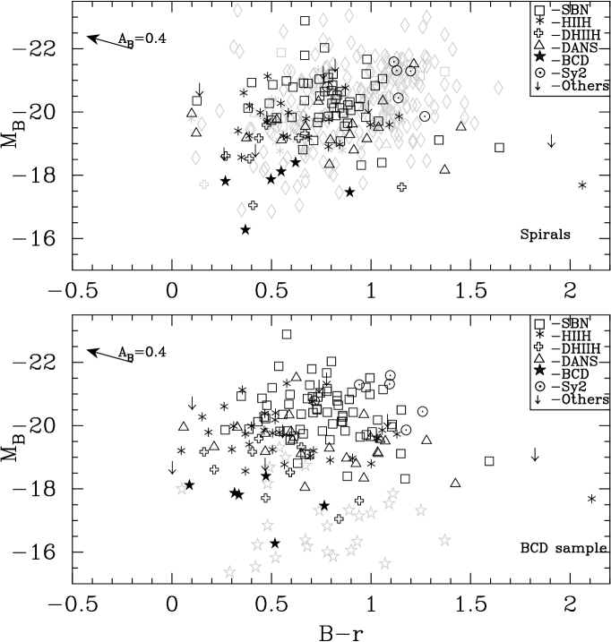
Figure 7: Colour-magnitude diagram of the UCM survey galaxies compared with other galaxies in the Nearby Universe (drawn lightened as diamonds -spirals- and five-points stars -BCD’s-). In the top panel we have used isophote 25 colours while in the second panel we have represented total colours (extracted from the $2\cdot r_{Kron}$ aperture). All absolute magnitudes are integrated total magnitudes. Typical error is that shown in Figure 6.

5 Summary

We have presented optical photometry in the Johnson $B$ and Gunn $r$ bands of the UCM Survey, a local sample of star-forming galaxies. The optical colours of UCM galaxies have been compared with the literature. Though there is a great dispersion in our data, statistically there is a good correlation between multiband photometric, morphological and spectroscopic properties.

Optical colours for the UCM galaxies, when compared with those calculated by Fukugita et al. (Fuk95 (1995)) according to their Hubble type, seem to be slightly bluer in early-type spirals and redder in irregulars and BCD’s.

Related to the spectroscopic properties of our galaxies, the calculated colours show the reddening of the objects whose $H\alpha$ emission is associated with the nucleus of the galaxy (SBN or Sy). We have also noticed that, as expected, low metallicity objects seem to be the bluest ones.

In next papers we will study the morphological properties of the UCM sample in the Johnson $B$ band. Using bulge-disk decompositions and H$\alpha$ images we will perform synthesis models and will compare global properties of our sample with the galaxy population at high redshift.

- (1) Alonso, O., García-Dabó, E., Zamorano, J., Gallego, J., Rego, M., 1999, ApJS 122, 415
- (2) Alonso-Herrero, A., Aragón-Salamanca, A., Zamorano, J., Rego, M., 1996, MNRAS 278, 417
- (3) Balzano, V. A., 1983, ApJ, 268, 602
- (4) Burstein, D. Heiles, C., 1982, AJ 87, 1165
- (5) Doublier, V., Comte, G., Petrosian, A., Turatto, M., Surace C., 1997, A&AS 124, 405
- (6) Fitzpatrick, E. L., 1999, PASP 111, 63
- (7) Fukugita, M., Shimasaku, K., Ichikawa, T., 1995, PASP 107, 945
- (8) Gallego, J., Zamorano, J., Aragón-Salamanca, A., Rego, M., 1995, ApJ 455, L1
- (9) Gallego, J., Zamorano, J., Rego, M., Alonso, O., Vitores, A. G., 1996, A&AS 120, 323
- (10) Gallego, J., Zamorano, J., Rego, M., Alonso, O., Vitores, A. G., 1997, ApJ 475, 502
- (11) Gallego, J., 1998, in Thuan T. X., Balkowski, C., Cayette, V., Tran Tranh Van, J., eds., Dwarf Galaxies and Cosmologies. Proceedings of the XVIIIth Moriond astrophysics meeting, Editions Frontieres, Gif-sur-Yvette, France
- (12) Gallego, J., 1999, Ap&SS, Proceedings of the III scientific meeting of the Spanish Astronomical Society (SEA), eds: Gorgas & Zamorano (in press)
- (13) Gil de Paz, A., Aragón-Salamanca, A., Gallego, J., Alonso-Herrero, A., Zamorano, J., Kauffmann, G., 1999, MNRAS (accepted)
- (14) Guzmán, R., Gallego, J., Koo, D. C., Phillips, A. C., Lowenthal, J. D., Faber, S. M.,Illingworth, G. D., Vogt, N. P., 1997, ApJ, 489, 559
- (15) Kron, R. G., 1980, ApJS 43, 305.
- (16) Landolt A. U. 1992, AJ, 104, 340
- (17) Madau, P., 1999, Physica Scripta, Proceedings of the Nobel Symposium, Particle Physics and the Universe (Enkoping, Sweden, August, 1998), astro-ph/9902228
- (18) Salzer, J. J., MacAlpine, G. M., Boroson, T. A., 1989, ApJS, 70, 479
- (19) Stetson, P., 1990, PASP, 102, 932
- (20) Vitores, A. G., Zamorano, J., Rego, M., Alonso, O., Gallego, J., 1996a, A&AS 118, 7
- (21) Vitores, A. G., Zamorano, J., Rego, M., Gallego, J., Alonso, O., 1996b, A&AS 120, 385
- (22) Zamorano, J., Rego, M., Gallego, J., Vitores, A. G., Gonzalez-Riestra, R., Rodriguez-Caderot, G., 1994, ApJS 95, 387
- (23) Zamorano, J., Gallego, J., Rego, M., Vitores, A. G., Alonso, O., 1996, ApJS 105, 343