Bayesian ‘Hyper-Parameters’ Approach to Joint Estimation: The Hubble Constant from CMB Measurements

Abstract

Recently several studies have jointly analysed data from different cosmological probes with the motivation of estimating cosmological parameters. Here we generalise this procedure to take into account the relative weights of various probes. This is done by including in the joint $\chi^{2}$ function a set of ‘Hyper-Parameters’, which are dealt with using Bayesian considerations. The resulting algorithm (in the case of uniform priors on the log of the Hyper-Parameters) is very simple: instead of minimising $\sum\chi_{j}^{2}$ (where $\chi_{j}^{2}$ is per data set $j$) we propose to minimise $\sum N_{j}\ln(\chi_{j}^{2})$ (where $N_{j}$ is the number of data points per data set $j$). We illustrate the method by estimating the Hubble constant $H_{0}$ from different sets of recent CMB experiments (including Saskatoon, Python V, MSAM1, TOCO and Boomerang).

1 Introduction

Several groups (e.g. Eisenstein et al. 1999, Gawiser & Silk 1998, Bridle et al. 1999, Bahcall et al. 1999, Bond & Jaffe 1998, Lineweaver 1998) have recently estimated cosmological parameters by joint analysis of data sets (e.g. CMB, SNe Ia, redshift surveys, cluster abundance and peculiar velocities).

A complication that arises in combining data sets is that there is freedom in assigning the relative weights of different measurements. Some approaches to this problem have been suggested in the astronomical literature (e.g. Godwin & Lynden-Bell 1987; Press 1996). Here we propose a Bayesian approach utilizing ‘Hyper Parameters’ (hereafter HPs).

Assume that we have 2 independent data sets, $D_{A}$ and $D_{B}$ (with $N_{A}$ and $N_{B}$ data points respectively) and that we wish to determine a vector of free parameters ${{\bf w}}$ (such as the density parameter $\Omega_{\rm{m}}$, the Hubble constant $H_{0}$ etc.). This is commonly done by minimising

$$\chi^{2}_{\rm joint}=\chi^{2}_{A}\;+\;\chi^{2}_{B}\;,$$ (1)

(or maximizing the sum of log likelihood functions). Such procedures assume that the quoted observational random errors can be trusted, and that the two (or more) $\chi^{2}$s have equal weights. However, when combining ‘apples and oranges’ one may wish to allow freedom in the relative weights. One possible approach is to generalise Eq. 1 to be

$$\chi^{2}_{\rm joint}=\alpha\chi^{2}_{A}\;+\beta\;\chi^{2}_{B}\;,$$ (2)

where $\alpha$ and $\beta$ are ‘Lagrange multipliers’, or ‘Hyper-Parameters’, which are to be evaluated in a Bayesian way. There are a number of ways to interpret the meaning of the HPs. A simple example of the HPs is the case that

$$\chi^{2}_{A}=\sum{\frac{1}{\sigma_{i}^{2}}}[x_{{\rm obs},i}-x_{{\rm pred},i}({\bf w})]^{2}\;,$$ (3)

where the sum is over $N_{A}$ measurements and corresponding predictions and errors $\sigma_{i}$. Hence by multiplying $\chi^{2}$ by $\alpha$ each error effectively becomes ${\alpha}^{-1/2}\sigma_{i}$. But even if the measurement errors are accurate, the HPs are useful in assessing the relative weight of different experiments. It is not uncommon that astronomers discard measurements (i.e. by assigning $\alpha=0$) in an ad-hoc way. The procedure we propose gives an objective diagnostic as to which measurements are problematic and deserve further understanding of systematic or random errors.

We show below that if the prior probabilities for $\ln(\alpha)$ and $\ln(\beta)$ are uniform then one should consider the quantity

$$-2\;\ln P({\bf w}|D_{A},D_{B})=N_{A}\ln(\chi_{A}^{2})+N_{B}\ln(\chi_{B}^{2})$$ (4)

instead of Eq. 1. It is as easy to calculate this statistic as the standard $\chi^{2}$. The effective HPs can then be identified as $\alpha_{\rm eff}=\frac{N_{A}}{\chi_{A}^{2}}$ and $\beta_{\rm eff}=\frac{N_{B}}{\chi_{B}^{2}}$, where $\chi^{2}_{A}$ and $\chi^{2}_{B}$ are computed at the values of the parameters ${\bf w}$ that minimise eq. 4. The derivation and interpretation of these results are given in Section 2. In Section 3 we apply the method to a set of CMB experiments and estimate the best fit Hubble constant. Extensions of the methods are discussed in Section 4.

2 ‘Hyper-parameters’

How do we eliminate the unknown HPs $\alpha$ and $\beta$ ? We follow here the Bayesian formalism given in Gull (1989), MacKay (1994) and Bishop (1995). The formalism in these references was given in the context of Maximum Entropy and Artificial Neural Networks.

By marginalisation over $\alpha$ and $\beta$ we can write the probability for the parameters ${\bf w}$ given the data:

$$P({\bf w}|D_{A},D_{B})=\int\int P({\bf w},\alpha,\beta|D_{A},D_{B})\;d\alpha\;d\beta\;.$$ (5)

Using Bayes’ theorem we can write the following relations:

$$P({\bf w},\alpha,\beta|D_{A},D_{B})=\frac{P(D_{A},D_{B}|{\bf w},\alpha,\beta)\;P({\bf w},\alpha,\beta)}{P(D_{A},D_{B})}\;,$$ (6)

and

$$P({\bf w},\alpha,\beta)=P({\bf w}|\alpha,\beta)\;P(\alpha,\beta)\;.$$ (7)

We now make the following assumptions:

$$P(D_{A},D_{B}|{\bf w},\alpha,\beta)=P(D_{A}|{\bf w},\alpha)\;P(D_{B}|{\bf w},\beta)\;,$$ (8)

$$P({\bf w}|\alpha,\beta)=const.\;,$$ (9)

$$P(\alpha,\beta)=P(\alpha)\;P(\beta)\;.$$ (10)

With the choice of ‘non-informative’ uniform priors in the log, $P(\ln\alpha)=P(\ln\beta)=1$ (Jeffreys 1939) we get $P(\alpha)=1/\alpha$ and $P(\beta)=1/\beta$. Note that the integral over priors of this kind diverges (such a prior is called ‘improper’, see Bishop 1995). These are very conservative prior, essentially stating that we are ignorant about the scale of measurements and errors. The other extreme is obviously $P(\alpha)=\delta(\alpha-1)$, i.e. when the measurements and errors are taken faithfully. One can try other forms (see below), but it is likely that these 2 extreme forms reasonably bracket the probability space. Hence:

$$P({\bf w}|D_{A},D_{B})={1\over P(D_{A},D_{B})}\;P(D_{A}|{\bf w})\;P(D_{B}|{\bf w}),$$ (11)

where

$$P(D_{A}|{\bf w})\equiv\int P(D_{A}|{\bf w},\alpha)\alpha^{-1}d\alpha\;,$$ (12)

and

$$P(D_{B}|{\bf w})\equiv\int P(D_{B}|{\bf w},\beta)\beta^{-1}d\beta\;.$$ (13)

It is common to have a likelihood function of the form of a Gaussian in $N_{A}$ dimensions:

$$P_{G}(D_{A}|{\bf w})\;\propto\;\exp[-\chi_{A}^{2}/2]\;,$$ (14)

where we assume for simplicity that the normalization constant is independent of the parameters ${\bf w}$ (this is indeed the case in our application for the CMB measurements in the next Section).

We generalise this form to incorporate $\alpha$ as follows:

$$P(D_{A}|{\bf w},\alpha)\;\propto\;\alpha^{N_{A}/2}\;\exp(-{\alpha\over 2}\chi_{A}^{2})\;.$$ (15)

The integral of Eq. 12 then gives

$$P(D_{A}|{\bf w})\propto{(\chi_{A})}^{-N_{A}}\;,$$ (16)

and similarly for Eq. 13. We note that it is the specific choice of prior for $P(\alpha)=1/\alpha$ that has led to a change from a Gaussian distribution (Eq. 14 ) to a power-law (Eq. 16).

Eq. 11 can then be written (ignoring constants) as

$$-2\;\ln P({\bf w}|D_{A},D_{B})\;=N_{A}\ln(\chi_{A}^{2})\;+\;N_{B}\ln(\chi_{B}^{2})\;.$$ (17)

To find the best fit parameters ${\bf w}$ requires us to minimise the above probability in the ${\bf w}$ space. Eq. 17 generalises a similar equation derived by Cash (1979). Cash used a very different set of arguments based on maximum likelihood and he assumed that the error per group of data is the same (in this special case the original quoted errors drop out in the minimisation). We emphasize that our Bayesian framework is more general and ‘principled’, and therefore we can derive alternative equations by assuming different priors.

Since $\alpha$ and $\beta$ have been eliminated from the analysis by marginalisation they do not have particular values that can be quoted. Rather, each value of $\alpha$ and $\beta$ has been considered, and weighted according to the probability of the data given the model. However, it may be useful to know which values of $\alpha$ and $\beta$ were given the most weight. This can be estimated by finding the values of $\alpha$ and $\beta$ at which eq 15 peaks:

$$\alpha_{\rm{eff}}=\frac{N_{A}}{\chi_{A}^{2}}\;,$$ (18)

and similarly

$$\beta_{\rm{eff}}=\frac{N_{B}}{\chi_{B}^{2}}\;,$$ (19)

both evaluated at the joint peak.

We note that if we substitute these effective $\alpha$ and $\beta$ in Eq. 2 we obtain $\chi^{2}_{joint}=N_{A}+N_{B}$, i.e. a reduced $\chi^{2}$ of unity (for the case when the number of degrees of freedom is dominated by the number of data points).

There is of course freedom in choosing the prior. For example, if we take $P(\alpha)=1$ (instead of Jeffreys’ prior $P(\alpha)=1/\alpha$) we find that the function to be minimised is $(N_{A}+2)\ln(\chi^{2}_{A})$, instead of $N_{A}\ln(\chi^{2}_{A})$. Thus these two priors give very similar results for large $N_{A}$. Numerous other priors are possible (e.g. a top-hat centred on a plausible value), but at the expense of more free HPs (e.g. the width of the top-hat).

3 Application to CMB data

We illustrate the effect of using HPs by application to measurements of the angular power spectrum of the cosmic microwave background (CMB). Numerous groups have now used CMB data to estimate cosmological parameters (see Rocha 1999 for a review). The most common method is the flat bandpower method (Bond 1995a; Bond 1995b) in which the difference between observed and predicted flat bandpowers are compared using the $\chi^{2}$ statistic (Eq. 3). There is a question as to whether one should use all measurements from all groups of observers, independent of whether a given data set is consistent with the other data. Dodelson and Knox (1999) do address this issue by assigning a calibration coefficient to each data point, the values of which are optimised for each cosmological model investigated. The HPs method offers a Bayesian alternative to ad-hoc selection of data sets or the problems associated with using incompatible data sets and a conventional approach.

There are clearly a large number of possible combinations of CMB data sets that could be investigated. For the purpose of illustration we divide a selection of the current CMB power spectrum estimates into six subsets. The subsets are (i) Saskatoon (Netterfield et al. 1997, including the five per cent calibration error; Leitch, private communication), (ii) Python V (Coble et al. 1999), (iii) MSAM1 (Wilson et al 1999), (iv) TOCO (Torbet et al. 1999, Miller et al. 1999), (v) BOOMERANG/NA (Mauskopf et al. 1999, assuming Gaussian window functions which fall by a factor of $1/e$ at $\ell_{\rm{min}}$ and $\ell_{\rm{max}}$ as specified in the paper) and (vi) we group all of the remaining data into the fifth subset and refer to it as ‘Other’. This subset contains COBE, Tenerife, South Pole, ARGO, MAX, QMAP, OVRO and CAT (see Hancock et al. 1998, Webster et al. 1998 and Efstathiou et al. 1999 for more details). These data are plotted in Fig. 1.

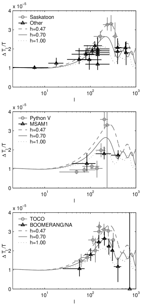
Figure 1: The CMB data used, shown in three panels for clarity. Theoretical CMB power spectra are shown for $h=0.47$, $h=0.70$ and $h=1.00$ (other parameters are fixed at the values given in the text).

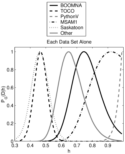
Figure 2: The probability of the Hubble constant $h$ as a function of $h$ from different subsets of CMB data (as indicated in the legend) resulting from a conventional $\chi^{2}$ analysis.

Data	$N_{j}$	Best $h$	$\chi^{2}_{j}$
BOOMERANG/NA	7	$0.75$	1.5
TOCO	9	$0.47$	10.5
MSAM1	3	$0.92$	2.1
PythonV	7	$1.00$	48.3
Saskatoon	5	$0.46$	0.5
Other	16	$0.65$	16.3

Table 1: Conventional $\chi^{2}$ analysis using each data subset alone. For each data subset the number of data points, $N_{j}$, the best fit value of $h$ and the $\chi^{2}$ value at this point is shown. The full likelihood distributions in $h$ are shown in Figure 2.

In addition, for simplicity we restrict ourselves to a very limited set of cosmological models. We assume CMB fluctuations arise from adiabatic initial conditions with cold dark matter and negligible tensor component, and that $\Omega_{\rm{m}}=0.3$, $\Omega_{\Lambda}=1-\Omega_{\rm{m}}=0.7$, $n=1$, $Q_{\rm{rms-ps}}=18\mu$K and $\Omega_{b}h^{2}=0.019$. We then investigate the constraints on the remaining parameter, the dimensionless Hubble constant, $h=H_{0}/(100$ $\rm{km}\rm{s}^{-1}\rm{Mpc}^{-1}$$)$. Theoretical power spectra for three different values of $h$ are shown in Fig. 1: increasing $h$ decreases the height of the first acoustic peak, and makes few other significant changes for the purpose of our analysis. The range in $h$ investigated here ($0.3<h<1.0$) takes the peak height from above the Saskatoon upper error bars down to the MSAM1 points.

To aid qualitative understanding of the analysis that follows, it is helpful to first calculate the value of $h$ preferred by each data subset. The results are plotted in Fig. 2 and shown in Table 1. As expected from the range of first acoustic peak heights preferred by the data, the $h$ values also vary considerably. The BOOMERANG/NA data alone prefers an intermediate value of $h$, as does the ‘Other’ data. TOCO and Saskatoon both agree on a relatively high first acoustic peak and so on a low $h$. The MSAM1 points are quite low and thus fit a high value of $h$, and the PythonV points also prefer a high value of $h$, although the $\chi^{2}$ value is very high, indicating a bad fit to the model.

Clearly there are a large number of possible groupings of the data subsets. We show here the results from just five groupings, which are a fair sample and also highlight some of the properties of HPs. Firstly we consider the case of two relatively discrepant data sets, Saskatoon and BOOMERANG/NA; the $h$ values that they prefer do not overlap significantly. Combining their $\chi^{2}$ values for each $h$ in the conventional manner (Eq. 1) yields the likelihood function plotted with the dotted line in Fig. 3 (Top). An intermediate value of $h$ is preferred, and in fact the best fitting $h$ values for each data set alone are essentially ruled out. In contrast, when HPs are used, i.e. the $\chi^{2}$ values are combined using Eq. 17, the dotted line in Fig. 3 (Bottom) is obtained. There are two peaks in the probability distribution corresponding to the two different values of $h$ preferred by each data set alone. This is perhaps closer to what we would actually believe given just these two data subsets.

Next we consider the effect of adding in a data subset that agrees strongly with one of the above two data subsets. That is, we consider TOCO with Saskatoon and BOOMERANG/NA. The probability distribution calculated using HPs now loses its second peak, retaining the one that agrees with TOCO and Saskatoon. The theoretical CMB power spectrum for the preferred value of $h=0.47$ is shown in Fig. 1.

On combining two data sets that do agree well, BOOMERANG/NA and ‘Other’, there is little difference between the conventional and HP analyses, although the error bar on $h$ is slightly decreased when using HPs.

Adding in a data subset that has a poor $\chi^{2}$ (given the range of models considered), PythonV, makes a large difference to the conventional analysis but only a very small difference to the HP analysis. This can also be seen from the effective HP value at the best fit $h$, calculated from Eq. 18, which is much less than unity for the PythonV data, indicating that it has been down weighted.

Finally we use all of the data subsets, obtaining the solid lines in Fig. 3. It turns out that the best fitting value of $h$ is similar in both the conventional and HP analyses, but the error bars are significantly wider in the HP analysis, which corresponds better to what we would naturally believe.

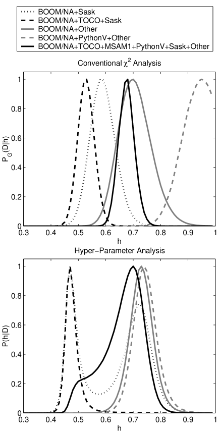
Figure 3: The probability of the Hubble constant $h$ as a function of $h$ from different subsets of CMB data (as indicated in the legend) resulting (Top figure) from a conventional $\chi^{2}$ analysis and (Bottom figure) the Hyper-Parameter analysis, in which $P(h|D_{A},D_{B},\ldots)=\exp[-{\frac{1}{2}}\sum N_{j}\ln(\chi^{2}_{j})]$.

Data	$N_{j}$	Best $h$	$\chi^{2}_{j}$
BOOM/NA+Sask	12	$0.58$	11.3
BOOM/NA+TOCO+Sask	21	$0.53$	25.6
BOOM/NA+Other	23	$0.70$	18.6
BOOM/NA+PythonV+Other	30	$0.95$	81.2
All data	47	$0.68$	152.6

Table 2: Conventional $\chi^{2}$ analysis. Best fit values of $h$ and $\chi^{2}$ values at this best fit point, which can be compared to the total number of data points, $N_{j}$.

Data	$N_{j}$	Best $h$	$\chi^{2}_{j}$			Effective		HP
BOOMERANG/NA	7	0.47	18	.	5	0	.	4
Saskatoon	5		0	.	5	10	.	2
BOOMERANG/NA	7	0.47	18	.	5	0	.	4
TOCO	9		10	.	5	0	.	9
Saskatoon	5		0	.	5	10	.	2
BOOMERANG/NA	7	0.73	1	.	5	4	.	5
Other	16		17	.	4	0	.	9
BOOMERANG/NA	7	0.74	1	.	5	4	.	5
PythonV	7		73	.	1	0	.	1
Other	16		17	.	6	0	.	9
BOOMERANG/NA	7	0.70	1	.	8	3	.	9
TOCO	9		34	.	9	0	.	3
MSAM1	3		5	.	4	0	.	6
Python V	7		79	.	6	0	.	1
Saskatoon	5		14	.	9	0	.	3
Other	16		16	.	8	1	.	0

Table 3: The five different combinations used in the Hyper-Parameter analysis. In each case a separate Hyper-Parameter was given to each data subset, the number of data points in each data subset, $N_{j}$, is shown. The best fitting value of $h$, the $\chi^{2}$ value for each data subset for this best fitting $h$ and the effective HP ($N_{j}/\chi^{2}_{j}$) at this $h$ is calculated.

4 Discussion

We have presented a formalism for analyzing a set of different measurements. By using a Bayesian analysis, and by using a ‘non-informative’ prior for the ‘Hyper-Parameters’, we find that for $M$ data sets one should minimise

$$-2\;\ln P({\bf w}|{\rm data})=\sum_{j=1}^{M}N_{j}\ln(\chi_{j}^{2}),$$ (20)

where $N_{j}$ is the number of measurements in data set $j=1,...,M$. It is as easy to calculate this statistic as the standard $\chi^{2}$. The corresponding HPs $\alpha_{{\rm eff},j}=N_{j}/\chi^{2}_{j}$ provide useful diagnostics on the reliability of different data sets. We emphasize that a low HP assigned to an experiment does not necessarily mean that the experiment is ‘bad’, but rather it calls attention to look for systematic effects or better modelleing.

We have applied the HP analysis to a set of various CMB measurements and estimated the Hubble constant $H_{0}$ (for a fixed flat CDM $\Omega_{\rm m}=1-\lambda=0.3$ model). While the standard $\chi^{2}$ approach gives a wide range for $H_{0}$, the Hyper-Parameter analysis suggests two distinct values of $H_{0}$, $\sim 50$ and $\sim 70$ km/sec/Mpc. It remains to be understood why the ensemble of CMB experiments tends to give two competing values (quite common in the history of the Hubble constant !). It would be most interesting to see how these values change when combined with other cosmological probes (and their corresponding HPs).

In estimating $H_{0}$ we have assumed that the other cosmological parameters (like $\Omega_{\rm{m}}$ and $\Omega_{\Lambda}$) were known and, consequently, such an estimate is conditional on the assumed values of these parameters. This is not strictly necessary, actually, since we may obtain a more general estimation of $H_{0}$ by marginalising over $\Omega_{\rm{m}}$, $\lambda$, and the other cosmological parameters, in a way similar to what we have done with the HPs. One may also generalise the above method for more specific applications. Two aspects which can be modified according to specific problems are the priors $P(\alpha_{j})$ and the probability functions $P(D_{j}|{\bf w})$. We shall discuss elsewhere these extensions in application to various cosmological probes.

Acknowledgments: We thank G. Rocha for her contribution to the data analysis, and A. Dekel and I. Zehavi for helpful discussions. SLB acknowledges the receipt of a PPARC studentship. OL thanks the IAG (São Paulo) for hospitality. LSJ thanks FAPESP, CNPq and PRONEX/FINEP for the support to his work.

References

- [1] Bahcall, N.A., Ostriker, J.P., Perlmutter, S., Steinhardt, P.J., 1999, Science, 284, 148
- [2] Bishop, C.M., 1995, Neural Networks for Pattern Recognition, Oxford University Press, Oxford
- [3] Bond, J. R., 1995a, Cosmology and Large Scale Structure, Proc. Les Houches School, Session LX, August 1993. ed Schaeffer, R. Elsevier Science Publishers, Netherlands
- [4] Bond, J. R., 1995b, Astrophys. Lett. and Comm., 32, 63
- [5] Bond, J. R. & Jaffe, A. H., 1998, Philosophical Transactions of the Royal Society of London A, 1998. Discussion Meeting on Large Scale Structure in the Universe, Royal Society, London, March 1998.
- [6] Bridle, S.L., Eke, V.R., Lahav, O., Lasenby, A.N., Hobson, M.P., Cole, S., Frenk, C.S., Henry, J.P., 1999, MNRAS, in press (astro-ph/9903472)
- [7] Cash, W., 1979, ApJ, 228, 939
- [8] Coble, K. et al., 1999, preprint (astro-ph/9902195)
- [9] Dodelson, S., Knox, L., submitted to PRL, 1999 (astro-ph/9909454)
- [10] Efstathiou G., Bridle S. L., Lasenby A. N., Hobson M. P., Ellis R. S. 1999, MNRAS, 303, L47
- [11] Eisenstein, D.J., Hu, W., Tegmark, M., 1999, ApJ, 518, 2
- [12] Gawiser E., Silk J., 1998, Science, 280, 1405
- [13] Godwin, P., Lynden-Bell, D. 1987, MNRAS, 229, 7
- [14] Gull, S.F., 1989, in Maximum Entropy and Bayesian Methods, Cambridge 1988, ed. J. Skilling, p. 53, Dordrecht: Kluwer
- [15] Hancock, S., Rocha, G., Lasenby, A. N., & Gutierrez, C. M. 1998, MNRAS, 294, L1
- [16] Jefferys, H., 1939, Theory of Probability, Oxford University Press (1983 edition)
- [17] Lineweaver, C. H. 1998, ApJ, 505, L69
- [18] MacKay, D., 1994, in Maximum Entropy and Bayesian Methods, Santa Barbara 1993, ed. G. Heidbreder, Dordrecht: Kluwer
- [19] Mauskopf, P. et al. 1999, preprint (astro-ph/9911444)
- [20] Miller, A., et al. 1999, submitted to ApJL (astro-ph/9906421)
- [21] Netterfield, C. B., Devlin, M. J., Jarolik, N., Page, L., Wollack, E. J., 1997, ApJ 474, 47
- [22] Press, W.H., 1996, in Unsolved Problems in Astrophysics, Proceedings of Conference in Honor of John Bahcall, ed. J.P. Ostriker, Princeton: Princeton University Press (astro-ph/9604126)
- [23] Rocha, G. 1999, Invited review to appear in the proceedings of the Early Universe and Dark Matter Conference, DARK98, Heidelberg, 1998 (astro-ph/9907312)
- [24] Torbet, E., et al. 1999, ApJL, 521, L79
- [25] Webster, M., Bridle, S.L., Hobson, M.P., Lasenby, A.N., Lahav, O., & Rocha, G. 1998, ApJ Lett, 509, L65
- [26] Wilson, G., et al. 1999, preprint (astro-ph/9902047)