A method for detecting gravitational waves coincident with gamma ray bursts

Abstract

The mechanism for gamma ray bursters and the detection of gravitational waves (GWs) are two outstanding problems facing modern physics. Many models of gamma ray bursters predict copious GW emission, so the assumption of an association between GWs and GRBs may be testable with existing bar GW detector data. We consider Weber bar data streams in the vicinity of known GRB times and present calculations of the expected signal after co-addition of 1000 GW/GRBs that have been shifted to a common zero time. Our calculations are based on assumptions concerning the GW spectrum and the redshift distribution of GW/GRB sources which are consistent with current GW/GRB models. We discuss further possibilities of GW detection associated with GRBs in light of future bar detector improvements and suggest that co-addition of data from several improved bar detectors may result in detection of GWs (if the GW/GRB assumption is correct) on a time scale comparable with the LIGO projects.

1 Introduction

The attempts to detect gravitational radiation began with the work of Weber (1960). The existence of gravitational waves has been verified indirectly by observations of the decay in orbital period of the pulsar PSR 1913+16 (Hulse & Taylor 1975), for which the 1993 Nobel Prize in Physics was awarded. However, direct detection continues to prove elusive even though some authors believed it to be possible before the turn of the century (eg. Thorne 1992). Detection remains difficult due to the nature of the coupling between energy and spacetime. Although a large amount of energy might be stored in gravitational waves (GWs), the corresponding amplitude of the waves, measured in dimensionless strain, $h$, is exceedingly small due to the very small magnitude of the proportionality constant in Einstein’s equations: a large stress-energy produces a very small metric perturbation.

The most sensitive detectors currently in operation are of the Weber bar variety. The main detectors are maintained at the University of Western Australia (eg. Heng et al. 1996), Louisiana State University (eg. Mauceli et al. 1996), the University of Rome (eg. Astone et al. 1993), Legnaro National Laboratories (eg. Cerdonio et al. 1995) and Laboratori Nazionali di Frascati (eg. Coccia et al. 1995). These detectors have a very low bandwidth as they rely on detection of the resonance in the bar (or sphere) after a burst of GWs. Near the resonance frequency, bar detectors are capable of reaching sensitivities of $\sim 10^{-19}$–$10^{-18}$ (eg. Tobar et al. 1995) and future sensitivities are expected to reach $\sim 10^{-20}$ (eg. Tobar et al. 1998). Spurious, non-thermal excitations of resonant bars typically number $\sim 40$ per day (Heng et al. 1996). Thus, detection of a real, individual GW burst will require coincidence with detections by other instruments around the world. No convincing coincidences have been recorded to date.

The LIGO/VIRGO network is expected to detect gravitational waves (Finn & Chernoff 1993; Cutler & Flanagan 1994; Thorne 1994; Flanagan & Hughes 1998), if not in the initial stages when the sensitivity of LIGO is $\sim 10^{-21}$, then in the advanced stage when it is $\sim 3\times 10^{-23}$. This will mark the beginning of GW astronomy, promising views of neutron star (NS) and black hole (BH) coalescence and collisions. It will also yield detailed information about the dynamics of pulsar systems and may even allow us to study inflation and the Big Bang itself more directly and in much more detail than other astrophysical techniques allow.

Another problem that has confronted science for decades has been the origin of gamma ray bursts (GRBs). Many theories for the emission of GRBs centre on a mechanism involving large mass quadrupole moments. Hence a wide variety of GRB models predict large GW luminosities. For example, NS mergers are good candidates for GRBs (eg. Kochanek & Piran 1993; Dokuchaev, Eroshenko & Ozernoy 1998) and are expected to result in $\sim 10^{52}{\rm~{}ergs}$ in GWs (Centrella & McMillan 1993; Ruffert & Janka 1998). Such energies result in detectable GW signals if the NSs are in the Galaxy but if the source is cosmological both modern bar detectors and the advanced LIGO system cannot detect such events.

It is this expected association between the two phenomena that has prompted the present investigation. With the expectation that GW bursts are temporally correlated with GRBs, we may co-add existing GW data surrounding measured GRB events. This would result in a composite GW data stream with all GRB events shifted to a common ‘GRB time’. We explore this idea below and present a method offering up to a factor of $\sim 30$ increase in signal-to-noise ratio (SNR) with the co-addition of 1000 existing GW data streams surrounding measured GRB times. Throughout the work, we assume that all the measured GRBs are associated with GW emission.

In this article we calculate the expected signal from a typical bar detector assuming that the bar is noiseless. Our aim is to show directly, with some generality, whether available data from GRB and GW detectors can be used to detect GWs before the first LIGO/VIRGO detection. Such a detection would also be confirmation of an association between the GRB mechanism and GW emission.

Our calculations are based on various assumptions concerning source distribution in spacetime, the nature of the source and the corresponding GW emission, all in line with current models. We compare our calculations with the noise floor of the bar and decide on the viability of such a method for detection using bar detectors. We also discuss the viability of detection by the LIGO system.

The paper is organized as follows. In Section 2 we provide the formalism for our calculations, discussing the assumptions concerning the GW source and detector. Various models are considered in Section 3 that are consistent with the assumption that GRBs are associated with GW emission. From this discussion we extract features such as the redshift distribution of sources and the spectrum of the source. In Section 4 we compute the signal seen at the detector for a single GW/GRB. We also simulate the co-addition of bar data with the assumption of a common temporal zero point and we discuss the results for the various models in Section 4. In Section 5 we discuss the relevance of our result for the LIGO/VIRGO experiments and provide our conclusions.

2 Formalism

Our aim is to calculate the signal seen at the output of a GW bar detector, with a single resonance band, due to a single GW burst. However, we keep in mind that we ultimately wish to simulate the composite effect due to many bursts (shifted to a common burst time); we wish to obtain a Monte Carlo estimate of the signal at the bar output after data processing. We therefore assume that there exists a distribution of GW/GRB sources in spacetime according to the normalized redshift distribution, $\phi(z)dz$. That is, we require that $\int\phi(z)dz=1$. To calculate the effect on the detector we need to find the GW spectrum at the bar due to a source under this distribution. Therefore, let us assume that the frequency of GWs at the source is described by the spectral profile $f(\nu)d\nu$. Again, $\int f(\nu)d\nu=1$. Also, since we are considering the spectrum of the source, we may calibrate the GW flux scale by assuming that the average total energy emitted in GWs by the source is $F$. We explain our reasoning below.

2.1 GW emission and propagation

Our first assumption is of a distribution of mean total GW fluxes at the detector. The analysis is based on the assumption that GRBs are associated with GW emission. We further assume that the observed luminosity distribution of GWs in the detector frame follows that of GRBs. This assumption is valid only if the mechanism for gamma ray and GW emission is closely physically related. We make this assumption on the basis that our results may then be used as constraints for such a subset of GW/GRB theories and because of the lack of other reasonable models for the luminosity distribution of GW sources under the GW/GRB assumption. The knowledge of whether this relationship holds in reality would be invaluable for theories of gamma ray bursters.

It is common to define the Earth frame luminosity distribution of GRBs in terms of the number of bursts with peak gamma ray flux greater than a given peak flux, $P$, as $N_{\rm{\sc grb}}(>P)$. The fact that this distribution strays from a $-3/2$ power law at low $P$ is an indication of the cosmological origin of GRBs. This has been confirmed by several optical transient observations and redshift determinations (eg. Metzger et al. 1997; van Paradijs et al. 1997; Djorgovski et al. 1998; Kulkarni et al. 1998). $P$ is usually defined in terms of a given Earth frame energy band and the integration time over which the flux was allowed to accumulate. We use the distribution measured by the BATSE instrument – supplied in the BATSE 4Br catalogue (Paciesas et al. 1999) – choosing the $50$–$300{\rm~{}keV}$ energy band and the $64{\rm~{}ms}$ integration time. In our calculations, it is convenient to find the cumulative distribution of total GW fluxes. We define this as

$$n_{\rm{\sc gw}}[<P(S^{\prime})]=1-\frac{N_{\rm{\sc grb}}(>P)}{N_{\rm{\sc grb}}}$$ (1)

where $N_{\rm{\sc grb}}$ is the total number of GRBs in the distribution and $P(S^{\prime})$ is defined as

$$P(S^{\prime})=\frac{\bar{P}}{\bar{S^{\prime}}}\,S^{\prime}\,.$$ (2)

Here, $\bar{P}$ is the average value of the peak flux in gamma rays and $\bar{S^{\prime}}$ is the mean flux in GWs at the detector.

$\bar{P}$ is easily computed from the data in the BATSE 4Br catalogue. We obtain $\bar{S^{\prime}}$ by evolving $F$ with cosmology from the source to the detector. This is particularly simple in the case of a flat universe in which the cosmological constant is vanishingly small (Misner, Thorne & Wheeler 1973, p. 783),

$$\bar{S^{\prime}}(F,z_{\rm m})=\frac{F}{4\pi(1+z_{\rm m})^{2}{\cal R}(z_{\rm m})^{2}}$$ (3)

where the distance, ${\cal R}(z_{\rm m})$ is defined by

$${\cal R}(z_{\rm m})=\frac{2+2z_{\rm m}-2\sqrt{1+z_{\rm m}}}{H_{0}(1+z_{\rm m})}\,.$$ (4)

Here, $H_{0}$ is the Hubble constant and $z_{\rm m}$ is the mean of the redshift distribution ($c$ has been set to unity in Eqs. 3 and 4). Throughout this work, we use $H_{0}=75{\rm~{}kms^{-1}Mpc^{-1}}$. So, by choosing a model of the source, we can estimate $F$ and normalize the flux scale of $n_{\rm{\sc gw}}(<P(S^{\prime}))$ to the units of GW flux using Eq. 2.

Since we are interested in the frequency space at the detector, we may convert the assumed redshift distribution, $\phi(z)dz$, to a GW frequency distribution at the detector, $\phi_{\nu}^{\prime}(\nu^{\prime})d\nu^{\prime}$, using the simple transformation, $1+z=\nu/\nu^{\prime}$. This leads directly to

$$\phi_{\nu}^{\prime}(\nu^{\prime})=(\nu^{\prime})^{-2}\phi\left(\frac{\nu}{\nu^{\prime}}-1\right)$$ (5)

provided that we have a value for $\nu$, the frequency of GW at the source at redshift $z$. We interpret $\nu$ as being the mean frequency at the source under the distribution $f(\nu)d\nu$. It is also convenient to define the cumulative frequency distribution at the detector,

$$\Phi_{\nu}^{\prime}(\nu^{\prime})=\int_{0}^{\nu^{\prime}}\phi_{\nu}^{\prime}(\xi)d\xi\,.$$ (6)

Since we ultimately wish to co-add the signals from many GWs bursts associated with GRBs, we may choose a luminosity from $n_{\rm{\sc gw}}(<S^{\prime})$ by randomly selecting a value for $n_{\rm{\sc gw}}$ and finding the corresponding value of $S^{\prime}$. Similarly, we use Eq. 6 to find a random value for the mean GW frequency at the detector. Since we have assumed a normalized GW spectral profile of the source, $f(\nu)d\nu$, which has a mean frequency of $\bar{\nu}$, we may find the mean GW frequency at the detector given a single GW/GRB burst. That is, by specifying both the mean frequency at the source and at the detector, we have randomly selected the source redshift. Using this redshift we can find the full spectrum at the detector by multiplying our selected value for $S^{\prime}$ by the redshifted spectral profile, $f^{\prime}_{\bar{\nu}}(\nu^{\prime})d\nu^{\prime}$.

2.2 GW detection

2.2.1 General

We may now discuss the detection of such a GW burst. We assume that the GW burst bandwidth is much greater than that of the bar detector since the later is typically of the order of $\sim 0.3{\rm~{}Hz}$ (Tobar et al. 1995). The cross section for a single bar resonance in response to GWs in such a situation is given by (Paik & Wagoner 1976)

$$\Sigma_{\nu^{\prime}_{0}}=\frac{32}{15}\frac{M}{\pi}\left(\frac{G}{c}\right)\left(\frac{v}{c}\right)^{2}\left\{1+O\left[\left(\frac{R}{L}\right)^{2}\right]\right\}\,,$$ (7)

where $M$ is the mass of the bar, $v$ is the speed of sound in the bar, $R$ is the radius of the physical cross section and $L$ is the length of the bar. Eq. 7 assumes that, on the average, GW bursts are incident isotropically on the detector with random polarisations. In most bar detectors, $R\ll L$ and so the second order terms are neglected. We can then find the amplitude of vibration (in strain) that the absorption of GWs causes in the bar (Misner, Thorne & Wheeler 1973, p. 1039),

$$h=\frac{1}{L}\left(\frac{S^{\prime}\Sigma_{\nu^{\prime}_{0}}f^{\prime}_{\bar{\nu}}(\nu^{\prime})d\nu^{\prime}|_{\nu^{\prime}_{0}}}{2\pi^{2}(\nu_{0}^{\prime})^{2}M}\right)^{1/2}\,.$$ (8)

2.2.2 The Niobium bar detector at UWA

The discussion above has remained general for most cylindrical bar detectors. However, for the remainder of the analysis, we take the specific example of the Niobium bar detector at the University of Western Australia, NIOBE, since we wish to model the detection algorithms in order to estimate the signal seen at the outputs. The results will carry a factor of $\sim 5$–$10$ uncertainty and so they will remain representative of most bar detectors. In particular, we consider the simplest algorithm to analyse GW data streams, the zero order prediction (ZOP) technique. Here we summarize some main points. For details of the detection methods used for NIOBE and for descriptions of the ZOP algorithm, see Tobar et al. (1995), Dhurandhar, Blair & Costa (1996) and Heng et al. (1996).

GW data are sampled at $0.1{\rm~{}s}$ intervals and passed through an optimal low-pass filter before being decimated to $1{\rm~{}Hz}$ samples. Correction factors for the low-pass procedure are included and the results are scaled to noise temperature or strain. For an $\sim 1{\rm~{}ms}$ burst of GWs, the rise time for the amplitude of vibration in the detector is also $\sim 1{\rm~{}ms}$. However, due to the high $Q$-factor, the amplitude decays exponentially over a time scale of $\sim 200{\rm~{}s}$. The fact that the data are decimated means that the signal seen after the data are processed is essentially the time derivative of the data. That is, if we model the decay in strain amplitude by

$$h(t)=\sqrt{2}\,h\left[\exp\left(-t\frac{dt}{T_{\rm mode}}\right)-\exp\left(-t\frac{dt}{T_{\rm int}}\right)\right]$$ (9)

then we may obtain an estimate of the signal after data processing using

$$\bar{h}(t)=\sqrt{2}\,h\left|\frac{dt}{T_{\rm mode}}\exp\left(-t\frac{dt}{T_{\rm mode}}\right)\right.-$$

$$\left.\frac{dt}{T_{\rm int}}\exp\left(-t\frac{dt}{T_{\rm int}}\right)\right|\,,$$ (10)

where $t$ is a dimensionless measure of the time after the GW burst that takes into account the sampling time in the decimated data. $T_{\rm mode}$ is the ring down time for the mode of oscillation in the bar, $T_{\rm int}$ is the integration time for data samples and $dt$ is the time step for data sampling. In our case $dt=T_{\rm int}$ and $T_{\rm mode}\sim 200{\rm~{}s}$. This analysis does not take account of the noise floor of the detector which will completely swamp such a single GW burst signal. Also, we do not take account of any attenuation of the signal resulting from the low-pass filtering; we assume that the processing algorithm corrects for this.

2.3 Co-addition Simulation

We are now in a position to set up a Monte Carlo simulation to estimate the signal in Eq. 2.2.2. We must choose a model for the source so as to estimate the GW spectral profile and the mean total GW energy output per burst. The formalism above implicitly assumes that all GW bursts last for less than $\sim 1{\rm~{}s}$ and this must be reflected in the model of the GW emission. We must also assume a redshift distribution of sources. The models considered here will be discussed in Section 3. Given one of the set of models, however, we may find a value for $S^{\prime}f^{\prime}_{\bar{\nu}}(\nu^{\prime})d\nu^{\prime}|_{\nu^{\prime}_{0}}$ and use Eqs. 7 and 8 to find the signal after the data processing, Eq. 2.2.2. By using the cumulative distributions, Eqs. 1 and 6, we can build up a simulation of many bursts and find their collective effect on the detector.

Throughout this work we assume, as a worst case estimate, that GRB times are uniformly distributed over $10{\rm~{}s}$ after the emission of the corresponding GW bursts (Kochanek & Piran 1993). However, we provide a scaling of our results for a range of time lags in Section 4 (see Fig. 2) since a less conservative view would put most GW bursts only $\sim 1{\rm~{}s}$ before the GRB. The ‘GRB time’ may be the trigger time in the BATSE catalogue or it may be the time at which the gamma ray flux sees a significant increase over threshold. The difference between such definitions could be, at most, $\sim 10{\rm~{}s}$. This issue is complicated by the irregular and complex intensity profiles of GRBs (eg. Fishman & Meegan 1995). Here, for purposes of simulation, we assume that this problem is resolved so that all the ‘GRB times’ are aligned.

Finally, we note that the treatment above is valid only for a bar detector with a single resonance band. However, as our calculations are aimed at simulating the effect on NIOBE, which has two resonant frequencies, the plus mode at $\nu_{0+}^{\prime}\sim 713{\rm~{}Hz}$ and the minus mode at $\nu^{\prime}_{0-}\sim 694.5{\rm~{}Hz}$, we make the following adjustment to the formalism. NIOBE acts approximately as a coupled two mass oscillator. As a rough approximation, we may therefore model the detector as having two resonance bands with cross sections given by Eq. 8 centred at the relevant resonant frequencies.

3 Models

In this section we consider the parameters associated with various GW/GRB models. Most of the resulting consistent sets of parameters describe binary coalescence models as these seem to be the most likely GW/GRB source if indeed the GW/GRB assumption is correct (Kochanek & Piran 1993). The remaining sets are, therefore, more speculative and provide useful comparisons with the binary coalescence models in view of the final results in Section 4.

In order to define a specific GW/GRB model we must specify the following.

1. Burst Mechanism: Among the competing mechanisms for GRBs are NS collision and coalescence (e.g. Piran 1991; Kochanek & Piran 1993; Totani 1997; Ruffert & Janka 1998) and other more general coalescence scenarios, such as BH–NS (eg. Lee & Kluźniak 1998) and white dwarf–BH coalescences (eg. Fryer et al. 1999). These mechanisms all imply that the source space density should follow (if somewhat lagged in time) the massive star formation rate (eg. Totani 1997; Krumholz, Thorsett & Harrison 1998). Other authors prefer to assume source space densities that are similar to the quasar redshift distribution (eg. Horak, Emslie & Hartmann 1995) without venturing as to what the mechanism for GRBs might be.

2. Spectral profile, $f(\nu)d\nu$: For close binary systems, the emission of GWs leads to energy loss and in-spiral. The GW frequency therefore follows a ‘chirrup’ pattern, monotonically increasing with time. The Newtonian approximation for the in-spiral is a good one up until the few rotation periods before coalescence when post-Newtonian corrections become important. The innermost stable orbit marks the point at which GW emission begins to decrease because of the increase in the infall rate of the component stars. The innermost stable orbit occurs at an orbital separation of $r\sim 6M$ (Kidder, Will & Wiseman 1992, setting $G=c=1$) and so Cutler & Flanagan (1994) propose that the GW emission will shut off at roughly $\bar{\nu}=(6^{3/2}\pi M)^{-1}$ for $M$ the total mass of the binary system. The important parameters to obtain here are the mean frequency of GW emission at the source and the spectral profile. For a NS–NS system, the mass may lie in the range $M=(2.70\pm 0.08)M_{\sun}$ (Thorsett & Chakrabarty 1999). We therefore find that the frequency of maximum emission is $\bar{\nu}\sim 1600{\rm~{}Hz}$ and that the width of the distribution of these frequencies is $\sim 100{\rm~{}Hz}$. Assuming that the ‘chirrup’ is very steep near the coalescence and that the frequency of emission is within $\sim 500{\rm~{}Hz}$ of $\bar{\nu}$ for $\ll 1{\rm~{}s}$ (eg. Allen 1997; Allen 1999) , we may assume, as we ultimately wish to co-add signals at the detector, that the spectral profile at the source for NS–NS coalescence has a width of $\sigma\sim 500{\rm~{}Hz}$.

   The issue of the actual value of $\bar{\nu}$ is of more importance here since we are dealing with such a low bandwidth detector. However, it is a poorly known quantity due to the slow convergence of post Newtonian corrections to the estimate above. Using the results of post Newtonian calculations of the final moments of in-spiral (Finn & Chernoff 1993; Cutler & Flanagan 1994; Blanchet 1996) we find values in the range $\sim 1200$ to $\sim 1500{\rm~{}Hz}$. We also note that estimates by Kidder, Will & Wiseman (1992, 1993), Damour, Iyer & Sathyaprakash (1998) and Allen et al. (1999) suggest that $\bar{\nu}=1420,~{}2042.6{\rm~{}and~{}}1822{\rm~{}Hz}$ respectively for $M=2.8M_{\sun}$. It is therefore desirable to assume a range of frequencies for each model of binary coalescence.

   We also note that, for coalescence scenarios involving a BH, the higher mass of the BH relative to that of a NS reduces the GW frequency. It is therefore likely that GW emission from such systems will result in a low flux at the detector resonant frequency. Consequently, we do not consider such systems in our calculations.

   With regards to NS collisions, little information can be gained as to the general spectral profile of the source since this depends on the separation of the path trajectories. Therefore, we do not consider collisions in our calculations.

   Finally, assuming that the GW/GRBs are associated with the quasar redshift distribution gives no information on the distribution of frequencies at the source; the GW mechanism has not been specified. We will therefore assume a broad band emission in such an instance so as to compare with results from the NS coalescence models. We will also consider a range of mean redshifts, $z_{\rm m}$, in such models.

3. Mean total emitted GW energy, $F$: For NS coalescences, this is known to reasonable accuracy, but clearly, for our quasar model, we have no information on this parameter. Let us therefore remove $F$ from consideration in this instance by assuming that it is the same as the range we will assume for NS coalescences. Various authors suggest that $F$ lies in the range $10^{51}$–$10^{53}{\rm~{}ergs}$ (eg. Rasio & Shapiro 1992; Centrella & McMillan 1993; Oohara & Nakamura 1995; Lee & Kluźniak 1998) based on both numerical and approximate theoretical grounds. We therefore provide calculations for this order of magnitude.

4. Number of bursts, N: From the formalism in Section 2, we see that if the number of bursts is large then the sum of all $h$ for all bursts will scale approximately linearly with N. Therefore, throughout our calculations we will assume that $N=1000$ as a representative value. We compare this with the number of bursts in the BATSE 4Br catalogue, $N_{\sc batse}=1637$, and note that over $2000$ burst times have been recorded. If the co-addition of GW data were to be performed, the number of bursts available would be restricted by the fact that most bursts do not have a simple intensity profile over the BATSE integration time. That is, it may be difficult to assign a burst time to a given GRB due to the complex nature of the profile. We therefore keep $N=1000$ as an estimate of the number of useful bursts for the current purpose.

   In any co-addition of “real” data, the SNR will rise in proportion to $\sqrt{N}$ for $N$ the number of data streams to be co-added. The noise is co-added together with the signal; the signal rising in proportion to $N$ and the noise in proportion to $\sqrt{N}$. However, our co-addition of simulated data does not include the noise characteristics of the bar. If we are to compare our final results with the sensitivity of the detector for a single burst, the comparison must be between our noiseless results and $\sqrt{N}$ times the typical noise at the resonance. We make this comparison in Section 4.

We have therefore narrowed our view of models of GW/GRBs to two main sets of parameters. The first is the set associated with the assumption that GRBs are due to coalescence of binary NS systems. We shall call this the NS–NS model and take those parameters discussed above for it. We assume a star formation redshift distribution that follows that of Madau, Pozzetti & Dickinson (1998) (hereafter MPD) and compare this with that given by Pascarelle, Lanzetta & Fernández-Soto (1998) (hereafter PLFS). The later compares well with the findings of Totani (1997) that the star formation rate needs to be a factor of $5$–$10$ higher at redshifts $z\mathrel{\hbox to0.0pt{\lower 3.0pt\hbox{$\mathchar 536\relax$}\hss}\raise 2.0pt\hbox{$\mathchar 318\relax$}}2$ for the NS–NS scenario to be consistent with the BATSE data.

However, as a useful comparison, we parametrize the somewhat undefined quasar model by assuming a Gaussian redshift distribution, centred on a range of redshifts, $1.5<z_{\rm m}<3.0$ with a constant width, $\sigma=0.45$ (Horack, Emslie and Hartmann 1995). The range in $z_{\rm m}$ may be interpreted as a time lag factor (positive or negative) due to the specific (unknown) mechanism of GW/GRBs. We also include such a time lag effect in the star formation redshift distributions due to the length of time needed for complete in-spiral of close NS–NS systems. We vary this time lag in redshift space from $\sim 0.8$ to $0$ by allowing the redshift at which the star formation rate first reaches a maximum, $z_{\rm p}$, to vary. We illustrate some typical redshift distributions in Fig. 1.

Figure 1: Comparison of three typical redshift distributions. The top panel shows a MPD-like distribution and the middle panel shows a rough fit to the redshift distribution in PLFS. The bottom panel shows the quasar-like distribution used as a comparative example in our calculations. All distributions are normalized to unity.

4 Results and Discussion

For a specific model defined in the previous section, with a given mean source frame frequency, $\bar{\nu}$, and a specific redshift distribution, we obtain results typified by those shown in Fig. 2. Of note is the distribution of $h$ shown by the points. These are co-added to give a generally increasing signal, $\bar{h}(t)$, up until the common GRB time. At times $t>0$, the collective derivative patterns (Eq. 2.2.2) of all the events cause the decay of the signal. The inset of Fig. 2 shows the scaling for different values of the time lag between the GW burst and the GRB. Although we have calculated this scaling with the same model parameters as those described in the caption to Fig. 2, the scaling is model independent and can be applied to any of our subsequent results (Figs. $3$–$6$).

Figure 2: Demonstration of the co-addition of 1000 GW bursts. We used the NS–NS scenario with the star formation redshift distribution of MPD (top panel of Fig. 1) with $\bar{\nu}=1600{\rm~{}Hz}$ and $F=10^{52}{\rm~{}ergs}$. The plot shows each burst as a point on the $h$ scale and the integrated signal seen after data processing is shown as the solid line. We have assumed that burst times are distributed uniformly in time for the $10{\rm~{}s}$ before the common GRB time. The inset shows the maximum values of $\bar{h}(t)$ for a range of time lag values relative to that for the $10{\rm~{}s}$ lag, $\Gamma(10{\rm s})$. For clarity, we have averaged the maximum strain over 10 simulations to obtain $\bar{\Gamma}(10{\rm s})$.

Due to the fast decay time ($\sim 1{\rm~{}s}$) of the signal output from the ZOP algorithm (Eq. 2.2.2), the time lag parameter is clearly an important one. However, in a real data co-addition, the separation between the GW burst time and the common GRB time is also subject to other uncertainties as described in Section 2. We therefore prefer to assume that these uncertainties limit us to an effective maximum difference between the GW and GRB times of $10{\rm~{}s}$ and we use this value in calculating all subsequent results.

So as to give information for all models as functions of $\bar{\nu}$ and the variable redshift parameter ($z_{\rm p}$ in the case of the NS–NS models and $z_{\rm m}$ in the case of the quasar model), our results are presented as three-surfaces in parameter space in Figs. $3$–$6$. Fig. 3 shows the results for the NS–NS model with a MPD redshift distribution. The vertical axis is the peak measured strain in the detector, ${\rm max}(\bar{h}(t))$, in units of $10^{-23}$. We note the sharp rise in signal with increasing mean source frequency and the broad leveling off for frequencies as high as $\sim 1800$–$2200{\rm~{}Hz}$. We also see a general increase in peak signal with decreasing peak redshift which becomes less important at high source frequency.

The noise on the surface is due to the fact that we only use 1000 bursts in the calculations. Of course, we could have increased the number of bursts to reduce the fractional fluctuation after the surfaces had been normalized to 1000 bursts. However, the noise is illustrative of the expected fluctuations in signal due to the various distributions (spacetime distribution, distribution in frequency space etc.) that we assume the sources follow. We do note, however, that the expected error in our calculations may be as high as a factor of $5$–$10$ due to our basic treatment in Sections 2 and 3 (Misner, Thorne & Wheeler 1973, pp. $1004$–$1044$). That is, we have not considered such parameters as the bandwidth of the detector, aberrations due to coupling of the displacement sensors to the bar etc. For this reason, we shall compare our results with the total noise in the NIOBE detector later in this section.

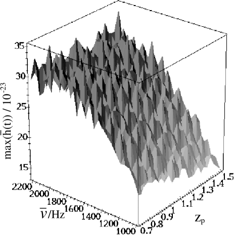
Figure 3: Three-surface showing the peak measured signal at the detector outputs (after data processing), ${\rm max}(\bar{h}(t))$, as a function of the peak redshift, $z_{\rm p}$, and the mean source frame frequency, $\bar{\nu}$, for the NS–NS model with MPD redshift distribution. Model parameters are described in Section 3. We used a mean total emitted GW energy at the source of $F=10^{52}{\rm~{}ergs}$ but the vertical axis can be scaled as $\sqrt{F}$ for generalization to other values.

In Fig. 4 we show results for a similar set of parameters (see Section 3) but we use the PLFS redshift distribution. We note the immediate qualitative difference in that the results show less variation in $z_{p}$ space and that there is a linear increase in the signal with increasing frequency. This is similar to the almost linear increase we see in Fig. 3 (for the MPD model) at low frequencies and is due to the fact that more sources lie at higher redshift in the PLFS model. That is, the frequency of the leveling off will be higher since the GWs, on the average, at an average redshift in the PLFS model, are redshifted below the resonance band in the detector. Quantitatively though, the PLFS model provides a lower average flux in the resonance band, and we see that the signal is $\sim 1/2$ that given by the MPD model throughout the parameter space.

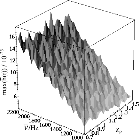
Figure 4: Three-surface showing the peak measured signal at the detector outputs, ${\rm max}(\bar{h}(t))$, as a function of the peak redshift, $z_{p}$, and the mean source frame frequency, $\bar{\nu}$, for the NS–NS model with PLFS redshift distribution. Model parameters are described in Section 3. We used a mean total emitted GW energy at the source of $F=10^{52}{\rm~{}ergs}$ but the vertical axis can be scaled as $\sqrt{F}$ for generalization to other values.

Finally, in Figs. 5 and 6, we provide the results for the quasar model. For Fig. 5 we used a uniform frequency distribution at the source with an order of magnitude width. All other parameters are kept the same as those used for the NS–NS models with the exception of the range of redshift parameter used. Fig. 6 shows a similar calculation using a Gaussian frequency distribution with the same width ($\sigma=500{\rm~{}Hz}$) as those used in the NS–NS models. We see a much slower variation of the signal over the parameter space, particularly at lower frequencies. Quantitatively, we see that the quasar models have comparative signal level with the star formation models and so we find that the signal seen at the bar detector is reasonably insensitive to the redshift and source model.

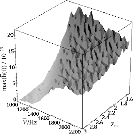
Figure 5: Three-surface showing the peak measured signal at the detector outputs, ${\rm max}(\bar{h}(t))$, as a function of the mean redshift, $z_{\rm m}$, and the mean source frame frequency, $\bar{\nu}$, for the quasar model. Model parameters are described in the text and are set so that we may compare these results with those in Figs. 3 and 4. In particular, we used a mean total emitted GW energy at the source of $F=10^{52}{\rm~{}ergs}$ but the vertical axis can be scaled as $\sqrt{F}$ for generalization to other values. However, here we have assumed a uniform frequency profile at the source with a width of an order of magnitude.

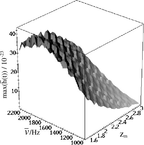
Figure 6: Three-surface showing the peak measured signal at the detector outputs, ${\rm max}(\bar{h}(t))$, as a function of the mean redshift, $z_{\rm m}$, and the mean source frame frequency, $\bar{\nu}$, for the quasar model. Model parameters are described in the text and are set so that we may compare these results with those in Figs. 3 and 4. Note that, in this case, we also keep the frequency profile as a Gaussian with $\sigma=500{\rm~{}Hz}$ at the source. Also, we used a mean total emitted GW energy at the source of $F=10^{52}{\rm~{}ergs}$ but the vertical axis can be scaled as $\sqrt{F}$ for generalization to other values.

We may compare the results in Figs. $2$–$6$ with the sensitivity curves provided by Tobar et al. (1995) for the NIOBE bar detector. The sensitivity curves show that, within the two resonance bands, the root-mean-square noise reaches a level of $\sim 2$ and $\sim 7\times 10^{-20}$, for the plus and minus mode respectively. For 1000 co-added bursts, the noise rises by a factor of $\sqrt{1000}$; $\sim 6$ and $\sim 22\times 10^{-19}$ in each band respectively. However, the maximum signals calculated in Figs. $3$–$6$ only range from $16$–$31\times 10^{-23}$. That is, the maximum expected signal-to-noise ratio after co-addition is $\sim 3\times 10^{-4}$. Therefore, despite the potential gain in signal evident in the co-addition results above, the NIOBE detector and other bar detectors, will still be unable to detect the signal with 1000 GRB times and existing GW data.

However, plans exist for improvements to be made to the NIOBE detector. A 2-mode sapphire transducer is to replace the existing vibration sensors and the cryogenic amplifier is to be significantly improved. In addition, the (microwave source) pump oscillator driving the transducer is to be improved. Tobar et al. (1998) report that these changes will decrease the detector noise to $\sim 5\times 10^{-21}$ in strain. A more important parameter will be the increase in the bandwidth of the detector from $\sim 0.3{\rm~{}Hz}$ in two bands to a single band with a width of $\sim 50{\rm~{}Hz}$. We discuss the prospects for the improved detector in Section 5.

5 Conclusions

Using models of the GW/GRB source and the spacetime distribution of sources, we have estimated the signal seen in the processed data of a typical bar detector, NIOBE. Assuming a knowledge of the time of the GW bursts (in this case, by assuming an association between GW and GRBs) allows us to co-add simulated GW data from many bursts. Figs. $3$–$6$ show the variation of the resultant signal with the main source parameter, the mean GW frequency $\bar{\nu}$, and the main spacetime parameter, the peak or mean redshift, $z_{p}$ or $z_{\rm m}$. These results assume co-addition of 1000 measured burst events. The largest signal that can be expected occurs within the NS–NS model with the MPD redshift distribution. The peak in signal occurs over a large region of parameter space covering mean rest frame GW frequencies $\bar{\nu}\mathrel{\hbox to0.0pt{\lower 3.0pt\hbox{$\mathchar 536\relax$}\hss}\raise 2.0pt\hbox{$\mathchar 318\relax$}}1600{\rm~{}Hz}$ and all realistic peak redshifts $z_{p}$. The maximum expected SNR is $\sim 5\times 10^{-4}$ in this case. Thus, comparing the signal with the noise floor of NIOBE, we find that the co-addition, with the present sensitivity of NIOBE and the present number of bursts, is insufficient to allow detection by a method based on the formalism in Section 2.

However, the improvements to NIOBE will result in an order of magnitude sensitivity gain. The bandwidth will also increase by a factor $50.0/(2\times 0.3)=83$. Tobar & Blair (1995) and Tobar (1997) report that, to a good approximation, $h\propto\sqrt{\Delta f}$ for $\Delta f$ the bandwidth of the detector. That is, from Eq. 8, a linear change in the cross section of the bar, $\Sigma_{\nu_{0}^{\prime}}$, corresponds to a change in $h\propto\sqrt{\Sigma_{\nu_{0}^{\prime}}}$. We can therefore find an optimistic estimate of the number of bursts, $N_{\rm b}$, required for us to achieve a SNR $\sim 1$,

$$\begin{array}[]{ll}N_{\rm b}\sim&1000\left(\frac{1}{5\times 10^{-4}}\right)^{2}\left(\frac{S_{\rm new}}{3\times 10^{-20}}\right)^{2}\left(\frac{1}{\Gamma(10{\rm s})}\right)^{2}\\ &\left(\frac{10^{52}{\rm~{}ergs}}{F}\right)\left(\frac{0.6{\rm~{}Hz}}{\Delta f}\right)\,.\\ \end{array}$$ (11)

The first term reflects the fact that we have achieved a SNR $\sim 5\times 10^{-4}$ using 1000 co-added bursts. The second term takes account of an increase in sensitivity; $S_{\rm new}$ is the strain sensitivity in the resonance band of the improved detector. The final terms incorporate changes in the time lag factor introduced in Fig. 2, an increased average energy output in GWs at the source and a change in the bandwidth of the detector respectively. Thus, the number of GW/GRBs to be observed could be as low as $\sim 8000$–$10000$ in the best case. Under this assumption, detection of GWs by NIOBE could be found in $\sim 25$ years as the GRB detection rate is $\sim 1$ per day. A disadvantage here is that the accumulation of new observed bursts would start after the improvements are made to NIOBE and the already available data would be of very limited use.

An additional possibility is that similar improvements be made to other existing bar detectors. The data corresponding to GRB times from the five detectors could then be co-added and the time for a possible detection could reduce to only $25/\sqrt{5}\sim 10$ years assuming that all detectors cover all GW/GRB events and that they all achieve similar characteristics to the improved NIOBE detector.

Finn, Mohanty & Romano (1999) have independently suggested a similar idea to that presented in this article, regarding the future capabilities of the LIGO detectors. They suggest that correlating the output from two LIGO detectors previous to GRB times could result in a 95% confidence detection of an association between GRBs and GWs after the observation of $\sim 1000$ GRBs. If no signal is present then increased numbers of observed bursts could place limits on the possible mechanisms for GRBs. Conceivably, a detection could be possible within $4$–$5$ years of the beginning of full LIGO operation. However, if the GW waveform is known (i.e. the GW/GRB mechanism is determined to some degree), a detection of GWs may occur in less time since matched filtering could be used to analyse the signal more effectively.

The importance of the above results is clear. If improvements are made to existing bar detectors, a detection of GW/GRB association may be possible in a similar amount of time as for twin LIGO-like detectors using the technique outlined in Sections 2 and 3. Such detection, whether by bar detectors or by laser interferometers, may be the only observational technique available to place constraints on GRB mechanisms aside from measurements of fading optical GRB counterparts. This distinct advantage comes with the loss of polarisation information and information about the time delay between GW and gamma ray emission. These are, unfortunately, important parameters for distinguishing gamma ray burster models (Kochanek & Piran 1993). Also, despite the fact that the results in Figs. $3$–$6$ are quite distinct, our ability to distinguish the different model parameters is lost in the co-addition procedure. However, the importance of these losses is not great when we remind ourselves that GWs have still not been directly detected; both the lower cost improvements to existing bar detectors and the high cost development of LIGO detectors are of great importance to the study of GRBs.

References

-
[1]
Allen B., 1997, GRASP: a data analysis package for gravitational wave detection (LIGO Collaboration),
http://www.lsc-group.uwm.edu/ - [2] Allen B. et al., 1999, Phys. Rev. Lett., 83, 1498
- [3] Astone P. et al., 1993, Phys. Rev. D, 47, 362
- [4] Blanchet L., 1996, Phys. Rev. D, 54, 1417
- [5] Centrella J. M., McMillan S. L. W., 1993, ApJ, 416, 719
- [6] Cerdonio M et al., 1995, in Coccia E., Pizzella G., Ronga F., eds, Proc. First Edoardo Amaldi Conference on Gravitational Wave Experiments, World Scientific, Singapore, p. 176
- [7] Coccia E. et al., 1995, in Coccia E., Pizzella G., Ronga F., eds, Proc. First Edoardo Amaldi Conference on Gravitational Wave Experiments, World Scientific, Singapore, p. 161
- [8] Cutler C., Flanagan É. É., 1994, Phys. Rev. D, 46, 2658
- [9] Damour T., Iyer B. R., Sathyaprakash B. S., 1998, Phys. Rev. D, 57, 885
- [10] Dhurandhar S. V., Blair D. G., Costa M. E., 1996, A&A, 311, 1043
- [11] Djorgovski S. et al., 1998, GCN GRB Observation Report, 137
- [12] Dokuchaev V. I., Eroshenko Yu. N., Ozernoy L. M., 1998, ApJ, 502, 192
- [13] Finn L. S., Chernoff D. F., 1993, Phys. Rev. D, 47, 2198
- [14] Finn L. S., Mohanty S. D., Romano J. D., 1999, Phys. Rev. D, 60, 121101
- [15] Fishman G. J., Meegan C. A., 1995, ARA&A, 33, 415
- [16] Flanagan É, É, Hughes S. A., 1998, Phys. Rev. D, 57, 4535
- [17] Fryer C. L., Woosley S. E., Herant M., Davies M. B., 1999, ApJ, 520, 650
- [18] Heng I. S., Blair D. G., Ivanov E. N., Tobar M. E., 1996, Phys. Lett. A, 218, 190
- [19] Horak J. M., Emslie A. G., Hartmann D. H., 1995, ApJ, 447, 474
- [20] Hulse R. A., Taylor J. H., 1975, ApJ, 195, L51
- [21] Kidder L. E., Will C. M., Wiseman A. G., 1992, Class. Quantum Grav., 9, L125
- [22] Kidder L. E., Will C. M., Wiseman A. G., 1993, Phys. Rev. D, 47, 3281
- [23] Kochanek C. S., Piran T., 1993, ApJ, 417, L17
- [24] Krumholz M., Thorsett S. E., Harrison F. A., 1998, ApJ, 506, L81
- [25] Kulkarni S. et al., 1998, Nature, 393, 35
- [26] Lee W. H., Kluźniak W., 1998, in Coccia E., Pizzella G., Veneziano G., eds, Proc. Second Edoardo Amaldi Conference on Gravitational Waves, World Scientific, Singapore
- [27] Madau P., Pozzetti, L. and Dickinson, M., 1998, ApJ, 498, 106 (MPD)
- [28] Mauceli E. et al., 1996, Phys. Rev. D, 54, 1264
- [29] Metzger M. et al., 1997, Nature, 387, 879
- [30] Misner C. W., Thorne K. S., Wheeler J. A., 1973, Gravitation, Freeman, San Fransisco
- [31] Oohara K., Nakamura T., 1996, in Marck J. -A., Lasota J. -P., eds, Proc. Les Houches School, Astrophysical Sources of Gravitational Radiation, Cambridge University Press, England
- [32] Paciesas W. S. et al., 1999, ApJS, 122, 465
- [33] Paik H. J., Wagoner R. V., 1976, Phys. Rev. D, 13, 2694
- [34] Pascarelle S. M., Lanzetta K. M., Fernández-Soto, A., 1998, ApJ, 508, L1 (PLFS)
- [35] Piran T. et al., 1991, in Paciesas W. S., Fishman G. J., eds, Proc. Huntsville GRB Workshop, New York: AIP, 149
- [36] Rasio F. A., Shapiro S. L., 1992, ApJ, 401, 226
- [37] Ruffert M., Janka H. -Th., 1998, A&A, 338, 535
- [38] Thorne K. S., 1992, in Hawking S. W., Israel W., eds, Three hundred years of gravitation, Cambridge University Press, Great Britain
- [39] Thorne K. S., 1994, in Sasaki M., ed., Proc. of the 8th Nishinomiya-Yukawa Symposium on Relativistic Cosmology, Universal Acad. Press, Japan
- [40] Thorsett S. E., Chakrabarty D., 1999, ApJ, 512, 288
- [41] Tobar M. E. et al., 1995, Aust. J. Phys., 48, 1007
- [42] Tobar M. E., Blair D. G., 1995, Rev. Sci. Instrum., 66, 108
- [43] Tobar M. E., 1997, in Kuroda K., ed., Proc. of the international workshop on gravitation and astrophysics, University of Tokyo, Japan, p. 199
- [44] Tobar M. E., Ivanov E. N., Locke C. R., Blair D. G., 1998, in Coccia E., Pizzella G., Veneziano G., eds, Proc. Second Edoardo Amaldi Conference on Gravitational Waves, World Scientific, Singapore, p. 408
- [45] Totani T., 1997, ApJ, 486, L71
- [46] van Paradijs J., 1997, Nature, 386, 686
- [47] Weber J., 1960, Phys. Rev., 117, 306