Relaxation of Wobbling Asteroids and Comets. Theoretical Problems. Perspectives of Experimental Observation.

Abstract

A body dissipates energy when it freely rotates about any axis different from principal. This entails relaxation, i.e., decrease of the rotational energy, with the angular momentum preserved. The spin about the major-inertia axis corresponds to the minimal kinetic energy, for a fixed angular momentum. Thence one may expect comets and asteroids (as well as spacecraft or cosmic-dust granules) stay in this, so-called principal, state of rotation, unless they are forced out of this state by a collision, or a tidal interaction, or cometary jetting, or by whatever other reason. As is well known, comet P/Halley, asteroid 4179 Toutatis, and some other small bodies exhibit very complex rotational motions attributed to these objects being in non-principal states of spin. Most probably, the asteroid and cometary wobble is quite a generic phenomenon. The theory of wobble with internal dissipation has not been fully developed as yet. In this article we demonstrate that in some spin states the effectiveness of the inelastic-dissipation process is several orders of magnitude higher than believed previously, and can be measured, by the presently available observational instruments, within approximately a year span. We also show that in some other spin states both the precession and precession-relaxation processes slow down considerably. (We call it near-separatrix lingering effect.) Such spin states may evolve so slowly that they can mimic the principal-rotation state.

I Introduction

It was a surprise for mission experts when, in 1958, the Explorer satellite changed its rotation axis. The satellite, a very prolate body with four deformable antennas on it, was planned to spin about its least-inertia axis, but for some reason refused to do so. Later the reason was understood: on general grounds, the body should end up in the spin state that minimises the kinetic rotational energy, for a fixed angular momentum. The rotation state about the maximal-inertia axis is the one minimising the energy, whereas spin about the least-inertia axis corresponds to the maximal energy. As a result, the body must get rid of the excessive energy and change the spin axis. This explains the vicissitudes of the Explorer mission.

Similarly to spacecraft, a comet or an asteroid in a non-principal rotation mode will dissipate energy and will, accordingly, return to the stable spin (Black et al. 1999, Efroimsky & Lazarian 1999). Nevertheless, several objects were found in excited states of rotation. These are, for example, comet P/Halley (Sagdeev et al. 1989; Peale & Lissauer 1989; Peale 1991), comet 46P/Wirtanen (Samarasinha, Mueller & Belton 1996; Rickman & Jorda 1998), comet 29P/Schwachmann-Wachmann 1 (Meech et al 1993), asteroid 1620 Geographos (Prokof’eva et al. 1997; Prokof’eva et al. 1996), and asteroid 4179 Toutatis (Ostro et al. 1993, Harris 1994, Ostro et al. 1995, Hudson and Ostro 1995, Scheeres et al. 1998, Ostro et al. 1999).

The dynamics of a freely rotating body is determined, on the one hand, by the initial conditions of the object’s formation and by the external factors forcing the body out of its principal spin state. On the other hand, it is influenced by the internal dissipation of the excessive kinetic energy associated with wobble. Two mechanisms of internal dissipation are known. The so-called Barnett dissipation, caused by the periodic remagnetisation, is relevant only in the case of cosmic-dust-granule alignment (Lazarian & Draine 1997). The other mechanism, called inelastic relaxation, is also relevant for mesoscopic grains, and plays a primary role in the case of macroscopic bodies

Inelastic relaxation results from the alternating stresses that are generated inside a wobbling body by the transversal and centripetal acceleration of its parts. The stresses deform the body, and inelastic effects cause energy dissipation.

The external factors capable of driving a rotator into an excited state are impacts and tidal interactions, the latter being of a special relevance for planet-crossers. In the case of comets, wobble is largely caused by jetting. Even gradual outgassing may contribute to the effect because a spinning body will start tumbling if it changes its principal axes through a partial loss of its mass or through some redistribution thereof. Sometimes the entire asteroid or comet may be a wobbling fragment of a progenitor disrupted by a collision (Asphaug & Scheeres 1999, Giblin & Farinella 1997, Giblin et al. 1998) or by tidal forces. All these factors that excite rotators compete with the inelastic dissipation that always tends to return the rotator back to the fold.

Study of rotation of small bodies may provide much information about their recent history and internal structure. However, theoretical interpretation of the observational data will become possible only after we understand quantitatively how inelastic dissipation affects rotation.

Evidently, the kinetic energy of rotation will decrease at a rate equal to that of energy losses in the material. Thus one should first calculate the elastic energy stored in a tumbling body, and then calculate the energy-dissipation rate, using the material quality factor $\,Q$. This empirical factor is introduced for a phenomenological description of the overall effect of the various attenuation mechanisms (Nowick & Berry 1972; Burns 1986, 1977; Knopoff 1963; Goldreich & Soter 1965). A comprehensive discussion of the $Q$-factor of asteroids and of its frequency- and temperature-dependence is presented in Efroimsky & Lazarian (2000).

A pioneer attempt to study inelastic relaxation in a wobbling asteroid was made by Prendergast back in 1958. Prendergast (1958) pointed out that the precession-caused acceleration must create fields of stress and strain over the body volume. He did not notice the generation of the higher-than-the-second harmonics, but he did point out the presence of the second harmonic: he noticed that precession with rate $\;\omega\;$ produces stresses of frequency $\;2\,\omega\;$ along with those of $\;\omega\;$. Since Prendergast’s calculation was wrong in several respects (for example, he missed the term $\;{\dot{\bf\Omega}}\,\times\,{\bf r}\;$), it gave him no chance to correctly evaluate the role of nonlinearity, i.e., to estimate the relative contribution of the harmonics to the entire effect, a contribution that is sometimes of the leading order. Nonetheless, Prendergast should be credited for being the first to notice the essentially nonlinear character of the inelastic relaxation. Another publication where the emergence of the second harmonic was pointed out was by Peale (1973) who addressed inelastic relaxation in the case of nearly spherical bodies. This key observation made by Prendergast and Peale went unnoticed by colleagues and was forgotten, even though their papers were once in a while mentioned in the references. Later studies undertaken by Burns & Safronov (1973), for asteroids, and by Purcell (1979), for cosmic-dust granules, treated the issue from scratch and fully ignored not only the higher harmonics but even the second mode $\;2\,\omega\;$. This led them to a several-order-of-magnitude underestimation of the effectiveness of the process, because the leading effect comes often from the second mode and sometimes from higher modes. One more subtlety, missed by everyone who ever approached this problem, was that, amazingly, the harmonics $\;\omega_{n}\,=\,n\,\omega_{1}\;$ are not necessarily multiples of the precession rate $\,\bf{\omega}\,$. We shall demonstrate that in fact a body precessing at rate $\,\omega\,$ experiences a superposition of stresses alternating at frequencies $\;\omega_{n}\,=\,n\,\omega_{1}\,$. Here the ”base frequency”  $\,\omega_{1}\,$ can either coincide with the precession rate $\,\omega\,$ or be lower than it, dependent upon the symmetry of the top and upon its rotation state. (For example, $\,\omega_{1}\,$ coincides with $\,\omega\,$ in the case of symmetrical oblate rotator. In this special case, $\,\omega_{1}\,$ itself and $\,\omega_{2}\,=\,2\,\omega_{1}\,=\,2\,\omega\,$ are the only emerging harmonics. But in the general case of a triaxial top all the other harmonics will show themselves.)

Another oversight present in all the afore-quoted studies was their mishandling of the boundary conditions. In Purcell’s article, where the body was modelled by an oblate rectangular prism, the normal stresses had their maximal values on the free surfaces and vanished in the centre of the body (instead of being maximal in the centre and vanishing on the surfaces). In Burns & Safronov (1973) the boundary conditions, at first glance, were not touched upon at all. In fact, they were addressed tacitly when the authors tried to decompose the pattern of deformations into bending and bulge flexing. An assumption adopted in Burns & Safronov (1973), that “the centrifugal bulge and its associated strains wobble back and forth relative to the body as the rotation axis $\;\bf\omega\;$ moves through the body during a wobble period,” lead the authors to a misconclusion that the “motion of the bulge through the (nutation) angle $\;\alpha\;$ produces strain energy” and to a calculation based thereon. In reality, however, the bulge appearance is but an iceberg tip, in that an overwhelming part of the inelastic dissipation process is taking place not near the surface but in the depth of the body, deep beneath the bulge. This follows from the fact that the stress and strain are small in the shallow regions and increase in the depth, if the boundary conditions are improved. (Remarkably, in the Peale, Cassen and Reynolds (1979) discussion of tidal dissipation in Io, maximum dissipation was also found to occur in the centre of the initially solid Io.)

II Notations and Assumptions

We shall use two coordinate systems. The body frame will naturally be represented by the three principal axes of inertia: $1$, $2$, and $3$, with coordinates $x$, $y$, $z$, and unit vectors ${\bf{e}}_{1}$, ${\bf{e}}_{2}$, ${\bf{e}}_{3}$. The second (inertial) frame ($X$, $Y$, $Z$), with basis vectors ${\bf{e}}_{X}$, ${\bf{e}}_{Y}$, ${\bf{e}}_{Z}$, may be chosen with its $Z$ axis aimed along the body’s angular-momentum vector $\bf{J}$ and with its origin coinciding with that of the body frame (i.e., with the centre of mass). The inertial-frame coordinates will be denoted by the same capital letters: $X$, $Y$, and $Z$ as the axes.

The angular momentum $\bf{J}$ of a freely-precessing body is conserved in the inertial frame. The body-frame-related components of the inertial angular velocity $\bf{\Omega}$ will be called $\;\Omega_{1,2,3}\;$, while letter $\;\omega\;$ will be reserved for the precession rate.

A body-frame-based observer will view both the inertial angular velocity $\;{\bf{\Omega}}\;$ and the angular momentum $\;\bf J\;$ nutating around the principal axis $\;3\;$ at rate $\;\omega\,$. An inertial observer, though, will argue that it is rather axis $3$ and angular velocity $\;\bf\Omega\;$ that are wobbling about $\bf{J}$. As is well known, the precession rate of $\;\bf\Omega\;$ about $\;\bf J\;$ in the inertial frame is different from the precession rate $\;\omega\;$ of $\;\bf\Omega\;$ about axis $\;3\;$ in the body frame. (See Section IV.) We would emphasize that the precession rate of our interest is the one in the body frame.

Free rotation of a body is described by Euler’s equations

$$\frac{d}{dt}\;\left(I_{i}\;\Omega_{i}\right)\;=\;\left(I_{j}\;-\;I_{k}\right)\;\Omega_{j}\;\Omega_{k}\;\;\;,\;\;\;$$ (1)

$(ijk)\,$ being a cyclic transposition of $\,(123)$, and the principal moments of inertia ranging as

$$I_{1}\;\leq\;I_{2}\;\leq\;I_{3}\;\;\;\;.$$ (2)

Since no uniform concensus on notations exists in the literature, the following table may simplify reading:

	Principal moments	Components of the angular	Rate of angular-velocity wobble,
	of inertia	velocity in the body frame	in the body frame
(Purcell 1979),
(Lazarian &
Efroimsky 1999),
(Efroimsky 2000),
(Efroimsky &	$I_{3}\;\geq\;I_{2}\;\geq\;I_{1}$	$\Omega_{3}\;\;,\;\;\;\Omega_{2}\;\;,\;\;\;\Omega_{1}$	$\omega$
Lazarian 2000),
present article
(Synge & Griffiths 1959)	$A\geq B\geq C$	$\omega_{1}\;\;,\;\;\;\omega_{2}\;\;,\;\;\;\omega_{3}$	$p$
(Black et al. 1999)	$C\geq B\geq A$	$\omega_{c}\;\;,\;\;\;\omega_{b}\;\;,\;\;\;\omega_{a}$	$\nu$

In the body frame, the period of angular-velocity precession about the principal axis $\;3\;$ is: $\;\tau\;=\;2\,\pi/\omega\,.$ Evidently,

$${\dot{\Omega}}_{i}/{\Omega}_{i}\;\approx\;{\tau}^{-1}\;\;\;,\;\;\;\;\;{\dot{I}}_{i}/{I}_{i}\;\approx\;{\tau}^{-1}\,\epsilon\;\;\;,\;\;\;$$ (3)

$\epsilon\;$ being a typical value of the relative strain that is several orders less than unity. These estimates lead to the inequality $\;\dot{I_{i}}\,\Omega_{i}\;\ll\;I_{i}\,\dot{\Omega_{i}}\;$, thereby justifying the commonly used approximation to Euler’s equations:

$$I_{i}\;{\dot{\Omega}}_{i}\;=\;\left(I_{j}\;-\;I_{k}\right)\;\Omega_{j}\;\Omega_{k}\;\;\;\;.$$ (4)

Thus it turns out that in our treatment the same phenomenon is neglected in one context and accounted for in another: on the one hand, the very process of the inelastic dissipation stems from the precession-inflicted small deformations; on the other hand, we neglect these deformations in order to write down (4). This approximation (also discussed in Lambeck 1988) may be called adiabatic, and it remains acceptable insofar as the relaxation is slow against rotation and precession. To cast the adiabatic approximation into its exact form, one should first come up with a measure of the relaxation rate. Clearly, this should be the time derivative of the angle $\;\theta\;$ made by the major-inertia axis $\;3\;$ and the angular momentum $\;\bf J\;$. The axis aligns towards $\;\bf J\;$, so $\;\theta\;$ must eventually decrease. Be mindful, though, that even in the absence of dissipation, $\;\theta\;$ does evolve in time, as can be shown from the equations of motion. Fortunately, this evolution is periodic, so one may deal with a time derivative of the angle averaged over the precession period. In practice, it turns out to be more convenient to deal with the squared sine of $\theta$ (Efroimsky 2000) and to write the adiabaticity assertion as:

$$-\;\frac{d\,\left\langle\sin^{2}\theta\right\rangle}{dt}\,\ll\,\omega\;\;,$$ (5)

$\omega$ being the precession rate and $\,<...>\,$ being the average over the precession period. The case of an oblate symmetrical top is exceptional, in that $\,\theta\,$ remains, when dissipation is neglected, constant over a precession cycle. No averaging is needed, and the adiabaticity condition simplifies to:

$$-\;\left(\frac{d\,\theta}{dt}\right)_{(oblate)}\,\ll\,\omega\;\;.$$ (6)

We would emphasise once again that the distinction between the oblate and triaxial cases, distinction resulting in the different forms of the adiabaticity condition, stems from the difference in the evolution of $\,\theta\,$ in the weak-dissipation limit. The equations of motion of an oblate rotator show that, in the said limit, $\,\theta\,$ stays virtually unchanged through a precession cycle (see section IV below). So the slow decrease of $\,\theta\,$, accumulated over many periods, becomes an adequate measure for the relaxation rate. The rate remains slow, compared to the rotation and precession, insofar as (6) holds. In the general case of a triaxial top the equations of motion show that, even in the absence of dissipation, angle $\,\theta\,$ periodically evolves, though its average over a cycle stays unchanged (virtually unchanged, when dissipation is present but weak). In this case we should measure the relaxation rate by the accumulated, over many cycles, change in the average of $\,\theta\,$ (or of $\,\sin^{2}\theta\,$). Then our assumption about the relaxation being slow yields (5)

The above conditions (5) - (6) foreshadow the applicability domain of our further analysis. For example, of the two quantities,

$$I_{1}^{2}\,{\Omega}_{1}^{2}\;+\;I_{2}^{2}\,{\Omega}_{2}^{2}\;+\;I_{3}^{2}\,{\Omega}_{3}^{2}\;=\;{\bf{J}}^{2}\;\;\;,\;\;$$ (7)

$$I_{1}\,{\Omega}_{1}^{2}\;+\;I_{2}\,{\Omega}_{2}^{2}\;+\;I_{3}\,{\Omega}_{3}^{2}\;=\;2\;T_{{kin}}\;\;\;,\;\;$$ (8)

only the former will conserve exactly, while the latter will remain virtually unchanged through one cycle and will be gradually changing through many cycles (just like $\;\;\left\langle\sin^{2}\theta\right\rangle\;\,$).

III The strategy

As mentioned above, in the case of an oblate body, when the moments of inertia relate as $\;I_{3}\;>\;I_{2}\;=\;I_{1}\;$, the angle $\;\theta\;$ between axis 3 and $\;\bf J\;$ remains adiabatically unchanged over the precession cycle. Hence in this case we shall be interested in $\dot{\theta}$, the rate of the maximum-inertia axis’ approach to the direction of $\bf{J}$. In the general case of a triaxial rotator, angle $\;\theta\;$ evolves through the cycle, but its evolution is almost periodic and, thus, its average over the cycle remains virtually constant. Practically, it will turn out to be more convenient to use the average of its squared sine. In this case, the alignment rate will be characterised by the time derivative of $\;\;<\sin^{2}\theta>\;$. Evidently,

$$\frac{d\;<\sin^{2}\theta>}{dt}\;=\;\frac{d\;<\sin^{2}\theta>}{dT_{kin}}\;\;\frac{dT_{kin}}{dt}\;\;\;,\;\;\;\;$$ (9)

while for an oblate case, when $\,\theta\,$ remains virtually unchanged over a cycle, one would simply write:

$$\left(\frac{d\,\theta}{dt}\right)_{(oblate)}\;=\;\left(\frac{d\,\theta}{dT_{kin}}\right)_{(oblate)}\;\;\frac{dT_{kin}}{dt}\;\;\;.\;\;\;\;$$ (10)

The derivative $\;d\,<\sin^{2}\theta>/dT_{kin}\,$ appearing in (9), as well as $\,\left(d\,\theta/dT_{kin}\right)_{(oblate)}\,$ appearing in (10), can be calculated from (7), (8) and the equations of motion. These derivatives indicate how the losses of the rotational energy affect the value of $\;<\sin^{2}\theta>\;$ (or simply of $\theta$, in the oblate case). The kinetic-energy decrease is caused by the inelastic dissipation,

$$\dot{T}_{kin}\;=\;<\dot{W}>\;\;\;,\;\;\;$$ (11)

$W\;$ being the elastic energy of the alternating stresses, and $\;<W>\;$ being its average over a precession cycle. This averaging is justified within our adiabatic approach. So we shall eventually deal with the following formulae for the alignment rate:

$$\frac{d\,<\sin^{2}\theta>}{dt}\;=\;\frac{d\,<\sin^{2}\theta>}{dT_{kin}}\;\;\frac{d\,<W>}{dt}\;\;\;,\;\;\;$$ (12)

in the general case, and

$$\left(\frac{d\,\theta}{dt}\right)_{(oblate)}\;=\;\left(\frac{d\,\theta}{dT_{kin}}\right)_{(oblate)}\;\;\frac{d\,<W>}{dt}\;\;\;,\;\;\;\;$$ (13)

for an oblate rotator.

Now we are prepared to set out the strategy of our further work. While calculation of $\;d{\left\langle\right.}\sin^{2}\theta{{\left.\right\rangle}}/dT_{kin}\;$ and $\;\left(d\theta/dT_{kin}\right)_{oblate}\;$ is an easy exercise, our main goal will be to find the dissipation rate $\;d\,<W>/dt\;$. This quantity will consist of inputs from the dissipation rates at all the frequencies involved in the process, i.e., from the harmonics at which stresses oscillate in a body precessing at a given rate $\,\omega\,$. The stress is a tensorial extension of the notion of a pressure or force. Stresses naturally emerge in a spinning body due to the centripetal and transversal accelerations of its parts. Due to the precession, these stresses contain time-dependent components. If we find a solution to the boundary-value problem for alternating stresses, it will enable us to write down explicitly the time-dependent part of the elastic energy stored in the wobbling body, and to separate contributions from different harmonics:

$$<W>\;=\;\sum_{n}\;\,<W(\omega_{n})>\;\;\;\;\;.\;\;$$ (14)

$W(\omega_{n})\;$ being the elastic energy of stresses alternating at frequency $\,\omega_{n}$. One should know each contribution $W(\omega_{n})$, for these will determine the dissipation rate at the appropriate frequency, through the frequency-dependent empirical quality factors. The knowledge of these factors, along with the averages $\,<W(\omega_{n})>\,$, will enable us to find the dissipation rates at each harmonic. Sum of those will give the entire dissipation rate due to the alternating stresses emerging in a precessing body.

IV Inelastic Dissipation

Equation $(\ref{4.9})$ implements the most important observation upon which all our study rests: generation of harmonics in the stresses inside a precessing rigid body. The harmonics emerge because the acceleration of a point inside a precessing body contains centrifugal terms that are quadratic in the angular velocity $\bf{\Omega}$. In the simpliest case of a symmetrical oblate body, for example, the body-frame-related components of the angular velocity are given in terms of $\,\sin\omega t\,$ and $\,\cos\omega t\,$ (see formulae (25) from Section V). Evidently, squaring of $\bf{\Omega}$ will yield terms both with $\,\sin\omega t\,$ or $\,\cos\omega t\,$ and with $\,\sin 2\omega t\,$ or $\,\cos 2\omega t\,$. The stresses produced by this acceleration will, too, contain terms with frequency $\,\omega t\,$ as well as those with the harmonic $\,2\omega t$. In the further sections we shall explain that a triaxial body precessing at rate $\,\omega\,$ is subject, in distinction from a symmetrical oblate body, to a superposition of stresses oscillating at frequencies $\;\omega_{n}\,=\,n\,\omega_{1}\,$, the ”base frequency” $\,\omega_{1}\,$ being lower than the precession rate $\,\omega$. The basic idea is that in the general, non-oblate case, the time dependence of the acceleration and stresses will be expressed not by trigonometric but by elliptic functions whose expansions over the trigonometric functions will generate an infinite number of harmonics.

The total dissipation rate will be a sum of the particular rates (Stacey 1992) to be calculated empirically. The empirical description of attenuation is based on the quality factor $\,Q(\omega)\,$ and on the assumption of attenuation rates at different harmonics being independent from one another:

$$\dot{W}\;=\;\sum_{n}\;\dot{W}{({\omega_{n}})}\;=\;-\;\sum_{n}\;\frac{\omega_{n}\;W_{0}({\omega}_{n})}{Q({\omega_{n}})}\;=\;-\;2\;\sum_{n}\;\frac{\omega_{n}\;\,<W({\omega}_{n})>}{Q({\omega_{n}})}\;\;\;\;\\$$ (15)

$\;Q(\omega)\;$ being the quality factor of the material, and $\;W_{0}({\omega}_{n})\;$ and $\;\,<W({\omega}_{n})>\,\;$ being the maximal and the average values of the appropriate-to-$\omega_{n}\;$ fraction of elastic energy stored in the body. This expression will become more general if we put the quality factor under the integral, implying its possible coordinate dependence:

$$\dot{W}\;=\;-\;2\;\sum_{\omega_{n}}\;\int\;dV\;\left\{\frac{\omega_{n}}{Q({\omega_{n}})}\;\,\frac{d\,<W(\omega_{n})>}{dV}\;\right\}\;\;\;,\;\;$$ (16)

The above assumption of attenuation rates at different harmonics being mutually independent is justified by the extreme smallness of strains (typically, much less than $\;10^{-6}$) and by the frequencies being extremely low ($10^{-5}\,-\,10^{-3}\;Hz$). One, thus, may say that the problem is highly nonlinear, in that we shall take into account the higher harmonics in the expression for stresses. At the same time, the problem remains linear in the sense that we shall neglect any nonlinearity stemming from the material properties (in other words, we shall assume that the strains are linear function of stresses). We would emphasize, though, that the nonlinearity is most essential, i.e., that the harmonics $\;\omega_{n}\;$ come to life unavoidably: no matter what the properties of the material are, the harmonics do emerge in the expressions for stresses. Moreover, as we shall see, the harmonics interfere with one another due to $\;W\;$ being quadratic in stresses. Generally, all the infinite amount of multiples of $\;\omega_{1}\;$ will emerge. The oblate case, where only $\;\omega_{1}\;$ and $\;2\omega_{1}\;$ show themselves, is an exception. Another exception is the narrow-cone precession of a triaxial rotator studied in Efroimsky (2000): in the narrow-cone case, only the first and second modes are relevant (and $\,\omega_{1}\,\approx\,\omega$).

Often the overall dissipation rate, and therefore the relaxation rate is determined mostly by harmonics rather than by the principal frequency. This fact was discovered only recently (Efroimsky & Lazarian 2000, Efroimsky 2000, Lazarian & Efroimsky 1999), and it led to a considerable re-evaluation of the effectiveness of the inelastic-dissipation mechanism. In some of the preceding publications, its effectiveness had been underestimated by several orders of magnitude, and the main reason for this underestimation was neglection of the second and higher harmonics. As for the choice of values of the quality factor $\;Q\,$, Prendergast (1958) and Burns & Safronov (1973) borrowed the terrestial seismological data for $Q$. In Efroimsky & Lazarian (2000), we argue that these data are inapplicable to asteroids.

To calculate the afore mentioned average energies $\,<W(\omega_{n})>\,$, we use such entities as stress and strain. As already mentioned above, the stress is a tensorial generalisation of the notion of pressure. The strain tensor is analogous to the stretching of a spring (rendered in dimensionless fashion by relating the displacement to the base length). Each tensor component of the stress consists of two inputs, elastic and plastic. The former is related to the strain through the elasticity constants of the material; the latter is related to the time-derivative of the strain, through the viscosity coefficients. As our analysis is aimed at extremely small deformations of cold bodies, the viscosity may well be neglected, and the stress tensor will be approximated, to a high accuracy, by its elastic part. Thence, according to Landau & Lifshitz (1976), the components of the elastic stress tensor $\sigma_{\it{ij}}$ are interconnected with those of the strain tensor $\epsilon_{\it{ij}}$ like:

$$\epsilon_{ij}\;\;=\;\;\delta_{ij}\;\;\frac{Tr\;\sigma}{9\;K}\;\;+\;\;\left(\;\sigma_{\it{ij}}\;\;-\;\;\frac{1}{3}\;\;\delta_{ij}\;\;Tr\;\sigma\right)\;\frac{1}{2\;\mu}\;\;\;~{}~{}~{},$$ (17)

$\mu$ and $K$ being the adiabatic shear and bulk moduli, and $Tr$ standing for the trace of a tensor.

To simplify the derivation of the stress tensor, the body will be modelled by a rectangular prism of dimensions $\,2\,a\,\times\,2\,b\,\times\,2\,c\,$ where $\,a\,\geq\,b\,\geq\,c$. The tensor is symmetrical and is defined by

$$\partial_{i}\sigma_{ij}\;=\;\rho\;a_{j}\;\;,\;\;$$ (18)

$a_{j}$ being the time-dependent parts of the acceleration components, and $\,\rho\,a_{j}$ being the time-dependent parts of the components of the force acting on a unit volume. Besides, the tensor $\,\sigma_{ij}$ must obey the boundary conditions: its product by normal unit vector, $\,\sigma_{ij}n_{j}\,$, must vanish on the boundaries of the body (this condition was not fulfilled in Purcell (1979)).

Solution to the boundary-value problem provides such a distribution of the stresses and strains over the body volume that an overwhelming share of dissipation is taking place not near the surface but in the depth of the body. For this reason, the prism model gives a good approximation to realistic bodies. Still, in further studies it will be good to generalise our solution to ellipsoidal shapes. Such a generalisation seems to be quite achievable, judging by the recent progress on the appropriate boundary-value problem (Denisov & Novikov 1987).

Equation (18) has a simple scalar analogue Consider a non-rotating homogeneous liquid planet of radius $\,R\,$ and density $\,\rho\,$. Let $\;g(r)\;$ and $\,P(r)\,$ be the free-fall acceleration and the self-gravitational pressure at the distance $\,r\,\leq\,R\,$ from the centre. (Evidently, $\,g(r)\,=\,(4/3)\,\pi\,G\,\rho\,r\,$.) Then the analogue to (18) will read:

$$\rho\;g(r)\;=\;-\;\frac{\partial P(r)}{\partial r}\;\;\;\;\;\;,\;\;\;\;$$ (19)

the expression $\;\rho\,g(r)\;$ standing for the gravity force acting upon a unit volume, and the boundary condition being $\;P(R)\,=\,0$. Solving equation (19) reveals that the pressure has a maximum at the centre of the planet, although the force is greatest at the surface. Evidently, the maximal deformations (strains) also will be experienced by the material near the centre of the planet.

In our case, the acceleration $\,\bf a\,$ of a point inside the precessing body will be given not by the free-fall acceleration $\,g({\bf{r}})\,$ but will be a sum of the centripetal and transversal accelerations: $\,{\bf{\Omega}}\,\times\,({\bf{\Omega}}\,\times\,{\bf{r}})\,+\,{\bf{\dot{\Omega}}}\,\times\,{\bf{r}}\;$, the Coriolis term being negligibly small. Thereby, the absolute value of $\,{\bf{a}}\,$ will be proportional to that of $\,\bf r\,$, much like in the above example. In distinction from the example, though, the acceleration of a point inside a wobbling top will have both a constant and a periodic component, the latter emerging due to the precession. For example, in the case of a symmetrical oblate rotator, the precessing components of the angular velocity $\,\bf\Omega\,$ will be proportional to $\,\sin\omega t\,$ and $\,\cos\omega t\,$, whence the transversal acceleration will contain frequency $\,\omega\,$ while the centripetal one will contain $\,2\omega$. The stresses obtained through (18) will oscillate at the same frequencies, and so will the strains. As we already mentioned, in the case of a non-symmetrical top an infinite amount of harmonics will emerge, though these will be obertones not of the precession rate $\,\omega\,$ but of some different ”base frequency” $\,\omega_{1}\,$ that is less than $\,\omega.$

Here follows the expression for the (averaged over a precession period) elastic energy stored in a unit volume of the body:

$$\frac{d\;\,<W>}{dV}\;=\;\frac{1}{2}\;\,<\epsilon_{ij}\;\sigma_{ij}>\;=\;\frac{1}{4\mu}\;\left\{\left(\frac{2\;\mu}{9\;K}\;-\;\frac{1}{3}\right)\;\,<\,\left(Tr\;\sigma\right)^{2}\,>\;+\;<\sigma_{ij}\,\sigma_{ij}>\right\}\;=$$ (20)

(21)

$$\frac{1}{4\mu}\;\left\{\,-\,\frac{1}{1\,+\,\nu^{-1}}\;\,<\left(Tr\;\sigma\right)^{2}>\,+\,<\sigma_{xx}^{2}>\,+\,<\sigma_{yy}^{2}>\,+\,<\sigma_{zz}^{2}>\,+\,2\,<\,\sigma_{xy}^{2}\,+\,\sigma_{yz}^{2}\,+\,\sigma_{zx}^{2}\,>\right\}\;\;$$ (22)

where $2\mu/(9K)-1/3=-\nu/(1+\nu)\approx-1/5$, $\,\nu$ being Poisson’s ratio (for most solids $\,\nu\approx 1/4$). Naturally, the total averaged elastic energy is given by the integral over the body’s volume:

$$<W>\;=\;\frac{1}{2}\;\int\;dV\;\sigma_{ij}\;\epsilon_{ij}\;\;\;\;,\;\;\;$$ (23)

and it must be expanded into the sum (14) of inputs from oscillations of stresses at different frequencies. Each term $\,\left\langle W(\omega_{n})\right\rangle\,$ emerging in that sum will then be plugged into the expression (15), together with the value of $\,Q\,$ appropriate to the overtone $\,\omega_{n}$.

V A Special Case: Precession of an Oblate Body.

An oblate body has moments of inertia that relate as:

$$I_{3}\;>\;I_{2}\;=\;I_{1}\;\equiv\;I\;\;.\;\;\;\;\;\;$$ (24)

We shall be interested in $\dot{\theta}$, the rate of the maximum-inertia axis’ approach to the direction of angular momentum $\bf{J}$. To achieve this goal, we shall have to know the rate of energy losses caused by the periodic deformation. To calculate this deformation, it will be necessary to find the acceleration experienced by a particle located inside the body at a point ($x$, $y$, $z$). Note that we address the inertial acceleration, i.e., the one with respect to the inertial frame $(X,Y,Z)$, but we express it in terms of coordinates $x$, $y$ and $z$ of the body frame $(1,2,3)$ because eventually we shall have to compute the elastic energy stored in the entire body (through integration of the elastic-energy density over the body volume).

The fast motions (revolution and precession) obey, in the adiabatical approximation, the simplified Euler equations (4). Their solution, with neglect of the slow relaxation, looks (Fowles and Cassiday 1986, Landau and Lifshitz 1976), in the oblate case (24):

$${\Omega}_{1}\;\;=\;\;{\Omega}_{\perp}\cos{\omega}t~{}~{},~{}~{}~{}{\Omega}_{2}\;\;=\;\;{\Omega}_{\perp}\sin{\omega}t~{}~{},~{}~{}~{}{\Omega}_{3}\;\;=\;\;const$$ (25)

where

$${{\Omega}_{\perp}}\;\;\equiv\;\;{\Omega}\;\;\sin\;{\alpha}~{}~{},~{}~{}~{}~{}~{}{{\Omega}_{3}}\;\;\equiv\;\;{\Omega}\;\;\cos\;{\alpha}\;\;\;,$$ (26)

$\;\alpha\;$ being the angle made by the major-inertia axis 3 with $\,\bf{\Omega}\,$. Expressions (25) show that in the body frame the angular velocity ${\bf{\Omega}}$ describes a circular cone about the principal axis $3$ at a constant rate

$$\omega\;=\;(h-1)\Omega_{3},\;\;\;\;\;\;\;\;h\equiv{I_{3}}/I~{}~{}~{}.$$ (27)

So angle $\;\alpha\;$ remains virtually unchanged through a cycle (though in the presence of dissipation it still may change gradually over many cycles). The precession rate $\;\omega\;$ is of the same order as $|{\bf{\Omega}}|$, except in the case of $\;h\,\rightarrow\,1\;$ or in a very special case of ${\bf{\Omega}}$ and ${\bf{J}}$ being orthogonal or almost orthogonal to the maximal-inertia axis $3$. Hence one may call not only the rotation but also the precession “fast motions” (implying that the relaxation process is a slow one). Now, let $\;\theta\;$ be the angle between the principal axis $3$ and the angular-momentum $\;\bf J\;$, so that $\;J_{3}\,=\,J\,\cos\theta\;$ and

$${\Omega}_{3}\;\;\equiv\;\;\frac{J_{3}}{I_{3}}\;\;=\;\;\frac{J}{I_{3}}\;\;\cos\;\theta~{}~{}~{}~{}~{}~{}$$ (28)

wherefrom

$$\omega\;=\;(h\;-\;1)\;\frac{J}{I_{3}}\;\cos\theta\;\;\;.$$ (29)

Since, for an oblate object,

$${\bf J}\,=\,I_{1}\,\Omega_{1}\,{\bf e}_{1}\,+\,I_{2}\,\Omega_{2}\,{\bf e}_{2}\,+\,I_{3}\,\Omega_{3}\,{\bf e}_{3}\,=\,I\,(\Omega_{1}\,{\bf e}_{1}\,+\,\Omega_{2}\,{\bf e}_{2})\,+\,I_{3}\,\Omega_{3}\,{\bf e}_{3}\,\;,\;$$ (30)

the quantity $\;\Omega_{\perp}\,\equiv\,\sqrt{\Omega_{1}^{2}+\Omega_{2}^{2}}\;$ is connected with the absolute value of $\bf J$ like:

$${\Omega}_{\perp}\;\;=\;\;\frac{J}{I}\;\;\sin\;\theta\;\;=\;\;\frac{J}{I_{3}}\;h\;\;\sin\;\theta\;\;\;,\;\;\;\;\;\;h\;\equiv\;I_{3}/I\;\;.\;\;$$ (31)

It ensues from (26) that $\;{{\Omega}_{\perp}}/{{\Omega}_{3}}\;=\;\tan\;\alpha\;$. On the other hand, (28) and (31) entail: $\;{{\Omega}_{\perp}}/{{\Omega}_{3}}\,=\,h\,\tan\,\theta\;$. Hence,

$$\tan\alpha\;=\;h\;\tan\theta\;\;\;.\;\;\;$$ (32)

We see that angle $\;\theta\;$ is almost constant too (though it gradually changes through many cycles). We also see from (30) that in the body frame the angular-momentum vector $\;\bf J\;$ describes a circular cone about axis $3$ with the same rate $\;\omega\;$ as $\;\Omega\;$. An inertial observer, though, will insist that it is rather axis $3$, as well as the angular velocity $\;\Omega\;$, that is describing circular cones around $\bf{J}$. It follows trivially from (27) and (30) that

$$I\;{\bf\Omega}\;=\;{\bf J}\;-\;I\;\omega\;{\bf e}_{3}\;\;\;,\;\;\;\;$$ (33)

whence it is obvious that, in the inertial frame, both $\bf\Omega$ and axis $\;3\;$ are precessing about $\bf J$ at rate $J/I$. (The angular velocity of this precession is ${\dot{\bf e}}_{3}\,=\,{\bf\Omega}\,\times\,{\bf e}_{3}\,=\,({\bf J}/I\,-\,\omega\,{\bf e}_{3})\,\times\,{\bf e}_{3}\,=\,({\bf J}/I)\,\times\,{\bf e}_{3}$.) Interestingly, the rate $\omega\,=\,(h\,-\,1)\,\Omega_{3}$, at which $\bf\Omega$ and $\bf J$ are precessing about axis $\;3\;$ in the body frame, differs considerably from the rate $J/I$ at which $\bf\Omega$ and axis $\;3\;$ are precessing around $\bf J$ in the inertial frame. (In the case of the Earth, $J/I\,\approx\,400\,\omega\;$ because $\,h\,$ is close to unity.) Remarkably, the inertial-frame-related precession rate is energy-independent and, thus, stays unchanged through the relaxation process. This is not the case for the body-frame-related rate $\,\omega\,$ which, according to (29), gradually changes because so does $\,\theta$.

As is explained above, we shall be interested in the body-frame-related components $\Omega_{1,2,3}$ precessing at rate $\omega$ about the principal axis $\;3$. Acceleration of an arbitrary point of the body can be expressed in terms of these components through formula

$${\bf{a}}\;\;=\;\;{\bf{a}}^{\prime}\;+\;{\bf{{\dot{\Omega}}}}\;\times\;{\bf{r}}^{\prime}\;+\;2\;{\bf{\Omega}}\;\times\;{\bf{v}}^{\prime}\;+\;{\bf{\Omega}}\;\times\;({\bf{\Omega}}\times{\bf{r}}^{\prime})\;\;\;\;,$$ (34)

where $\;{\bf{r}},\;{\bf{v}},\;{\bf{a}}\;$ are the position, velocity and acceleration in the inertial frame, and $\;{\bf{r}}^{\prime},\;{\bf{v}}^{\prime}\;$ and $\;{\bf{a}}^{\prime}\;$ are those in the body frame. Here $\;{\bf r}\,=\,{\bf r}^{\prime}\;$. Mind though that $\;{\bf{v}}^{\prime}\;$ and $\;{\bf{a}}^{\prime}\;$ do not vanish in the body frame. They may be neglected on the same grounds as term $\;{\dot{I}}_{i}\Omega_{i}\;$ in (1): precession of a body of dimensions $\;\sim\,{\it l}\;$, with period $\;\tau\;$, leads to deformation-inflicted velocities $\;v^{\prime}\,\approx\;\epsilon\,\it{l}/\tau\;$ and accelerations $\;a^{\prime}\,\approx\;\epsilon\,\it{l}/\tau^{2}\;$, $\;\epsilon\;$ being the typical order of strains arising in the material. Clearly, for very small $\;\epsilon\;$, quantities $\;v^{\prime}\;$ and $\;a^{\prime}\;$ are much less than the velocities and accelerations of the body as a whole (that are about $\;{\it{l}}/\tau\;$ and $\;{\it{l}}/{\tau}^{2}\;$, correspondingly). Neglecting these, we get, from (34) and (25), for the acceleration at point $\;(x,\,y,\,z)\;$:

$${\bf{a}}\;\;=\;\;{{\bf{e}}_{1}}\;\left\{\;{\frac{1}{2}}\;{\Omega}_{\perp}^{2}\;x\;\;\cos\;2{\omega}t\;\;+\;\;{\frac{1}{2}}\;{\Omega}_{\perp}^{2}\;y\;\;\sin\;2{\omega}t\;\;+\;\;z\;{\Omega}_{\perp}\;{\Omega}_{3}\;h\;\;\cos\;{\omega}t\;\right\}\;+$$ (35)

(36)

$$+\;\;{{\bf{e}}_{2}}\;\left\{{\frac{1}{2}}\;{\Omega}_{\perp}^{2}\;x\;\;\sin\;2{\omega}t\;\;-\;\;{\frac{1}{2}}\;{\Omega}_{\perp}^{2}\;y\;\;\cos\;2{\omega}t\;\;+\;\;z\;{\Omega}_{\perp}\;{\Omega}_{3}\;h\;\;\sin\;{\omega}t\;\;\right\}\;+$$ (37)

(38)

$$+\;\;{{\bf{e}}_{3}}\;\left\{{\Omega}_{\perp}\;{\Omega}_{3}\;(2\;-\;h)\;(x\;\;\cos\;{\omega}t\;\;+\;\;y\;\;\sin\;{\omega}t\;)\;\right\}~{}~{}~{}.$$ (39)

Plugging this into (18), with the proper boundary conditions imposed, yields, for an oblate prism of dimensions $\,2a\,\times\,2a\,\times\,2c\;$, $\;a\,>\,c\,$:

$$\sigma_{xx}=\frac{\rho\Omega_{\perp}^{2}}{4}(x^{2}-a^{2})\;\cos 2{\omega}t\;\;,\;\;\;\;\sigma_{yy}=-\frac{\rho\Omega_{\perp}^{2}}{4}(y^{2}-a^{2})\;\cos 2{\omega}t\;\;,\;\;\;\;\sigma_{zz}=0$$ (40)

$$\sigma_{xy}\;\;=\;\;\frac{\rho}{4}\;\Omega_{\perp}^{2}\;(x^{2}\;\;+\;\;y^{2}\;\;-\;\;2a^{2})\;\;\sin\;2{\omega}t\;\;\;,$$ (41)

$$\sigma_{xz}\;\;=\;\;\frac{\rho}{2}\;{\Omega_{\perp}}\;{\Omega_{3}}\;\left[\;h\;(z^{2}\;-\;c^{2})\;\;+\;\;(2\;-\;h)\;(x^{2}\;-\;a^{2})\;\right]\;\;\cos\;{\omega}t\;\;\;,$$ (42)

$$\sigma_{yz}\;\;=\;\;\frac{\rho}{2}\;{\Omega_{\perp}}\;{\Omega_{3}}\;\left[\;h\;(z^{2}\;-\;c^{2})\;\;+\;\;(2\;-\;h)\;(y^{2}\;-\;a^{2})\;\right]\;\;\sin\;{\omega}t\;\;\;.$$ (43)

In (39) - (43) we kept only time-dependent parts, because time-independent parts of the acceleration, stresses and strains are irrelevant in the context of dissipation. A detailed derivation of (39) - (43) is presented in (Lazarian & Efroimsky 1999).

Formulae (40) - (43) implement the polynomial approximation to the stress tensor. This approximation keeps the symmetry and obeys (18) with (39) plugged into it. The boundary condition are satisfied exactly for the diagonal components and only approximately for the off-diagonal components. The approximation considerably simplifies calculations and entails only minor errors in the numerical factors in (48).

The second overtone emerges, along with the principal frequency $\,\omega\,$, in the expressions for stresses since the centripetal part of the acceleration is quadratic in $\;\bf{\Omega}\;$. The kinetic energy of an oblate spinning body reads, according to (8), (26), and (32):

$$T_{kin}\;=\;\frac{1}{2}\;\left[I\;\Omega_{\perp}^{2}\;+\;I_{3}\;{\Omega_{3}}^{2}\right]\;=\;\frac{1}{2}\;\;\left[\;\frac{1}{I}\;\;\sin^{2}\;\theta\;\;+\;\;\frac{1}{I_{3}}\;\;\cos^{2}\;\theta\;\right]\;J^{2}\;\;,\;\;\;$$ (44)

wherefrom

$$\frac{dT_{kin}}{d\theta}\;\;=\;\;\frac{J^{2}}{I_{3}}\;(h\;-\;1)\;\;\sin\;\theta\;\;\cos\;\theta\;\;=\;\;\omega\;J\;\;\sin\;\theta\;\;\;.$$ (45)

The latter expression, together with (13) and (22), leads to:

$$\frac{d\theta}{dt}\;=\;\left(\frac{dT_{kin}}{d\theta}\right)^{-1}\frac{dT_{kin}}{dt}\;=\;\left(\omega\;J\;\;\sin\;\theta\right)^{-1}\;\dot{W}\;\;,$$ (46)

where

$$\dot{W}\;=\;\dot{W}^{({\omega})}\;+\;\dot{W}^{(2{\omega})}\;=\;\omega\;\frac{W_{0}^{({\omega})}}{Q^{({\omega})}}\;+\;2\;\omega\;\frac{W_{0}^{({2\omega})}}{Q^{({2\omega})}}\;\approx\;\frac{2\,\omega}{Q}\;\left\{<W^{({\omega})}>\;+\;2\;<W^{({2\omega})}>\right\}\;,$$ (47)

the quality factor assumed to depend upon the frequency very weakly. In the above formula, $\;W_{0}^{\omega}\;$ and $\;W_{0}^{2\omega}\;$ are amplitudes of elastic energies corresponding to the principal mode and the second harmonic. Quantities $<W^{\omega}>\,=\,W_{0}^{\omega}/2\,$ and $\,<W^{2\omega}>\,=\,W_{0}^{2\omega}/2\,$ are the appropriate averages. Substitution of (40) - (43) into (22), with further integration over the volume and plugging the result into (13), will give us the final expression for the alignment rate:

$$d\theta/dt\;=\;-\;\frac{3}{2^{4}}\;\sin^{3}\theta\;\;\frac{63\;(c/a)^{4}\;\cot^{2}\theta\;+\;20}{[1+(c/a)^{2}]^{4}}\;\;\frac{a^{2}\;\Omega^{3}_{0}\;\rho}{\mu\;Q}$$ (48)

where

$$\Omega_{0}\;\equiv\;\frac{J}{I_{3}}\;\;\;\;$$ (49)

is a typical angular velocity. Deriving (48), we took into account that, for an oblate $\;2a\,\times\,2a\,\times\,2c\;$ prism (where $\;a\,>\,c\;$), the moment of inertia $\;I_{3}\;$ and the parameter $\;h\;$ read:

$$I_{3}\;=\;\frac{16}{3}\;\rho\;a^{4}\;c\;\;\;\;\;,\;\;\;\;\;\;\;\;h\;\;\equiv\;\;\frac{I_{3}}{I}\;\;=\;\;\frac{2}{1\;+\;(c/a)^{2}}\;\;\;\;\;.\;\;\;$$ (50)

Details of derivation of (48) are presented in (Lazarian & Efroimsky 1999).

Formula (48) shows that the major-inertia axis slows down its alignment at small residual angles. For $\theta\rightarrow 0$, the derivative ${\dot{\theta}}\,$ becomes proportional to $\theta$, and thus, $\theta$ decreases exponentially slowly: $\theta=A\exp(-\zeta t)$, where $A$ and $\zeta$ are some positive numbers. This feature, ”exponentially slow finish”, (which was also mentioned, with regard to the Chandler wobble, in Peale (1973), formula (55)) is natural for a relaxation process, and does not lead to an infinite relaxation time if one takes into account the finite resolution of the equipment. Below we shall discuss this topic at length.

Another feature one might expect of (48) would be a “slow start”: it would be good if $\;d\theta/dt\;$ could vanish for $\;\theta\,\rightarrow\,\pi/2\;$. If this were so, it would mean that at $\;\theta\,=\,\pi/2\;$ (i.e., when the major-inertia axis is exactly perpendicular to the angular-momentum vector) the body “hesitates” whether to start aligning its maximal-inertia axis along or opposite to the angular momentum, and the preferred direction is eventually determined by some stochastic influence from the outside, like (say) a collision with a small meteorite. This behaviour is the simplest example of the famous spontaneous symmetry breaking, and in this setting it is desirable simply for symmetry reasons: $\;\theta\,=\,\pi/2\;$ must be a position of an unstable equilibrium. Contrary to these expectations, though, (48) leaves $\;d\theta/dt\;$ nonvanishing for $\;\theta\,\rightarrow\,\pi/2\;$, bringing an illusion that the major axis leaves the position $\;\theta=\pi/2\;$ at a finite rate. This failure of our formula (48) comes from the inapplicability of our analysis in the closemost vicinity of $\;\theta\,=\,\pi/2\;$. This vicinity simply falls out of the adiabaticity realm adumbrated by (6), because $\;\omega\;$ given by (29) vanishes for $\;\theta\,\rightarrow\,\pi/2\,$ (then one can no longer assume the relaxation to be much slower than the precession rate, and hence, the averaging over period becomes illegitimate).

One more situation, that does not satisfy the adiabaticity assertion, is when $\omega\,$ vanishes due to $(h\,-\,1)\rightarrow 0$. This happens when $c/a$ approaches unity. According to (48), it will appear that $d\theta/dt$ remains nonvanishing for $c/a\rightarrow 1$, though on physical grounds the alignment rate must decay to zero because, for $c=a$, the body simply lacks a major-inertia axis.

All in all, (48) works when $\theta$ is not too close to $\pi/2$ and $c/a$ is not too close to unity:

$$-\;{\dot{\theta}}\;\ll\;(h\;-\;1)\;\frac{J}{I_{3}}\;\cos\theta\;=\frac{1\;-\;(c/a)^{2}}{1\;+\;(c/a)^{2}}\;\Omega_{0}\;\cos\theta\;\;\;.$$ (51)

Knowledge of the alignment rate $\;\dot{\theta}\;$ as a function of the precession-cone half-angle $\;\theta\;$ enables one not only to write down a typical relaxation time but to calculate the entire dynamics of the process. In particular, suppose the observer is capable of measuring the precession-cone half-angle $\;\theta\;$ with an error $\;\delta\;$. This observer will then compute, by means of (48), the time needed for the body to change its residual half-angle from $\;\theta\;$ to $\;\theta\,-\,\Delta\theta\;$, for $\;\Delta\,\theta\,>\,\delta\;$. This time will then be compared with the results of his further measurements. Below we shall show that such observations will soon become possible for spacecraft.

First, let us find a typical relaxation time, i.e., a time span necessary for the major-inertia axis to shift considerably toward alignment with $\bf J\;$. This time may be defined as:

$$t_{r}\;\;\;\;\equiv\;\;\int_{\theta_{0}}^{\delta}\;\frac{d\theta}{d\theta/dt}\;\;\;,\;\;\;$$ (52)

$\theta_{0}$ being the initial half-angle of the precession cone ($\theta_{0}<\pi/2$), and $\;\delta\;$ being the minimal experimentally-recognisable value of $\;\theta\;$. A finite $\;\delta\;$ will prevent the “slow-finish” divergency. A particular choice of $\;\theta_{0}\;$ and $\;\delta\;$ will lead to an appropriate numerical factor in the final expression for $\;t_{r}\;$. Fig.1 shows that $\;t_{r}\;$ is not very sensitive to the choice of angle $\;\theta_{0}\;$, as long as this angle is not too small. This weak dependence upon the initial angle is natural since our approach accounts for the divergence at small angles (“exponentially slow finish”) and ignores the “slow start”. Therefore one can take, for a crude estimate,

$$\theta_{0}\,=\,\pi/2\;\;\;.\;\;$$ (53)

For $\;t_{r}\;$ it would give almost the same result as, say, $\;\pi/3\;$ or $\;\pi/4\;$. A choice of $\;\delta\;$ must be determined exclusively by the accuracy of the observation technique: $\;\delta\;$ is such a minimally recognizable angle that precession within a cone of half-angle $\;\delta\;$ or less cannot be detected. Ground-based photometers measure the lightcurve-variation amplitude that is approximately proportional to the variation in the cross-sectional area of the wobbling body. In such sort of experiments the relative error is around  0.01. In other words, only deviations from one revolution to the next exceeding  0.01 mag may be considered real. This corresponds to precession-cone half-angles $\;\delta\,\approx\,10^{o}\;$ or larger (Steven Ostro, private communication). Ground-based

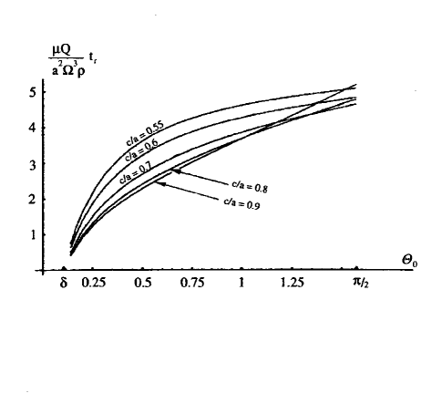
FIG. 1.: Precession of an oblate body: relaxation time $\,t_{r}\,$ as a function of $\,\theta_{0}\,$, where $\,\theta_{0}\,$ is the initial value of the precession-cone half-angle $\,\theta\,$. Precession begins with the precession-cone half-angle $\,\theta\,$ equal to $\,\theta_{0}\,$, and effectively ends when $\,\theta\,$ reaches the minimal measurable value $\;\delta\;$. On this plot, it is assumed that the initial value $\,\theta_{0}\,$ varies from $\;\delta\,=\,6^{0}\;$ through $\;\pi/2\;$. This choice of $\;\delta\;$ corresponds to the current abilities of ground-based radars. (Spacecraft-based instruments provide $\;\delta\,=\,0.01^{o}\;.$)

radars have a much sharper resolution and can grasp asteroid-shape details as fine as $\;10\;m\;$. This technique may reveal precession at half-angles of about 5 degrees. NEAR-type missions potentially may provide an accuracy of $\,0.01^{o}\;$ (Miller et al. 1999). For a time being, we would lean to a conservative estimate

$$\delta\;=\;6^{o}\;\;\;\;,\;\;\;$$ (54)

though we hope that within the coming years this limit may be reduced by three orders due to advances in the spacecraft-borne instruments.

Together, (48), (52) - (54) yield dependences illustrated by Fig.1. Remarkably, $\;t_{r}\;$ is not particularly sensitive to the half-sizes’ ratio $\;c/a\;$ when this ratio is between 0.5 - 0.9 (which is the case for realistic asteroids, comets and many spacecraft). Our formulae give:

$$t_{(our\;result)}\;\approx\;(1\;-\;2)\;\frac{\mu\;Q}{\rho\;a^{2}\;\Omega^{3}_{0}}\;\;\;\;\;\;for\;\;\;\;\;\;\theta_{0}\,\approx\,(2\;-\;3)\,\delta\;=\;12\;-\;18^{o}\;\;\;\;\;\;;$$ (55)

$$t_{(our\;result)}\;\approx\;(3\;-\;4)\;\frac{\mu\;Q}{\rho\;a^{2}\;\Omega^{3}_{0}}\;\;\;\;\;\;for\;\;\;\;\;\;\theta_{0}\,\approx\,\pi/4\;\;\;\;\;\;\;\;;\;\;\;\;$$ (56)

$$t_{(our\;result)}\;\approx\;(4\;-\;5)\;\frac{\mu\;Q}{\rho\;a^{2}\;\Omega^{3}_{0}}\;\;\;\;\;\;for\;\;\;\;\;\;\theta_{0}\,\stackrel{{\scriptstyle<}}{{\sim}}\,\pi/2\;\;\;\;\;\;.\;\;\;\;$$ (57)

(Mind though that, according to (51), $\theta$ should not approach $\pi/2$ too close.) To compare our results with a preceding study, recall that according to Burns & Safronov (1973)

$$t_{(B\;\&\;S)}\;\approx\;100\;\frac{\mu\;Q}{\rho\;a^{2}\;\Omega^{3}_{0}}\;\;\;.\;\;\;$$ (58)

The numerical factor in Burns & Safronov’s formula is about $100$ for objects of small oblateness, i.e., for comets and for many asteroids. (For objects of irregular shapes Burns and Safronov suggested a factor of about $\,20$ in place of $\,100$.)

This numerical factor is the only difference between our formula and that of Burns & Safronov. This difference, however, is quite considerable: for small residual half-angles $\;\theta\;$, our value of the relaxation time is two orders smaller than that predicted by Burns & Safronov. For larger residual half-angles, the times differ by a factor of several dozens. We see that the effectiveness of the inelastic relaxation was much underestimated by our predecessors. There are three reasons for this underestimation. The first reason is that our calculation was based on an improved solution to the boundary-value problem for stresses. Expressions (40) - (43) show that an overwhelming share of the deformation (and, therefore, of the inelastic dissipation) is taking place in the depth of the body. This is very counterintuitive, because on a heuristic level the picture of precession would look like this: a centrifugal bulge, with its associated strains, wobbles back and forth relative to the body as $\;\Omega\;$ moves through the body during the precession period. This naive illustration would make one think that most of the dissipation is taking place in the shallow regions under and around the bulge. It turns out that in reality most part of the deformation and dissipation takes place deep beneath the bulge (much like in the simple example with the liquid planet, that we provided in the end of section IV). The second, most important, reason for our formulae giving smaller values for the relaxation time is that we have taken into account the second harmonic. In many rotational states this harmonic turns to be a provider of the main share of the entire effect. In the expression $\;(63(c/a)^{4}\,\cot^{2}\theta+20)\;$ that is a part of formula (48), the term $\;63(c/a)^{4}\,\cot^{2}\theta\;$ is due to the principal frequency, while the term $\;20\;$ is due to the second harmonic. For $\;c/a\;$ belonging to the realistic interval $\;0.5\,-\,0.9\;$, the second harmonic contributes (after integration from $\;\theta_{0}\;$ through $\;\delta\;$) a considerable input in the entire effect. This input will be of the leading order, provided the initial half-angle $\;\theta_{0}\;$ is not too small (not smaller than about $\,30^{o}\,$). In the case of a small initial half-angle, the contribution of the second mode is irrelevant. Nevertheless it is the small-angle case where the discrepancy between our formula and (58) becomes maximal. The estimate (58) for the characteristic time of relaxation was obtained in Burns & Safronov (1973) simply as a reciprocal to their estimate for $\;\dot{\theta}\;$; it ignores any dependence upon the initial angle, and thus gives too long times for small angles. The dependence of the dissipation rate of the values of $\;\theta\;$ is the third of the reasons for our results being so different from the early estimate (58).

Exploration of this, third, reason may give us an important handle on observation of asteroid relaxation. It follows from (48) that a small decrease in the precession-cone half-angle, $\;-\,\Delta\theta\;$, will be performed during the following period of time:

$$\Delta t\;=\;(-\,\Delta\theta)\;\frac{2^{4}}{3}\;\frac{[1+(c/a)^{2}]^{4}}{63\;(c/a)^{4}\;\cot^{2}\theta\;+\;20}\;\frac{1}{\sin^{3}\theta}\;\frac{\mu\;Q}{a^{2}\;\Omega^{3}_{0}\;\rho}\;\;\;.$$ (59)

For asteroids composed of solid silicate rock, the density may be assumed $\;\rho\,\approx\,2.5\,\times\,10^{3}\;kg/m^{3}\;$, while the product in the numerator should be $\;\mu\,Q\,\approx\,1.5\,\times\,10^{13}\;dyne/cm^{2}\,=\,1.5\,\times\,10^{12}\,Pa\;$ as explained in Efroimsky & Lazarian (2000). Burns & Safronov suggested a much higher value of $\;3\,\times\,10^{14}\;dyne/cm^{2}\,=\,3\,\times\,10^{13}\,Pa\;$, value acceptable within the terrestial seismology but, probably, inapplicable to asteroids.

For asteroids composed of friable materials, Harris (1994) suggests the following values: $\;\rho\,\approx\,2\,\times\,10^{3}\;kg/m^{3}\;$ and $\;\mu\,Q\,\approx\,5\,\times\,10^{12}\;dyne/cm^{2}\,=\,5\,\times\,10^{11}\,Pa\;$. Naturally, this value is lower than those appropriate for solid rock (Efroimsky & Lazarian 2000), but in our opinion it is still too high for a friable medium. Harris borrowed the aforequoted value from preceding studies of Phobos (Yoder 1992). Mind, though, that Phobos may consist not only of rubble: it may have a solid component in the centre. In this case, a purely rubble-pile asteroid may have a lower $\;\mu\,Q\;$ than suggested by Harris. Anyway, as a very conservative estimate for a rubble-pile asteroid, we shall take the value suggested by Harris.

As for the geometry, let, for example, $\;\theta\,=\,\pi/3\;$ and $\;c/a\,=\,0.6\;$. Then

$$\Delta t\;=\;(-\,\Delta\theta)\;1.2\;\frac{\mu\;Q}{a^{2}\;\Omega^{3}_{0}\;\rho}\;\;\;.$$ (60)

If we measure time $\;\Delta t\;$ in years, the revolution period $\;T\,=\,2\,\pi/\Omega_{0}\;$ in hours, the maximal half-size $\;a\;$ in kilometers, and $\;\theta\;$ in angular degrees ($\Delta\theta\,=\,\Delta\theta^{o}\,\times\,1.75\,\times\,10^{-2}$), our formula (59) will yield:

$$\Delta t_{(years)}\;=\;(-\,\Delta\theta^{o})\;\times\;1.31\;\times\;10^{-7}\;\frac{\mu\;Q}{\rho}\;\frac{T^{3}_{(hours)}}{a^{2}_{(km)}}\;=\;0.33\;\frac{T^{3}_{(hours)}}{a^{2}_{(km)}}\;\;\;,$$ (61)

where we accepted Harris’ values of $\;\mu\,Q\,=\,5\,\times\,10^{11}\,Pa\;$ and $\rho\,=\,2\,\times\,10^{3}\;kg/m^{3}\;$, and the angular resolution of spacecraft-based devices was assumed to be as sharp as $\;|\Delta\theta|\,=\,0.01^{o}\;$, according to Miller et al. (1999).

VI Triaxial and prolate rotators

Typically, asteroids and comets have elongated shapes, and the above formulae derived for oblate bodies make a very crude approximation of the wobble of a triaxial or prolate body. In the case of a triaxial rotator, with $\;I_{3}\geq I_{2}\geq I_{1}\;$, the solution to the Euler equations is expressable in terms of elliptic functions. According to Jacobi (1882) and Legendre (1837), it will read, for $\;{\bf{J}}^{2}\;<\;2\;I_{2}\;T_{{kin}}\;$, as

$$\Omega_{1}\;=\;\gamma\;\,{\it{dn}}\left(\omega t,\;k^{2}\right)\;\;,\;\;\;\;\Omega_{2}\;=\;\beta\,\;\mathit{sn}\left(\omega t,\;k^{2}\right)\;\;,\;\;\;\;\Omega_{3}\;=\;\alpha\;\,{\it{cn}}\left(\omega t,\;k^{2}\right)\;\;,\;\;\;$$ (62)

while for $\;\;{\bf{J}}^{2}\;>\;2\;I_{2}\;T_{{kin}}\;$ it will be:

$$\Omega_{1}\;=\;{\gamma}\;\,{\it{cn}}\left({\omega}t,\;{k}^{2}\right)\;\;,\;\;\;\;\Omega_{2}\;=\;{\beta}\,\;{\it sn}\left({\omega}t,\;{k}^{2}\right)\;\;,\;\;\;\;\Omega_{3}\;=\;{\alpha}\;\,{\it{dn}}\left({\omega}t,\;{k}^{2}\right)\;\;.\;\;\;$$ (63)

Here the precession rate $\,\omega\,$ and the parameters $\;\alpha,\;\beta,\;\gamma\,$ and $\;{k}\;$ are some algebraic functions of $\;I_{1,2,3},\;T_{{kin}}\;$ and $\;{\bf J}^{2}\;$. For example, $\;{k}\;$ is expressed by

$$k\;=\;\sqrt{\frac{I_{3}-I_{2}}{I_{2}-I_{1}}\;\frac{{\bf J}^{2}-2I_{1}T_{kin}}{2I_{3}T_{kin}-{\bf J}^{2}}}\;\;\;\;\;,\;\;\;\;$$ (64)

for (62), and by

$$k\;=\;\sqrt{\frac{I_{2}-I_{1}}{I_{3}-I_{2}}\;\frac{2I_{3}T_{kin}-{\bf J}^{2}}{{\bf J}^{2}-2I_{1}T_{kin}}}\;\;\;\;\;,\;\;\;\;$$ (65)

for (63). In the limit of oblate symmetry (when $\;I_{2}/I_{1}\,\rightarrow\,1\;$), solution (63) approaches (25), while the applicability region of (62) shrinks. Similarly, in the prolate-symmetry limit ($\,(I_{3}\,-\,I_{2})/I_{1}\,\rightarrow\,0\,$) the applicability realm of (63) will become infinitesimally small. The easiest way of understanding this would be to consider, in the space $\;\Omega_{1}\;,\;\Omega_{2}\;,\;\Omega_{3}\;,$ the angular-momentum ellipsoid $\;\;{\bf{J}}^{2}\;=\;I_{1}^{2}\;\Omega_{1}^{2}\;+\;I_{2}^{2}\;\Omega_{2}^{2}\;+\;I_{3}^{2}\;\Omega_{3}^{2}\;\;$. A trajectory described by the angular-velocity vector $\;\bf\Omega\;$ in the space $\;\Omega_{1}\;,\;\Omega_{2}\;,\;\Omega_{3}\;$ will be given by a line along which this ellipsoid intersects the kinetic-energy ellipsoid $\;\;2\;T_{{kin}}\;=\;I_{1}\;\Omega_{1}^{2}\;+\;I_{2}\;\Omega_{2}^{2}\;+\;I_{3}\;\Omega_{3}^{2}\;\;,$ as on Fig.2. Through the relaxation process, the angular-momentum ellipsoid remains unchanged, while the kinetic-energy ellipsoid evolves as the energy dissipates. Thus, the fast process, precession, will be illustrated by the (adiabatically) periodic motion of $\;\bf\Omega\;$ along the line of ellipsoids’ intersection; the slow process, relaxation, will be illustrated by the gradual shift of the moving vector $\;\bf\Omega\;$ from one trajectory to another (Lamy & Burns 1972). On Fig.2, we present an angular-momentum ellipsoid for an almost prolate body whose angular momenta relate to one another as those of asteroid 433 Eros: $\;1\;\times\;3\;\times\;3.05\;$ (Black et al. 1999). Suppose the initial energy was so high that $\;\bf\Omega\;$ was moving along some trajectory close to the pole A on Fig.2. This pole corresponds to rotation of the body about its minor-inertia axis. The trajectory described by $\;\bf\Omega\;$ about $\,A\,$ is almost circular and remains so until $\;\bf\Omega\;$ approaches the separatrix. This process will be described by solution (62). In the vicinity of separatrix, trajectories will become noticeably distorted.

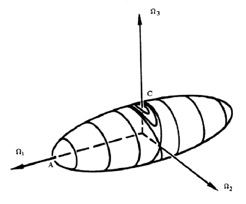
FIG. 2.: The constant-angular-momentum ellipsoid, in the angular-velocity space. The lines on its surface are its intersections with the kinetic-energy ellipsoids corresponding to different values of the rotational energy. The quasi-stable pole A is the maximal-energy configuration, i.e., the state when the body spins about its minimal-inertia axis. The stable pole C symbolises the minimal-energy state, i.e., rotation about the maximal-inertia axis. The angular-velocity vector precesses along the constant-energy lines, and at the same time slowly shifts from one line to another, approaching pole C. The picture illustrates the case of an elongated body: $I_{3}\stackrel{{\scriptstyle>}}{{\sim}}I_{2}>I_{1}$. The trajectories are circular near A and (in the case of an elongated body) remain virtually circular almost up to the separatrix. After the separatrix is crossed (with chaotic flipovers possible), the body starts tumbling. The trajectories will regain a circular shape only in the closemost proximity of C.

Crossing of the separatrix may be accompanied by stochastic flipovers. After the separatrix is crossed, librations will begin: $\;\bf\Omega\;$ will be describing not an almost circular cone but an elliptic one. This process will be governed by solution (63). Eventually, in the closemost vicinity of pole C, the precession will again become almost circular. (This pole, though, will never be reached because the alignment of $\;{\bf{\Omega}}\;$ towards $\;{\bf{J}}\;$ has a vanishing rate for small residual angles.) Parameter $\;k\;$ shows how far the tip of $\;\bf{\Omega}\;$ is from the separatrix on Fig.2: $\;k\;$ is zero in poles A and C, and is unity on the separatrix. It is defined by (64) when $\,\bf\Omega\,$ is between pole A and the separatrix, and by (65) when $\,\bf\Omega\,$ is between the separatrix and pole C. (For details see (Efroimsky 2000).)

If in the early stage of relaxation of an almost prolate ($I_{3}\,\approx\,I_{2}$) body the tip of vector $\;\bf{\Omega}\;$ is near pole A, then its slow departure away from A is governed by formula (9.22) in (Efroimsky 2000):

$$\frac{d\,\left\langle\sin^{2}\theta\right\rangle}{dt}\,=$$ (66)

(67)

$$-\,\frac{4\;\rho^{2}\;{\bf J}^{2}}{\mu\;Q(\omega)}\;\left(I_{3}\,-\,I_{1}\right)\;\left(1\,-\;\left\langle\sin^{2}\theta\right\rangle\,\right)\;\left\{\,\omega\,S_{1}\,\left[2\;\left\langle\sin^{2}\theta\right\rangle\;-\;1\;-\right.\right.$$ (68)

(69)

$$\left.\left.-\;\frac{1}{2}\;\frac{I_{3}\,-\,I_{2}}{I_{2}\,-\,I_{1}}\;\frac{I_{1}}{I_{3}}\;\left(1\,-\;\left\langle\sin^{2}\theta\right\rangle\,\right)\right]\;-\right.$$ (70)

(71)

$$\left.-\;\omega\;S_{0}\;\frac{2\,I_{1}}{I_{3}}\;\left(1\,-\;\left\langle\sin^{2}\theta\right\rangle\,\right)\;+\;2\,\omega\,S_{2}\;\frac{Q(2\omega)}{Q(\omega)}\;\frac{2\,I_{1}}{I_{3}}\;\left(1\,-\;\left\langle\sin^{2}\theta\right\rangle\,\right)\right\}\;.\;\;$$ (72)

where

$$\omega\;=\;\sqrt{\frac{\left(2\;I_{3}\;T_{{kin}}\;-\;{\bf{J}}^{2}\right)\;\left(I_{2}\;-\;I_{1}\right)}{I_{1}\;I_{2}\;I_{3}}}\;\approx\;\frac{|{\bf{J}}|}{I_{1}}\;\sqrt{\frac{\left(I_{3}\;-\;I_{1}\right)\;\left(I_{2}\;-\;I_{1}\right)}{I_{2}\;I_{3}}}\;\sqrt{2\;\left\langle\sin^{2}\theta\right\rangle\;-\;1}\;\;,\;\;$$ (73)

$\theta\;$ is the angle between the angular-momentum vector $\bf J$ and the major-inertia axis $\bf{3}\;\,$; $\;S_{0,1,2}$ are some geometrical factors ($S_{0}\,=\,0\,$ in the case of $\,I_{2}\,=\,I_{3}\,$), and $\;<...>\;$ symbolises an average over the precession cycle. For $\;<cos^{2}\theta>\;$ not exceeding $\;\approx\,1/7\;$, this equation has an exponentially decaying solution. For $\;c/a\,=\,0.6\;$ that solution will read:

$$\Delta t\;\approx\;(-\,\Delta\left\langle{\theta}\right\rangle)\;\times\;0.08\;\frac{\mu\;Q}{a^{2}\;\Omega^{3}_{0}\;\rho}\;\;\;.$$ (74)

Comparing this with (60), we see that at this stage the relaxation is about 15 times faster than in the case of an oblate body.

During the later stage, when $\bf{\Omega}$ gets close to the separatrix, all the higher harmonics will come into play, and our estimate will become invalid. How do the higher harmonics emerge? Plugging of (62) or (63) into (39) will give an expression for the acceleration of an arbitrary point inside the body. Due to (18), that expression will yield formulae for the stresses. These formulae will be similar to (40 - 43), but will contain elliptic functions instead of the trigonometric functions. In order to plug these formulae for $\;\sigma_{ij}\;$ into (22), they must first be squared and averaged over the precession cycle. For a rectangular prizm $\;2a\,\times\,2b\,\times\,2c\;$, a direct calculation performed in (Efroimsky 2000) gives:

$$\left\langle\sigma_{xx}^{2}\right\rangle=\frac{\rho^{2}}{4}\,(1-Q)^{2}\,\beta^{4}\,(x^{2}-a^{2})^{2}\;\Xi_{1}\;\;,\;\;\;\;$$ (75)

$$\left\langle\sigma_{yy}^{2}\right\rangle=\frac{\rho^{2}}{4}\,(S+Q)^{2}\,\beta^{4}\,(y^{2}-b^{2})^{2}\;\Xi_{1}\;\;\;,\;\;\;\;$$ (76)

$$\left\langle\sigma_{zz}^{2}\right\rangle=\frac{\rho^{2}}{4}\,(1-S)^{2}\,\beta^{4}\,(z^{2}-c^{2})^{2}\;\Xi_{1}\;\;\;,\;\;\;\;$$ (77)

$$\left\langle(Tr\,\sigma)^{2}\right\rangle=\frac{\rho^{2}}{4}\,\beta^{4}\,\left\{(1-Q)(x^{2}-a^{2})^{2}\,+\,(S+Q)(y^{2}-b^{2})\;+\;(1-S)(z^{2}-c^{2})\right\}^{2}\;\Xi_{1}\;\;\;,\;\;\;\;$$ (78)

$$\left\langle\sigma_{xy}^{2}\right\rangle=\frac{\rho^{2}}{4}\,\left\{(\beta\gamma+\alpha\omega k^{2})(y^{2}-b^{2})+(\beta\gamma-\alpha\omega k^{2})(x^{2}-a^{2})\right\}^{2}\;\Xi_{2}\;\;\;,\;\;\;\;$$ (79)

$$\left\langle\sigma_{xz}^{2}\right\rangle=\frac{\rho^{2}}{4}\,\left\{(\beta\omega+\alpha\gamma)(z^{2}-c^{2})+(\beta\omega-\alpha\gamma)(x^{2}-a^{2})\right\}^{2}\;\Xi_{3}\;\;\;,\;\;\;\;$$ (80)

$$\left\langle\sigma_{yz}^{2}\right\rangle=\frac{\rho^{2}}{4}\,\left\{(\alpha\beta+\omega\gamma)(z^{2}-c^{2})+(\alpha\beta-\omega\gamma)(y^{2}-b^{2})\right\}^{2}\;\Xi_{4}\;\;\;,\;\;\;\;$$ (81)

where $Q$ and $S$ are some combinations of $\,I_{1},\,I_{2},\,I_{3}\,$, defined by formula (2.8) in (Efroimsky 2000). Factors $\,\Xi_{1,2,3,4}\,$ stand for averaged powers of the elliptic functions:

$$\Xi_{1}\;\equiv\;\left\langle\,\;\left(\,{\it sn}^{2}(u,\,k^{2})\;-\;\,<\,{\it sn}^{2}(u,\,k^{2})\,>\,\;\right)^{2}\,\;\right\rangle\;=$$ (82)

(83)

$$=\;<\,{\it sn}^{4}(u,\,k^{2})\,>\;-\;<\,{\it sn}^{2}(u,\,k^{2})\,>^{2}\;\;\;,\;\;\;$$ (84)

$$\Xi_{2}\;\equiv\;\left\langle\,\;\left(\,\mathit{sn}(u,\,k^{2})\;\mathit{cn}(u,\,k^{2})\;-\;\left\langle\,\;\mathit{sn}(u,\,k^{2})\;\mathit{cn}(u,\,k^{2})\,\right\rangle\,\right)^{2}\,\;\right\rangle\;=$$ (85)

(86)

$$=\;<\,{\mathit{sn}}^{2}(u,\,k^{2})\;{\mathit{cn}}^{2}(u,\,k^{2})\,>\;-\;<\,\mathit{sn}(u,\,k^{2})\;\mathit{cn}(u,\,k^{2})\,>^{2}\;\;\;,\;\;\;$$ (87)

$$\Xi_{3}\;\equiv\;\left\langle\,\;\left(\;{\it cn}(u,\,k^{2})\;{\it dn}(u,\,k^{2})\;-\;\left\langle\,\;{\it cn}(u,\,k^{2})\;{\it dn}(u,\,k^{2})\,\;\right\rangle\,\;\right)^{2}\,\;\right\rangle\;=$$ (88)

(89)

$$=\;<\,{\it cn}^{2}(u,\,k^{2})\;{\it dn}^{2}(u,\,k^{2})\,>\;-\;<\,{\it cn}(u,\,k^{2})\;{\it dn}(u,\,k^{2})\,>^{2}\;\;\;,\;\;\;$$ (90)

(91)

$$\Xi_{4}\;\equiv\;\left\langle\,\;\left(\,{\mathit{sn}}(u,\,k^{2})\;{\mathit{dn}}(u,\,k^{2})\;-\;\left\langle\,\;{\mathit{sn}}(u,\,k^{2})\;{\mathit{dn}}(u,\,k^{2})\,\right\rangle\,\;\right)^{2}\,\;\right\rangle\;=$$ (92)

(93)

$$=\;<\,{\mathit{sn}}^{2}(u,\,k^{2})\;{\mathit{dn}}^{2}(u,\,k^{2})\,>\;-\;<\,{\mathit{sn}}(u,\,k^{2})\;{\mathit{dn}}(u,\,k^{2})\,>^{2}\;\;\;,\;\;\;$$ (94)

(95)

where averaging implies:

$$<...>\;\equiv\;\frac{1}{\tau}\;\int_{0}^{\tau}\;\,.\,.\,.\,\;du\;\;\;,\;\;\;$$ (96)

$\tau\;$ being the mutual period of $\,\mathit{sn}\,$ and $\,\mathit{cn}\,$ and twice the period of $\;\mathit{dn}\,$:

$$\tau\;=\;4\;K(k^{2})\;\equiv\;4\;\int_{0}^{\pi/2}\;(1\,-\,k^{2}\,\sin^{2}\psi)^{-1/2}\;d\,\psi\;\;\;.$$ (97)

The origin of expressions (84 - 95) can be traced from formulae (8.4,  8.6 - 8.13) in (Efroimsky 2000). For example, expression (34), that gives acceleration of an arbitrary point inside the body, contains term $\;\mathit{sn}^{2}(\omega t,\,k^{2})\;$. (Indeed, one of the components of the angular velocity is proportional to $\,\mathit{sn}(...)\,$, while the centripetal part of the acceleration is a quadratic form of the angular-velocity components.) The term $\;\mathit{sn}^{2}(\omega t,\,k^{2})\;$ in the formula for acceleration yields a similar term in the expression for $\;\sigma_{xx}\;$. For this reason expression (8.6) in (Efroimsky 2000), that gives the  time-dependent part of $\;\sigma_{xx}\;$, contains $\;\mathit{sn}^{2}(...)\,-\,<sn^{2}(...)>\;$, wherefrom (84) ensues.

Now imagine that in the formulae (75 - 81) the elliptic functions are presented by their series expansions over sines and cosines (Abramovitz & Stegun 1965):

$${\mathit{sn}}(\omega t,\,k^{2})\;=\;\frac{2\pi}{k\,K}\sum_{n=1}^{\;\;\;\;\;\infty\;\;\;*}\frac{q^{n/2}}{1\,-\,q^{n}}\;\sin\left(\omega_{n}\,t\right)\;\;\;\;\;,\;\;\;\;\;$$ (98)

$${\mathit{cn}}(\omega t,\,k^{2})\;=\;\frac{2\pi}{k\,K}\sum_{n=1}^{\;\;\;\;\;\infty\;\;\;*}\frac{q^{n/2}}{1\,+\,q^{n}}\;\cos\left(\omega_{n}\,t\right)\;\;\;\;\;,\;\;\;\;\;$$ (99)

$${\mathit{dn}}(\omega t,\,k^{2})\;=\;\frac{\pi}{2\,K}\;+\;\frac{2\pi}{K}{\sum_{n=0}^{\;\;\;\;\;\infty\;\;\;**}}\;\frac{q^{{n}/{2}}}{1\,+\,q^{n}}\;\cos\left(\omega_{n}\,t\right)\;\;\;\;\;,\;\;\;\;\;$$ (100)

where

$$\omega_{n}\,=\,n\,\omega\,\pi/(2K(k^{2}))\;\;\;,\;\;\;q\,=\,\exp(-\pi K({k^{\prime}}^{2})/K(k^{2}))\;\;\;,\;\;\;{k^{\prime}\,}^{2}\,\equiv\,1\,-\,k^{2}\;\;$$ (101)

and the function $\,K(k^{2})\,$ is the complete elliptic integral of the first kind (see (97) or (108)). A star in the superscript denotes a sum over odd $n$’s only; a double star stands for a sum over even $n$’s. Plugging of (98-100) into (75-81) will produce, after squaring of $\;\mathit{sn},\,\mathit{cn},\,\mathit{dn}\;$, an infinite amount of terms like $\;\sin^{2}(\omega_{n}t)\;$ and $\;\cos^{2}(\omega_{n}t)\;$, along with an infinite amount of cross terms. The latter will be removed after averaging over the precession period, while the former will survive for all $n$’s and will average to 1/2. Integration over the volume will then lead to an expression like (14), with an infinite amount of contributions $\;\left\langle W_{n}\right\rangle\;$ originating from all $\,\omega_{n}\,$’s, $\;n\,=\,1,\,.\,.\,.\,,\,\infty$. This is how an infinite amount of overtones comes into play. These overtones are multiples not of precession rate $\,\omega\,$ but of the ”base frequency” $\,\omega_{1}\,\equiv\,\omega\pi/(2K(k^{2}))\,$ which is lower than $\,\omega\,$. Hence the stresses and strains contain not only Fourier components oscillating at frequencies higher than the precession rate, but also components oscillating at frequencies lower than $\,\omega\,$. This is a very unusual and counterintuitive phenomenon.

The above series (called ”nome expansions”) typically converge very quickly, for $\,q\,\ll\,1\,$. Note, however, that $\,q\,\rightarrow\,1\,$ at the separatrix. Indeed, on approach to the separatrix we have: $\,k\,\rightarrow\,1\,$, wherefrom $\,K(k^{2})\,\rightarrow\,\infty\,$; therefore $\,q\,\rightarrow\,1\,$ and $\,\omega_{n}\,\rightarrow\,0\,$ (see eqn. (101)). The period of rotation (see (97)) becomes infinite. (This is the reason why near-separatrix states can mimic the principal one.)

Our previous work, Efroimsky (2000), addressed relaxation in the vicinity of poles. This case corresponds to $\;k\,\ll\,1\,$. For this reason we used, instead of (98 - 100), trivial approximations $\;\omega_{1}\,\approx\,\omega\;,\;\mathit{sn}(\omega t,\,k^{2})\,\approx\,\sin(\omega t)\;,\;\mathit{cn}(\omega t,\,k^{2})\,\approx\,\cos(\omega t)\;,\;\mathit{dn}(\omega t,\,k^{2})\,\approx\,$1. These approximations, along with (75 - 95) enabled us to assume that the terms $\,\sigma_{xz}^{2}\,$ and $\,\sigma_{yz}^{2}\,$ in (29) are associated with the principal frequency $\,\omega\,$, while $\,<\sigma_{xx}^{2}>\,$, $\,<\sigma_{yy}^{2}>\,$, $\,<\sigma_{zz}^{2}>\,$, $\,<(Tr\,\sigma)^{2}>\,$ and $\,\sigma_{xy}^{2}\,$ are associated with the second harmonic $\;2\,\omega\,$. No harmonics higher than second appeared in that case. However, if we move away from the poles, parameter $\,k\,$ will no longer be small (and will be approaching unity as we approach the separatrix). Hence we shall have to take into account all terms in (98 - 100) and, as a result, shall get an infinite amount of contributions from all $\;\omega_{n}\,$’s in (22 - 14). Thus we see that the problem is very highly nonlinear. It is nonlinear even though the properties of the material are assumed linear (strains $\;\epsilon\;$ are linear functions of stresses $\;\sigma\;$). Retrospectively, the nonlinearity originates because the dissipation rate (and, therefore, the relaxation rate) is proportional to the averaged (over the cycle) elastic energy stored in the body experiencing precession-caused alternating deformations. The average elastic energy is proportional to $\;<\sigma\,\epsilon>\;$, i.e., to $\;<\sigma^{2}>\;$. The stresses are proportional to the components of the acceleration, that are quadratic in the components of the angular velocity (62 - 63). All in all, the relaxation rate is a quartic form of the angular-velocity components that are expressed by the elliptic functions $\;(\ref{6.16}-\ref{6.18})\;$.

A remarkable fact about this nonlinearity is that it produces oscillations of stresses and strains not only at frequencies higher than the precession frequency $\;\omega\;$ but also at frequencies lower than $\,\omega$. This is evident from formula (101): the closer we get to the separatrix (i.e., the closer $\,k^{2}\,$ gets to unity), the smaller the factor $\;\pi/(2K)\;$, and the more lower-than-$\omega$ frequencies emerge.

A quantitative study of near-separatrix wobble will imply attributing extra factors of $\;\omega_{n}/Q(\omega_{n})\;$ to each term of the series (14) and investigating the behaviour of the resulting series (15). This study will become the topic of our next paper. Nevertheless, some qualitative judgement about the near-separatrix behaviour can be made even at this point.

For the calculation of the dissipation rate (15), the value of the average elastic energy $\,<W>\,$ given by the sum (14) is of no use (unless each of its terms is multiplied by $\;\omega_{n}/Q(\omega_{n})\;$ and plugged into (15)). For this reason, the values of the terms $\,<\sigma_{ij}^{2}>\,$ entering (22) are of no practical value either; only their expansions obtained by plugging (98 - 100) into (75 - 95) do matter. Nonetheless, let us evaluate $\,<W>\,$ near the separatrix. To that end, one has to calculate all $\,<\sigma_{ij}^{2}>\,$’s by evaluating (84 - 95). Direct integration in (84 - 96) leads to:

$$\Xi_{1}\;=\;\frac{1}{3\,k^{4}}\;\left\{k^{2}\;-\;1\;+\;\frac{2\,E}{K}\;\left(2\,-\,k^{2}\right)\;-\;3\;\left(\frac{E}{K}\right)^{2}\right\}\;\;\;\;,\;\;\;$$ (102)

$$\Xi_{2}\;=\;\frac{1}{3\,k^{4}}\;\left\{2\;\left(k^{2}\;-\;1\right)\;+\;\frac{E}{K}\;\left(\,-\,2\,-\,5\,k^{2}\right)\right\}\;\;\;\;,\;\;\;$$ (103)

$$\Xi_{3}\;=\;\frac{1}{3\,k^{2}}\;\left\{\frac{E}{K}\;\left(1\;+\;k^{2}\right)\;+\;\left(k^{2}\;-\;1\right)\right\}\;\;\;\;,\;\;\;$$ (104)

(105)

$$\Xi_{4}\;=\;\frac{1}{3\,k^{2}}\;\left\{\frac{E}{K}\;\left(2\;k^{2}\;-\;1\right)\;+\;\left(1\;-\;k^{2}\right)\right\}\;\;\;\;,\;\;\;$$ (106)

$K\,$ and $\;E\;$ being abbreviations for the complete elliptic integrals of the 1st and 2nd kind:

$$K\;\equiv\;K(k^{2})\;\equiv\;\int_{0}^{\pi/2}\;(1\,-\,k^{2}\,\sin^{2}\psi)^{-1/2}\;d\,\psi\;\;\;,$$ (107)

(108)

$$E\;\equiv\;E(k^{2})\;\equiv\;\int_{0}^{\pi/2}\;(1\,-\,k^{2}\,\sin^{2}\psi)^{1/2}\;d\,\psi\;\;\;.\;\;\;$$ (109)

In the limit of $\,k\,\rightarrow\,1\,$, the expression for $\;K\;$ will diverge and all $\;\Xi_{i}\;$ will vanish. Then all $\,<\sigma_{ij}^{2}>\,$ will also become nil, and so will $\,<W>\,$. As all the inputs $\,<W(\omega_{n})>\,$ in (15) are nonnegative, each of them will vanish too. Hence the relaxation slows down near the separatrix. Moreover, it appears to completely halt on it. How trustworthy is this conclusion? On the one hand, it might have been guessed simply from looking at (97): since for $\,k\,\rightarrow\,1\,$ the period $\,4\,K(k^{2})\,$ diverges (or, stated differently, since the frequencies $\,\omega_{n}\,$ in (101) approach zero for each fixed n, then all the averages may vanish). On the other hand, though, the divergence of the period undermines the entire averaging procedure: for $\;\tau\;\rightarrow\;\infty\;$, expression (11) becomes pointless. Let us have a look at the expressions for the angular-velocity components near the separatrix. According to (Abramovits & Stegun 1965), these expressions may be expanded into series over small parameter $\;(1-k^{2})\;$:

$$\Omega_{1}\;=\;\gamma\;\,{\it{dn}}\left(\omega t,\;k^{2}\right)\;=\;\gamma\;\,\left\{{\it{sech}}\left(\omega t\right)^{\left.~{}\right.}_{\left.~{}\right.}\;+\right.\;\;\;\;\;\;\;\;\;\;\;\;\;\;\;$$ (110)

(111)

$$\left.+\;\frac{1}{4}\;(1\,-\,k^{2})\;\left[{\mathit{sinh}}(\omega t)\;{\mathit{cosh}}(\omega t)\;+\;\omega\,t\right]\;{\mathit{sech}}(\omega t)\;{\mathit{tanh}}(\omega t)\right\}\;+\;O\left((1-k^{2})^{2}\right)\;\;\;,\;\;$$ (112)

$$\Omega_{2}\;=\;\beta\,\;{\mathit{sn}}\left(\omega t,\;k^{2}\right)\;=\;\beta\;\,\left\{{\mathit{tanh}}^{\left.\right.}_{\left.\right.}(\omega t)\;+\;\right.\;\;\;\;\;\;\;\;\;\;$$ (113)

(114)

$$\left.+\;\frac{1}{4}\;(1\,-\,k^{2})\;\left[{\mathit{sinh}}(\omega t)\;{\mathit{cosh}}(\omega t)\;-\;\omega\,t\right]\;{\mathit{sech}}^{2}(\omega t)\right\}\;+\;O\left((1-k^{2})^{2}\right)\;\;\;,\;\;$$ (115)

$$\Omega_{3}\;=\;\alpha\;\,{\it{cn}}\left(\omega t,\;k^{2}\right)\;=\alpha\;\,\left\{{\mathit{sech}}(\omega t)\;-\;\right.\;\;\;\;\;\;\;\;\;\;$$ (116)

(117)

$$\left.-\;\frac{1}{4}\;(1\,-\,k^{2})\;\left[{\mathit{sinh}}(\omega t)\;{\mathit{cosh}}(\omega t)\;-\;\omega\,t\right]\;{\mathit{sech}}(\omega t)\;{\mathit{tanh}}(\omega t)\right\}\;+\;O\left((1-k^{2})^{2}\right)\;\;\;.\;\;$$ (118)

These expansions will remain valid for small $\;k^{2}\;$ up to the point $\;k^{2}\,=\,1\;$, inclusively. It doesn’t mean, however, that in these expansions we may take the limit of $\;t\,\rightarrow\,\infty\;$. (This difficulty arises because this limit is not necessarily interchangeable with the infinite sum of terms in the above expansions.) Fortunately, though, for $\;k^{2}\,=\,1\;$, the limit expressions

$$\Omega_{1}\;=\;\gamma\;\,{\it{dn}}\left(\omega t,\;1\right)\;=\;\gamma\;\,{\it{sech}}\left(\omega t\right)\;\;\;\;,\;\;$$ (119)

$$\Omega_{2}\;=\;\beta\,\;{\mathit{sn}}\left(\omega t,\;1\right)\;=\;\beta\;\,{\mathit{tanh}}(\omega t)\;\;\;\;,\;\;$$ (120)

$$\Omega_{3}\;=\;\alpha\;\,{\it{cn}}\left(\omega t,\;1\right)\;=\;\alpha\;\,{\mathit{sech}}(\omega t)\;\;\;\;\;\;$$ (121)

make an exact solution to (1). Thence we can see what happens to vector $\;\bf{\Omega}\;$ when its tip is right on the separatrix. If there were no inelastic dissipation, the tip of vector $\;\bf{\Omega}\;$ would be slowing down while moving along the separatrix, and will come to halt at one of the middle-inertia homoclinic unstable poles (though it would formally take $\;\bf{\Omega}\;$ an infinite time to get there, because $\,\Omega_{1}\,$ and $\,\Omega_{3}\,$ will be approaching zero as $\;\sim\,\exp(-\omega t)\;\,$). When $\;\bf{\Omega}\;$ gets sufficiently close to the homoclinic point, the precession will slow down so that an observer would get an impression that the body is in a simple-rotation state. In reality, some tiny dissipation will still be present even for very slowly evolving $\;\bf{\Omega}\;$. It will be present because this slow evolution will cause slow changes in the stresses and strains. The dissipation will result in a further decrease of the kinetic energy, that will lead to a change in the value of $\;k^{2}\;$ (which is a function of energy; see (64) and (65)). A deviation of $\;k^{2}\;$ away from unity will imply a shift of $\;\bf{\Omega}\;$ away from the separatrix towards pole C. So, the separatrix eventually will be crossed, and the near-separatrix slowing-down does NOT mean a complete halt.

This phenomenon of near-separatrix slowing-down (that we shall call lingering effect) is not new. In a slightly different context, it was mentioned by Chernous’ko (1968) who investigated free precession of a tank filled with viscous liquid and proved that, despite the apparent trap, the separatrix is crossed within a finite time. Recently, the capability of near-intermediate-axis rotational states to mimic simple rotation was pointed out by Samarasinha, Mueller & Belton (1999) with regard to comet Hale-Bopp.

We, thus, see that the near-separatrix dissipational dynamics is very subtle, from the mathematical viewpoint. On the one hand, more of the higher overtones of the base frequency will become relevant (though the base frequency itself will become lower, approaching zero as the angular-velocity vector approaches the separatrix). On the other hand, the separartrix will act as a (temporary) trap, and the duration of this lingering is yet to be estimated.

One should, though, always keep in mind that a relatively weak push can help the spinning body to cross the separatrix trap. So, for many rotators (at least, for the smallest ones, like cosmic-dust grains) the observational reality near separatrix will be defined not so much by the mathematical sophistries but rather by high-order physical effects: the solar wind, magnetic field effects, etc… In the case of a macroscopic rotator, a faint tidal interaction or a collision with a smaller body may help to cross the separatrix.

VII Application to Asteroids and Comets

Let us begin with 4179 Toutatis. This is an S-type asteroid analogous to stony irons or ordinary chondrites, so the solid-rock value of $\;\mu\,Q\;$ suggested in Efroimsky & Lazarian (2000) may be applicable to it: $\;\mu\,Q\,\approx\,1.5\,\times\,10^{13}\;dyne/cm^{2}\,=\,1.5\,\times\,10^{12}\,Pa\;$. Its density may be roughly estimated as $\;\rho\,=\,2.5\,\times\,10^{3}\;kg/m^{3}\;$ (Scheeres et al. 1998). Just as in the case of (61), let us measure the time $\;\Delta t\;$ in years, the revolution period $\;T\;$ in hours ($T_{(hours)}\,=\,175$), the maximal half-radius $\;a\;$ in kilometers ($\;a_{(km)}\,=\,2.2\;$), and $\;\theta\;$ in angular degrees ($|\Delta\theta^{o}|\,=\,0.01$). Then (74) will yield:

$$\Delta t_{(years)}\;\approx\;5.1\;\times\;10^{-2}\;\frac{T^{3}_{(hours)}}{a^{2}_{(km)}}\;=\;5.6\;\times\;10^{4}\;years$$ (122)

Presently, the angular-velocity vector $\,\bf\Omega\,$ of Toutatis is at the stage of precession about $\,A\;$ (see Fig.2). However its motion does not obey the restriction $\;{\left\langle\cos^{2}\theta\right\rangle}\,<\,1/7\,$ under which (74) works well. A laborious calculation based on equations (2.16) and (A4) from Efroimsky (2000) and on formulae (1), (2) and (11) from Scheeres et al (1998) shows that in the case of Toutatis $\;{\left\langle\cos^{2}\theta\right\rangle}\,\approx\,2/7\,$. Since the violation is not that bad, one may still use (122) as the zeroth approximation. Even if it is a two or three order of magnitude overestimate, we still see that the chances for experimental observation of Toutatis’ relaxation are slim.

This does not mean, though, that one would not be able to observe asteroid relaxation at all. The relaxation rate is sensitive to the parameters of the body (size and density) and to its mechanical properties ($\,\mu Q\,$), but the precession period is certainly the decisive factor. Suppose that some asteroid is loosely-connected ($\;\mu\,Q\,=\,5\,\times\,10^{12}\,dyne/cm^{2}\,=\,5\,\times\,10^{11}\,Pa\;$ and $\rho\,=\,2\,\times\,10^{3}\;kg/m^{3}\;$), has a maximal half-size 17 km, and is precessing with a period of 30 hours, and is not too close to the separatrix. Then an optical resolution of $|\Delta\theta^{o}|\,=\,0.01$ degrees will lead to the following time interval during which a $\;0.01^{o}\;$ change of the precession-cone half-angle will be measurable:

$$\Delta t_{(years)}\;\approx\;2.12\;\times\;10^{-2}\;\frac{T^{3}_{(hours)}}{a^{2}_{(km)}}\;=\;2\;\;years\;\;\;\;$$ (123)

which looks most encouraging. In real life, though, it may be hard to observe precession relaxation of an asteroid, for one simple reason: too few of them are in the states when the relaxation rate is fast enough. Since the relaxation rate is much faster than believed previously, most excited rotators have already relaxed towards their principle states and are describing very narrow residual cones, too narrow to observe. The rare exceptions are asteroids caught in the near-separatrix ”trap”. These are mimicing the principal state.

On these grounds, it is easy to guess the rotational state of 433 Eros: since it is not in a sweep-tumble mode, then most probably it is not precessing at all, or keeps an extremely narrow residual cone. An almost circular precession with a half-angle of several degrees is very improbable because most likely it has already been transcended. Indeed, the observations have indicated no visible wobble (Yeomans $\it{et\;al}$ 2000).

What about comets? According to Peale and Lissauer (1989), for Halley’s comet $\mu\approx 10^{10}\,dyne/cm^{2}\,=\,10^{9}\,Pa\,$ while $Q<100$, like for the regular ice. We are unsure if the values of order $\,100\,$ for $Q$ are acceptable; we would be more comfortable with values close to those of firn (heavy coarse-grained snow): $Q\approx 1$. Then $\mu Q\approx 10^{10}\,dyne/cm^{2}\,=\,10^{9}\,Pa$. As for the density of the cometary material, it is probable that the average density of a comet does not deviate much from $1.5\,\times\,10^{3}\,kg/m^{3}$. Indeed, on the one hand, the major part of the material may have density close to that of firn, but on the other hand a typical comet will carry a lot of crust and dust on and inside itself. Now, consider a comet of a maximal half-size 7.5 km (like that of Halley comet (Houpis and Gombosi 1986)) precessing with a period of 3.7 days $\approx$ 89 hours (just as Halley does). If we once again assume the angular resolution of the spacecraft-based equipment to be $|\Delta\theta^{o}|\,=\,0.01$, it will lead us to the following damping time:

$$\Delta t_{(years)}\;\approx\;5.65\;\times\;10^{-5}\;\frac{T^{3}_{(hours)}}{a^{2}_{(km)}}\;=\;0.7\;\;year\;\;\;.\;$$ (124)

This means that the cometary-relaxation damping may be measurable.

It also follows from (124) that, to maintain the observed tumbling state of the Comet P/Halley, its jet activity should be sufficiently high.

VIII Application to Asteroid 433 Eros in Light of Recent Observations

As already mentioned in the above section, asteroid 433 Eros is in a spin state that is either principal one or very close to it. This differs from the scenario studied in (Black et al 1999). According to that scenario, an almost prolate body would be spending most part of its history wobbling about the minimal-inertia axis. Such a scenario was suggested because the gap between the separatrices embracing pole C on Fig.2 is very narrow, for an almost prolate top, and therefore, a very weak tidal interaction or impact would push the asteroid’s angular velocity vector $\bf{\Omega}$ across the separatrix, away from pole C. This scenario becomes even more viable due to the ”lingering effect” described in section V, i.e., due to the relative slowing down of the relaxation in the closemost vicinity of the separatrix.

Nevertheless, this scenario has not been followed by Eros. This could have happened for one of the following reasons: either the dissipation rate in the asteroid is high enough to make Eros well relaxed after the recentmost disruption, or the asteroid simply has not experienced impacts or tidal interactions since times immemorial (since the early days of the Solar System, if we use the estimates by Burns & Safronov (1973) who argued that the characteristic times of asteroid relaxation may be of order hundred of millions to billion years).

The latter option is very unlikely: currently Eros is at the stage of leaving the main belt; it comes inside the orbit of Mars and approaches that of the Earth. It is then probable that Eros during its recent history was disturbed by the tidal forces that drove it out of the principal spin state.

Hence we have to prefer the former option, option that complies with our theory of precession relaxation. The fact that presently Eros is within less than 0.1 degree from its principal spin state means that the precession relaxation process is a very fast process, much faster than believed previously.

IX Unresolved issues

Our approach to calculation of the relaxation rate is not without its disadvantages. Some of these are of mostly aesthetic nature, but at least one is quite alarming.

As was emphasised in the end of Section II, our theory is adiabatic, in that it assumes the presence of two different time scales or, stated differently, the superposition of two motions: slow and fast. Namely, we assumed that the relaxation rate is much slower than the body-frame-related precession rate $\,\omega\,$ (see formulae (5) and (6)). This enabled us to conveniently substitute the dissipation rate by its average over a precession cycle. The adiabatic assertion is not necessarily fulfilled when $\,\omega\,$ itself becomes small. This happens, for example, when the dynamical oblateness of an oblate ($\,I_{3}\,>\,I_{2}\,=\,I_{1}\,\equiv\,I\,$) body is approaching zero:

$$(h\,-\,1)\,\rightarrow\,0\;\;\;,\;\;\;\;\;\;\;\;\;\;\;h\;\equiv\;I_{3}/I\;\;\;\;.\;\;\;$$ (125)

Since in the oblate case $\,\omega\,$ is proportional to the oblateness (see (5.4)), it too will approach zero, making our adiabatic calculation inapplicable. This is the reason why one cannot and shouldn’t compare our results, in the limit of $\,(h\,-\,1)\,\rightarrow\,0\,$, with the results obtained by Peale (1973) for an almost-spherical oblate body.

In the general, triaxial case, our result, should not be compared, in the limit of weak triaxiality, to those presented in Peale, Cassen & Reynolds (1979) and Yoder (1982), because those papers addressed not free dissipation but tidal dissipation. Our results, in the limit of weak triaxiality, should not be compared either to those obtained by Yoder & Ward (1979) for Venusian wobble-damping rate. The results of Yoder & Ward (1979) are correct in the limit they were designed for, i.e., for an almost spherical planet. None of the asteroids and comets are almost spherical; hence they are subject to our approach, not to that of Yoder & Ward.

Another minor issue, that has a lot of mathematics in it but hardly bears any physical significance, is our polynomial approximation (40 - 43  ,  75 - 81) to the stress tensor. As explained in Section V, this approximation keeps the symmetry $\,\sigma_{ij}\,=\,\sigma_{ji}\,$ and exactly satisfies (18) with (39) plugged in. The boundary conditions are fulfilled exactly for the diagonal components of the tensor and approximately for the off-diagonal elements. In the calculation of the relaxation rate, this approximation will result in some numerical factor, and it is highly improbable that this factor differs much from unity.

A more serious difficulty of our theory is that it cannot, without further refinement, give a reasonable estimate for the duration of the near-separatrix slowing-down mentioned in the end of Section VI. On the one hand, many (formally, infinitely many) overtones of the base frequency $\,\omega_{1}\,$ come into play near the separatrix; on the other hand, the base frequency approaches zero. Thence, it will take some extra work to account for the dissipation associated with the stresses oscillating at $\,\omega_{1}\,$ and with its lowest overtones. (The dissipation due to the stresses at these low frequency cannot be averaged over their periods.)

There exists, however, one more, primary difficulty of our theory. Even though our calculation predicts a much faster relaxation rate than believed previously, it still may fail to account for the observed relaxation which seems to be even faster than we expect. This paper was already in press when Andrew Cheng confirmed the preliminary conclusion of the NEAR team, that the upper limit on non-principal axis rotation is better than 0.1 angular degree. How to interpret such a tough observational limit on Eros’ residual precession-cone width? Our theory does predict very swift relaxation, but it also shows that the relaxation slows down near the separatrix and, especially, in the closemost vicinity of poles $\,A\,$ and $\,C\,$. Having arrived to the close vicinity of pole $\,C\,$, the angular-velocity vector $\,\Omega\,$ must exponentially slow down its further approach to $\,C\,$ (see the paragraph after equation (5.23)). For this reason, a body that is monolithic (so that its $\,\mu Q\,$ is not too low) and whose motion is sometimes influenced by tidal or other interactions, must demonstrate to us at least some narrow residual precession cone. As already mentioned, for the past million or several millions of years Eros has been at the stage of leaving the main belt. It comes inside the Mars orbit and approaches the Earth. It is possible that Eros experienced a tidal interaction within the said period of its history. Nevertheless it is presently in or extremely close to its principal spin state. The abscence of a visible residual precession not only disproves the old theory but also indicates that our new-born theory, too, may be incomplete. In particular, our $\,Q$-factor-based empirical description of attenuation should become the fair target for criticisms, because it ignores several important physical effects.

One such effect is material fatigue. It shows itself whenever a rigid material is subject to repetitive load. In the case of a wobbling asteroid or comet, the stresses are tiny, but the amount of repetitive cycles, accumulated over years, is huge. At each cycle, the picture of emerging stresses is virtually the same. Moreover, beside the periodic stresses, there exists a constant component of stress. This may lead to creation of ”weak points” in the material, points that eventually give birth to cracks or other defects. This may also lead to creep, even in very rigid materials. The creep will absorb some of the excessive energy associated with precession and will slightly alter the shape of the body. The alteration will be such that the spin state becomes closer to the one of minimal energy. It will be achieved through the slight change in the direction of the principal axes in the body. If this shape alteration is due to the emergence of a considerable crack or displacement, then the subsequent damping of precession will be performed by a finite step, not gradually.

Another potentially relevant phenomenon is the effect that a periodic forcing (such as the solar gravity gradient) would have on the evolution and relaxation of the precession dynamics. It is possible that this sort of forcing could influence the precessional dynamics of the body.

X Rubble heap versus monolith

Above we mentioned one of the most important discoveries of the NEAR-Schoemaker mission: Eros is a well-connected monolith. This brings up an interesting issue that is still unresolved.

At present, most astronomers lean toward the rubble-pile hypothesis, in regard to both asteroids and comets. The hypothesis originated in mid-sixties (${\ddot{O}}$pik 1966) and became a dominating theory in the end of the past century (Burns 1975; Asphaug & Benz 1994; Harris 1996; Asphaug & Benz 1996; Bottke & Melosh 1996a,b; Richardson, Bottke & Love 1998; Bottke 1998, Bottke, Richardson & Love 1998; Bottke, Richardson, Michel & Love 1999, Pravec & Harris 2000).

Sometimes comets get rent apart by the tidal forces (Asphaug & Benz 1996, Sekanina 1982, Melosh & Schenk 1993). On these and other grounds many researchers conclude that all comets are weakly connected. A possible counter argument may be the following: since the comets, when warmed up by the Sun, are prone to tidal disintegration, then perhaps, the weakest comets have already perished and only the strongest have survived. Hopefully, our understanding of the subject will improve after the Deep Impact mission reaches its goal. Meanwhile, we would lean towards the moderate viewpoint (Efroimsky & Lazarian 2000): at least some of the comets are loosely connected conglomerates, but we do not know if all or even if most of them are like that

In the case of asteroids, it may be unwise of us to completely reject the rubble-pile hypothesis. This hypothesis rests on several strong arguments the main of which is this: the large fast-rotating asteroids are near the rotational breakup limit for aggregates with no tensile strength. Still, we would object to two of the arguments often used in support this theory. One such dubious argument is the low density of asteroid 253 Mathilde. The low density of Mathilde (Veverka et al 1998, Yeomans et al 1998) may indeed evidence of high porosity. However, in our opinion, the word ”porous” is not necessarily a synonim to ”rubble-pile”, even though in the astronomical community they are often used as synonims. In fact, a material may have high porosity and, at the same time, be rigid.

Another popular argument, that we would contest, is the one about crator shapes. Many colleagues believe that a rigid body would be shattered into smitherines by collisions; therefrom they infer that the asteroids must be soft, i.e., rubble. In our opinion, though, a rigid but highly porous material may stand very energetic collisions without being destroyed, because its porous structure damps the impact.

Finally, it is know from the construction engineering that some materials, initially friable, become relatively rigid after being heated up (like, for example, asphalt). They remain porous and may be prone to creep, but they are, nevertheless, sufficently rigid and well connected.

For these three reasons, we expressed in Efroimsky & Lazarian (2000) our conservative opinion on the subject: at least some asteroids are well-connected solid chunks, though we are uncertain whether this is true for all asteroids. This opinion met a cold reaction from the community. However, it is supported by the recentmost findings. The monolithic nature of Eros is the most important of these. Other include 1998KY26 studied in 1999 by Steven Ostro and his team: from the radar and optical observations, the team inferred that this body, as well as several other objects, is monolithic (Ostro et al 1999).

Still, we have to admit that the main argument in favour of rubble-pile hypothesis (the absence of large fast rotators) remains valid.

XI conclusions

1. In many spin states, dissipation at frequencies different from the precession frequency makes a major input into the inelastic-relaxation process. These frequencies are overtones of some ”basic” frequency, that is LOWER than the precession frequency. Thereby we encounter a very unusual example of nonlinearity: the principal frequency (precession rate) gives birth not only to higher frequencies but also to lower frequencies.

2. Distribution of stresses and strains over the volume of a precessing body is such that a major share of inelastic dissipation is taking place deep inside the body, not in its shallow regions, as thought previously. These and other reasons make inelastic relaxation far more effective than believed hitherto.

3. However, if the rotation states that are close to the separatrix on Fig.2, the lingering effect takes place: both precession and precession-damping processes slow down. Such states (especially those close to the homoclinic point) may mimic the principal rotation state.

4. A finite resolution of radar-generated images puts a limit on our ability of recognising whether an object is precessing or not. Relaxation-caused changes of the precession-cone half-angle may be observed. Our estimates show that the modern spacecraft-based instruments are well fit for observations of the asteroid and cometary wobble relaxation. In many rotation states, relaxation may be registered within relatively short periods of time (about a year).

5. Measurements of the damping rate will provide us with valuable information on attenuation in small bodies, as well as on their recent histories of impacts and tidal interactions

6. Since inelastic relaxation is far more effective than presumed earlier, the number of asteroids expected to wobble with a recognisable half-angle of the precession cone must be lower than expected. (We mean the predictions suggested in (Harris 1994).) Besides, some of the small bodies may be in the near-separatrix states: due to the afore mentioned lingering effect, these rotators may be “pretending” to be in a simple rotation state.

7. Even though our theory predicts a much higher relaxation rate than believed previously, this high rate may still be not high enough to match the experimentally available data. In the closemost vicinity of the principal spin state the relaxation rate must decrease and the rotator must demonstrate the ”exponentially-slow finish”. Asteroid 433 Eros is a consolidated rotator whose $Q$-factor should not be too low. It is possible that this asteroid was disturbed sometimes in its recent history by the tidal forces. Nevertheless, it shows no visible residual precession. Hence, there may be a possibility that we shall have to seek even more effective mechanisms of relaxation. One such mechanism may be creep-caused deformation leading to a subsequent change of the position of the principal axes in the body.

XII What is to be done.

Our further advance in the theoretical analysis of the phenomenon and in planning the appropriate missions should include several steps.

1. Our previous work (Efroimsky 2000) accounts for the dynamics at the stage when the angular-velocity vector $\;\bf{\Omega}\;$ and the major-inertia axis of the body describe almost circular cones about the angular-momentum vector; that corresponds to $\;\bf{\Omega}\;$ describing almost circular trajectories on Fig.2. The next step would be to get an expression for the damping rate of a wobbling triaxial rotator at the other stages of precession. In particular, it would be important to estimate the duration of the near-separatrix lingering, i.e., the time during which a rotator can mimic a simple rotation state.

2. Second, it is important to improve the precision of our calculation by taking into account the real shapes of precessing bodies: it would be more natural to model a body not by a prism but by an ellipsoid. This will demand a more refined mathematical approach to the appropriate boundary-value problem for stresses.

3. Instrumentation on spacecraft have angular resolution of 0.01 degree (0.6 arcmin) or even better. It is a separate data-handling problem to make this resolution translate into a similar resolution in the precession-cone half-angle $\theta$. (Or, in the general case of a triaxial or prolate rotator, into a similar resolution in the averaged-over-a-cycle $\;\sin^{2}\theta\;$.)

4. Last, and by no means least, the mechanical and physical properties of the asteroid and cometary materials must be studied. Much work in this direction has already been done (Klinger et al. 1996; Muinonen & Lagerros 1998; Remo 1994, 1999; Prialnik 1999), but our knowledge of attenuation in small bodies still remains very basic, and consists more of hypotheses than of facts. So we are in a bad need of both experimental and theoretical results on attenuation in the materials asteroids and comets are made of. At the same time, it is the future measurements of the relaxation rate that will shed light on the material properties of the tumbling objects.

5. The above program, if carried out, will open up realistic perspectives for measuring the wobbling bodies’ relaxation rate. Observation of spin states is naturally a part of any rendezvous mission. In future, though, it would be better to perform not one but a series of such measurements, by each such mission. In the case of comets, it would be good to measure the spin state shortly before the perihelion (about 3 AU from the Sun or farther, i.e., before the outgassing of water begins). The second measurement should be performed shortly after the perihelion. Finally, at least one more observation would be in order several months (or, even better, years) later. Such a scheme would show the dynamics of both excitation and damping. Calculations show that wobble-damping measurements have a good chance of success. In the case of an asteroid, a success of such an experiment will crucially depend upon the structure of object: it may be difficult to observe damping of a solid-rock asteroid, because the dissipation in solid rock is slow. In rubble-pile asteroids dissipation is several orders faster, and we may have a good chance of observing relaxation of such rotators. In the case of a comet, we have a very good chance to register precession relaxation within a less than year period of time, if the spin state is not on the separatrix.

Acknowledgements

I am grateful to A. Erikson, A.Lazarian, M.Levi, S.Mottola, S.Ostro, G.Ryabova, N.Samarasinha, V.Sidorenko, D.Scheeres and other colleagues who so kindly spent their time discussing with me the issues raised in this article. I am especially thankful to J.Burns and S.Peale who suggested a lot of useful corrections while reviewing the early version of this paper. I am also grateful to B.Marsden and I.Shapiro for the support and encouragement they provided at the start of this project. Finally, my truly special thanks go to the reviewer, William Newman, whose comprehensive report on the manuscript helped me to considerably improve it and to enrich it with several illustrative examples.

REFERENCES

- [1] Abramovitz, M., & I.A.Stegun 1965, Handbook of Mathematical Functions, Chapter 16, National Bureau of Standards
- [2] Asphaug, E., & Scheeres, D.J. 1999, Deconstructing Castalia: Evaluating a Postimpact State. Icarus, Vol. 139, p. 383 - 386
- [3] Asphaug, E., & W. Benz 1994. Density of comet Shoemaker-Levy 9 deduced by modelling breakup of the parent ”rubble pile”. Nature, Vol 370, p. 120 - 124
- [4] Asphaug, E., & W. Benz 1996. Size, density, and structure of comet Shoemaker-Levy 9 inferred from the physics of tidal breakup. Icarus, Vol. 121, p. 225 - 248
- [5] Belton, M.J.S., B.E.A.Mueller, W.H. Julian, & A.J. Anderson 1991, The spin state and homogeneity of Comet Halley’s nucleus. Icarus, Vol. 93, p. 183 - 193
- [6] Black, G.J, P.D.Nicholson, W.Bottke, J.Burns, & Allan W. Harris 1999. On a possible rotation state of (433) Eros. Icarus, Vol. 140, p. 239 - 242
- [7] Bottke Jr., W.F., & Jay Melosh 1996a. Formation of asteroid satellites and doublet craters by planetary tidal forces. Nature, Vol. 381, p. 51 - 53
- [8] Bottke Jr., W.F., & Jay Melosh 1996b. Binary Asteroids and the Formation of Doublet Craters. Icarus, Vol. 124, p. 372 - 391
- [9] Bottke Jr., W.F., D.C.Richardson, P.Michel, & S.G.Love 1999. 1620 Geographos and 433 Eros: shaped by planetary tides? The Astronomical Journal, Vol. 117, p. 1921 - 1928
- [10] Bottke Jr., W.F., D.C.Richardson, & S.Love 1998. Planetary and Space Sciences, Vol. 46, p. 311 - 322
- [11] Bottke Jr., W.F. 1998. Are Asteroids Rubble Piles? Paper for the 23rd Meeting of the International Seminars on Planetary Emergencies. Erice, Italy, 10 September 1998. See also http://astrosun.tn.cornell.edu/staff/bottke/rubble/rub.html
- [12] Burns, J. & V.Safronov 1973, Asteroid Nutation Angles. MNRAS, Vol. 165, p. 403 - 411
- [13] Burns, J. 1975, The Angular Momenta of Solar System Bodies: Implications for Asteroid Strengths. Icarus, Vol. 25, p. 545 - 554
- [14] Burns, J. 1977, in: Planetary Satellites (J.Burns, Ed.), Univ. of Arizona Press, Tuscon
- [15] Burns, J. 1986, in: Satellites (J.Burns, Ed.), Univ. of Arizona Press, Tuscon
- [16] Chernous’ko, F. 1968 Motion of a Rigid Body with Cavities Containing Viscous Liquid (in Russian)
- [17] Clark V.A., B.R.Tittman & T.W.Spencer 1980. J. Geophys. Res., Vol. 85, p. 5190
- [18] Denisov, G.G., & Novikov, V.V. 1987, Free motions of an elastic ellipsoid. Izvestija AN SSSR. Mekhanika Tverdogo Tela, Vol. 22, No 6, p.69 - 74, UDC 531.36 (in Russian).
- [19] Efroimsky, Michael, & A.Lazarian 2000. Inelastic Dissipation in Wobbling Asteroids and Comets. Monthly Notices of the Royal Astronomical Society of London, Vol. 311, p. 269
- [20] Efroimsky, Michael 2000. Precession of a Freely Rotating Rigid Body. Inelastic Relaxation in the Vicinity of Poles. Journal of Mathematical Physics, Vol. 41, p. 1854
- [21] Fowles, G. & G. Cassiday 1986 Analytical Mechanics. Harcourt Brace & Co, Orlando FL
- [22] Giblin, Ian, & Paolo Farinella 1997. Tumbling Fragments from Experiments Simulating Asteroidal Catastrophic Disruption. Icarus, Vol. 127, p. 424 - 430
- [23] Giblin, Ian, G.Martelli, P.Farinella, P.Paolicchi & M. Di Martino 1998. The Properties of Fragments from Catastrophic Disruption Events Icarus, Vol. 134, p. 77 - 112
- [24] Goldreich, P., & S. Soter 1965. Q in the Solar System. Icarus, Vol. 5, p. 375 - 454
- [25] Harris, Alan W. 1994. Tumbling Asteroids. Icarus, Vol. 107, p. 209 - 211
- [26] Harris, Alan W. 1996. The rotational states of very small asteroids: evidence for ”rubble-pile structure”. Lunar. Planet. Sci., Vol. XXVII, p. 493 - 494
- [27] Harris, Alan W. 1998. Making and Braking Asteroids. Nature, Vol. 393, p. 418 - 419
- [28] Houpis, Harry L. F., & Gombosi, Tamas I. 1986. In: Proc. 20-th ESLab Symp. on the Exploration of Halley’s Comet, Vol. II. European Space Agency, Paris.
- [29] Hudson, R.S., & S. J. Ostro 1995. Shape and Non-Principal-Axis Spin State of Asteroid 4179 Toutatis. Science, Vol. 270, p. 84 - 86
- [30] Jacobi, Karl Gustav Jacob 1882 Gessamelte Werke, 2, pp. 427 - 510. Berlin
- [31] Julian, W. 1990. The Comet Halley nucleus. Random jets. Icarus, Vol. 88, p. 355 - 371
- [32] Klinger J., Levasseur-Regourd A.-C., Bouziani N., Enzian A. 1996. Towards a model of cometary nuclei for engineering studies for future space missions to comets. Planet. Space. Sci., Vol. 44, p. 637 - 653
- [33] Knopoff, L. 1963. Q. Reviews of Geophysics, Vol. 2, p. 625 - 629
- [34] Lambeck, Kurt 1988 Geophysical Geodesy, Oxford University Press, Oxford & NY
- [35] Lamy, Philippe L., & Joseph A. Burns 1972. Geometrical Approach to a Torque-Free Motion of a Rigid Body Having Internal Energy Dissipation. Amer. J. Phys., Vol. 40, p. 441 - 445
- [36] Landau, L.D. & Lifshitz, E.M. 1976 Mechanics, Pergamon Press, NY
- [37] Landau, L.D. & Lifshitz, E.M. 1970 Theory of Elasticity, Pergamon Press, NY
- [38] Lazarian, A. & Draine, B.T. 1997. Disorientation of Suprathermally Rotating Grains and the Grain Alignment Problem. Astrophysical Journal, Vol. 487, p. 248 - 258
- [39] Lazarian, A. & Michael Efroimsky 1999. Inelastic Dissipation in a Freely Rotating Body: Application to Cosmic Dust Alignment. MNRAS, Vol. 303, pp. 673 - 684
- [40] Legendre, Adrien-Marie 1837 Traite des fonctions elliptiques
- [41] Marsden, B. & S. Nakano 1993, IAU Circ. No 5800, 22 May 1993; Marsden, B. & A. Carusi 1993, IAU Circ. No 5801, 22 May 1993.
- [42] Meech, K. J., M. J. S. Belton, B. Mueller, M. Dicksion & H. Li 1993. Nucleus Properties of P/Schwassmann-Wachmann 1. Astron. J., Vol. 106, p. 1222 - 1236.
- [43] Melosh, H.J. & P. Schenk 1993. Split comets and the origin of crater chains on Ganymede and Callisto. Nature, Vol. 365, p. 731 - 733
- [44] Miller, J.K., P.J. Antreasian, R.W. Gaskell, J. Giorgini, C.E. Helfrich, W.M Owen, B.G. Williams, & D.K. Yeomans, 1999, Determination of Eros Physical Parameters for Near Earth Asteroid Rendezvous Orbit Phase Navigation. Paper AAS 99-463, presented at the AAS/AIAA Astrodynamics Specialist Conference, Girdwood, Alaska, August 1999.
- [45] Muinonen, K., & J.S.V. Lagerros. Inversion of shape statistics for small solar system bodies. Astron. & Astrophys. Vol. 333, p. 753 - 761 (1998)
- [46] Nowick, A. & Berry, D. 1972 Anelastic Relaxation in Crystalline Solids, Acad. Press
- [47] Ostro, S.J., Jurgens, R.F., Rosema, K.D., Whinkler, R., Howard, D., Rose, R., Slade, D.K., Youmans, D.K, Cambell, D.B., Perillat, P, Chandler, J.F., Shapiro, I.I., Hudson, R.S., Palmer, P., and DePater, I. 1993. BAAS, Vol.25, p.1126
- [48] Ostro, S.J., R.S.Hudson, R.F.Jurgens, K.D.Rosema, R.Winkler, D.Howard, R.Rose, M.A.Slade, D.K.Yeomans, J.D.Giorgini, D.B.Campbell, P.Perillat, J.F.Chandler, & I.I.Shapiro, 1995. Radar Images of Asteroid 4179 Toutatis. Science, Vol. 270, p. 80 - 83
- [49] Ostro, S.J., R.S.Hudson, K.D.Rosema, J.D.Giorgini, R.F.Jurgens, D.Yeomans, P.W.Chodas, R.Winkler, R.Rose, D.Choate, R.A.Cormier, D.Kelley, R.Littlefair, L.A.Benner, M.L.Thomas, & M.A.Slade 1999. Asteroid 4179 Toutatis: 1996 Radar Observations. Icarus, Vol. 137, p. 122-139
- [50] Ostro, S.J., P.Pravec, L.A.Benner, R.S.Hudson, L.Sarounova, M.Hicks, D.L.Rabinovitz, J.V.Scotti, D.J.Tholen, M.Wolf, R.F.Jurgens, M.L.Thomas, J.D.Giorgini, P.W.Chodas, D.Yeomans, R.Rose, R.Frye, K.D.Rosema, R.Winkler, & M.A.Slade 1999. Radar and Optical Observations of Asteroid 1998 KY26. Science, Vol. 285, p. 557 - 559
- [51] Peale, S. J., 1973. Rotation of Solid Bodies in the Solar System. Rev. Geophys. Space Phys., Vol. 11, p. 767 - 793
- [52] Peale, S.J., & J.J.Lissauer, 1989. Rotation of Halley’s Comet. Icarus, Vol. 79, p. 396-430
- [53] Peale, S.J., 1992. On LAMs and SAMs for the rotation of Halley’s Comet. In: Asteroids, Comets, Meteors 1991. A.Harris and E. Bowles Eds. Lunar and Planetary Institute, Houston, TX,p. 459 - 467.
- [54] Peale, S.J., P.Cassen & R.T.Reynolds 1979. Meltin of Io by tidal dissipation. itScience, Vol. 203, p. 892 - 894
- [55] Pravec, Petr, & Alan W. Harris 2000. Fast and Slow Rotation of Asteroids. Icarus, Vol. 148, p. 12 - 20
- [56] Prialnik, D., 1999. Modelling gas and dust release from comet Hale-Bopp. Earth, Moon and Planets, Vol. 77, p. 223 - 230
- [57] Prendergast, Kevin H. 1958. The Effects of Imperfect Elasticity in Problems of Celestial Mechanics. Astronomical Journal, Vol. 63, p. 412- 414
- [58] Prokof’eva, V.V., L.G.Karachkina, & V.P.Tarashchuk 1997. Light Variations of Asteroid 1620 Geographos during its Encounter with the Earth in 1994. Astronomy Letters, Vol. 23, p. 758 - 767.
- [59] Prokof’eva, V.V., V.P.Tarashchuk, & L.G.Karachkina, 1996. Precession of asteroid 1620 Geographos. Odessa Astronomical Publications, Vol. 9, p. 188.
- [60] Purcell, E.M. 1979. Suprathermal Rotation of Interstellar Grains. Astrophysical Journal, Vol. 231, p. 404 - 416
- [61] Remo, John L. 1994, in: Hazards Due to Comets and Asteroids, T.Gehrels Ed., University of Arizona Press, Tuscon, Arizona, p. 551
- [62] Remo, John L. 1999. High-power-pulsed 1054-nm laser-induced shock pressure and momentum, and energy coupling to iron-nickel and stony meteorites. Laser and Particle Beams, Vol. 17, p. 25 - 44
- [63] Richardson, D.C., W.F.Bottke, & S.G.Love 1998. Tidal Distortion and Disruption of Earth-Crossing Asteroids. Icarus, Vol. 134, p. 47 - 76
- [64] Rickman, H., & L. Jorda 1998. Comet 46P/Wirtanen, The Target of the Rosetta Mission, Adv. Space Res., Vol. 21, p. 1491 - 1504
- [65] Sagdeev R.Z., Szego K., Smith B.A., Larson S., Merenyi E., Kondor A., Toth I. 1989, The rotation of P/Halley. Astron.J., Vol.97, p. 546 - 551
- [66] Samarasinha, N.H., & M.F. A’Hearn 1991, Observational and dynamical constraints on the rotation of Comet P/Halley. Icarus, Vol. 93, p. 194 - 225
- [67] Samarasinha, N.H., B.E.A. Mueller, & M.J.S. Belton 1996, Comments on the Rotational State and Non-gravitational Forces of Comet 46P/Wirtanen. Planetary and Space Science, Vol. 44, p. 275 - 281
- [68] Samarasinha, N.H., & M.J.S. Belton 1995, Long-term evolution of rotational stress and nongravitational effects for Halley-like cometary nuclei. Icarus, Vol. 116, p. 340 - 358
- [69] Samarasinha, N.H., B. Mueller & M. Belton 1999. Earth, Moon and Planets, 77, p. 189
- [70] Scheeres, D.J., S.J.Ostro, R.S.Hudson, S.Suzuki, & E. de Jong 1998. Dynamics of Orbits Close to Asteroid 4179 Toutatis. Icarus, Vol. 132, p. 53-79
- [71] Sekanina Z. 1982, in: Comets (L.Wilkening, Ed.) U. of Arizona Press, Tuscon, p. 251 - 287
- [72] Stacey, Frank D.1992. Physics of the Earth, Brookfield Press, Brisbane
- [73] Synge, J.L. & B. Griffith 1959. Principles of Mechanics, Chapter 14, McGraw-Hill NY
- [74] Tittman, B., L.Ahlberg, & J.Curnow 1976, in Proc. 7-th Lunar Sci. Conf., p. 3123 - 3132
- [75] Tschoegl, N.W. 1989. The Phenomenological Theory of Linear Viscoelastic Behaviour. An Introduction. Springer-Verlag, NY
- [76] Veverka, J., P.Thomas, A.Harch, B.Clark, J.F.Bell III, B.Carcich, J.Joseph, C.Chapman, W.Merline, M.Robinson, M.Malin, L.A.McFadden, S.Murchie, S.E.Hawkins III, R.Farquhar, N.Izenberg, & A.Cheng 1997. NEAR’s Flyby of 253 Mathilde. Images of the Asteroid. Science, Vol. 278, p. 2109 - 2114
- [77] Wilhelm, Klaus 1987. Rotation and precession of comet Halley. Nature, Vol. 327, p. 27 - 30
- [78] Yoder, C.F. 1982. Tidal Rigidity of Phobos. Icarus, Vol. 49, p. 327 - 346
- [79] Yeomans, D.K., J.-P.Barriot, D.W.Dunham, R.W.Farquhar, J.D.Gorgini, C.E.Helfrich, A.S.Konopliv, J.V.McAdams, J.K.Miller, W.M.Owen Jr, D.J.Scheeres, S.P.Synnott, & B.G.Williams 1997. Estimating the Mass of Asteroid 253 Mathilde from Tracking Data During the NEAR Flyby. Science, Vol. 278, p. 2106 - 2108
- [80] Yeomans, D.K., P.G.Antreasian, J.-P.Barriot, S.R.Chesley, D.W.Dunham, R.W.Farquhar, J.D.Giorgini, C.E.Helfrich, A.S.Konopliv, J.V.McAdams, J.K.Miller, W.M.Owen Jr., D.J.Scheeres, P.C.Thomas, J.Veverka, & B.G.Williams 2000. Radio Science Results During the NEAR-Schoemaker Spacecraft Rendezvous with Eros. Science, Vol. 289, p. 2085 - 2088