Kinematics of elliptical galaxies with a diffuse dust component

Abstract

Observations show that early-type galaxies contain a considerable amount of interstellar dust, most of which is believed to exist as a diffusely distributed component. We construct a four-parameter elliptical galaxy model in order to investigate the effects of such a smooth absorbing component on the projection of kinematic quantities, such as the line profiles and their moments. We investigate the dependence on the optical depth and on the dust geometry. Our calculations show that both the amplitude and the morphology of these quantities can be significantly affected. Dust effects should therefore be taken in consideration when interpreting photometric and kinematic properties, and correlations that utilize these quantities.

1 Introduction

Theoretical work on the transfer of radiation in the interstellar medium demonstrated that the effects of dust grains are dominant over those of any other component (Mathis 1970; Witt et al. 1992, hereafter WTC92). From the observational point of view, dust in elliptical galaxies is optically detectable by its obscuration effects on the light distribution, when it is present in the form of dust lanes and patches (e.g. Bertola & Galetta 1978, Hawarden et al. 1981, Ebneter & Balick 1985, Sadler & Gerhard 1985). In emission, cold dust ($T_{d}\approx 30{\mbox{\,K}}$) is detected at far-infrared wavelengths. The IRAS satellite detected dust in ellipticals in the 60 and 100 $\mu$m wavebands (e.g. Jura 1986, Bally & Thronson 1989, Knapp et al. 1989) in, at that time, unexpectedly large quantities. However, IRAS is insensitive to very cold dust ($T_{d}<30{\mbox{\,K}}$), and preliminary ISO results (Haas 1998) and (sub)millimeter data (Fich & Hodge 1993, Wiklind & Henkel 1995) may indicate the presence of an additional very cold dust component in ellipticals.

All these observations show that the presence of dust in ellipticals is the rule rather than the exception (van Dokkum & Franx 1995, Roberts et al. 1991). A straightforward question is whether the dust detected in emission and absorption represents one single component. Goudfrooij & de Jong (1995) show that the IRAS dust mass estimates are roughly an order of magnitude higher than those calculated from optical data. To solve this discrepancy, they postulated a two-component interstellar dust medium. The smaller component is an optically visible component in the form of dust lanes, the larger one is diffusely distributed over the galaxy, and therefore hard to detect optically. At least part of this smooth dust distribution can be easily explained in ellipticals : the old stellar populations have a significant mass loss rate of gas and dust (Knapp, Gunn & Wynn-Williams 1992), which one expects to be distributed smoothly over the galaxy.

The effects of a diffuse dust component on the photometry are studied by WTC92 and Wise & Silva (1996, hereafter WS96). They demonstrate that even modest amounts of dust can produce significant broadband colour gradients, without changing the global colours. Radial colour gradients can therefore indicate the presence of this diffuse dust component.

Hitherto the effect of a diffuse absorbing medium on the internal kinematics of ellipticals has been neglected, probably due to the widespread idea that early-type galaxies are basically dust-free. In this paper, we construct a set of elliptical galaxy models in order to investigate these effects. Our models contain 4 parameters, allowing us to cover a wide range in orbital structure, optical depth and relative geometry of the dust and the stellar component.

We want to demonstrate the qualitative and quantitative effects of dust absorption on the observed kinematic quantities. In the stellar dynamical view of a galaxy, the ultimate purpose is the determination of the phase space distribution function $F({\mn@boldsymbol{r}},{\mn@boldsymbol{v}})$, describing the entire kinematic structure. This distribution function is usually constructed by fits to observed kinematic profiles as the projected density $\rho_{p}(x)$ and the projected velocity dispersion $\sigma_{p}^{2}(x)$. Using a completely analytical spherical model for ellipticals, we demonstrate in this paper the effects of dust on these projected profiles and on line profiles.

In section 2 we describe the mechanism of radiative transfer and the effect of dust on the projection of physical quantities. In section 3 we describe our model in detail. The results of our calculations are presented and discussed in section 4. Section 5 sums up.

2 Dusty projections

A fundamental problem in the study of stellar systems is to retrieve three-dimensional information from a two-dimensional image. This deprojection problem is degenerate and can only be solved with specific assumptions, e.g. spherical symmetry. In this section we show how dust absorption affects the projection. In this first study we limit ourselves to absorption effects and we do not include scattering.

The transfer equation describes how radiation and matter interact. The radiation field at a point ${\mn@boldsymbol{r}}$ propagating in a direction ${\mn@boldsymbol{n}}$ is characterized by the specific intensity $I({\mn@boldsymbol{r}},{\mn@boldsymbol{n}})$, while the global optical properties of the galaxy are described by the light density $\rho({\mn@boldsymbol{r}})$ and the opacity $\kappa({\mn@boldsymbol{r}})$. The transfer equation on a line-of-sight $p$ is then

$$\frac{{\rm d}I}{{\rm d}s}(p;s)=\rho({\mn@boldsymbol{r}})-\kappa({\mn@boldsymbol{r}})\,I(p;s),$$ (1)

where $s$ is the path length on $p$ and $I(p;s)\equiv I({\mn@boldsymbol{r}},{\mn@boldsymbol{e}}_{s})$ is the intensity at the point $s$ on $p$ propagating in the direction of the observer ${\mn@boldsymbol{e}}_{s}$. Equation (1) can be readily solved to obtain the light profile detected by the observer $\rho_{p}(p)\equiv I(p;s_{o})$,

$$\rho_{p}(p)=\int^{s_{o}}\!\rho({\mn@boldsymbol{r}})\,\exp\left(-\int_{s}^{s_{o}}\!\kappa({\mn@boldsymbol{r}})\,{\rm d}s^{\prime}\right){\rm d}s,$$ (2)

where $s_{o}$ denotes the location of the observer and the integration covers the entire path. Equation (2) can easily be generalized to include kinematic information:

$$f_{p}(p,{\mn@boldsymbol{v}})=\int^{s_{o}}\!f({\mn@boldsymbol{r}},{\mn@boldsymbol{v}})\,\exp\left(-\int_{s}^{s_{o}}\!\kappa({\mn@boldsymbol{r}})\,{\rm d}s^{\prime}\right){\rm d}s.$$ (3)

This expression yields what we call the dusty projection $f_{p}(p,{\mn@boldsymbol{v}})$ of the kinematic quantity $f({\mn@boldsymbol{r}},{\mn@boldsymbol{v}})$.

To describe the observed kinematics of spherical galaxies we adopt a coordinate system as illustrated in figure 1a. The distance between the observer and the centre of the system is denoted by $D$. Due to the spherical symmetry we can write $f({\mn@boldsymbol{r}},{\mn@boldsymbol{v}})=f(r,{\mn@boldsymbol{v}})$ and $\kappa({\mn@boldsymbol{r}})=\kappa(r)$, with $r=\|{\mn@boldsymbol{r}}\|$ the spherical radius. Lines-of-sight are determined by the angle $\psi$ they make with the line-of-sight through the system’s centre. Substituting this in equation (3), one finds

$$f_{p}(\psi,{\mn@boldsymbol{v}})=\exp\left(-\int_{x}^{D}\frac{\kappa(r)\,r\,{\rm d}r}{\sqrt{r^{2}-x^{2}}}\right)\times\\ \qquad\quad\left[\int_{x}^{D}\exp\left(\int_{x}^{r}\frac{\kappa(r^{\prime})\,r^{\prime}\,{\rm d}r^{\prime}}{\sqrt{{r^{\prime}}^{2}-x^{2}}}\right)\frac{f(r,{\mn@boldsymbol{v}})\,r\,{\rm d}r}{\sqrt{r^{2}-x^{2}}}\right.\\ +\left.\int_{x}^{+\infty}\!\!\exp\left(-\int_{x}^{r}\frac{\kappa(r^{\prime})\,r^{\prime}\,{\rm d}r^{\prime}}{\sqrt{{r^{\prime}}^{2}-x^{2}}}\right)\frac{f(r,{\mn@boldsymbol{v}})\,r\,{\rm d}r}{\sqrt{r^{2}-x^{2}}}\right]$$ (4)

where we have set $x=D\sin\psi$.

This equation can be simplified substantially by making the approximation of parallel projection, as in figure 1b. Since the scalelengths of galaxies is several orders of magnitude smaller than their distance, the induced error of the order $(x/D)^{2}$ is usually negligible. In this system a line-of-sight $p$ is determined by its projected radius $x$ on the plane of the sky. Equation (3) becomes

$$f_{p}(x,{\mn@boldsymbol{v}})=\int_{-\infty}^{+\infty}\!\!f(r,{\mn@boldsymbol{v}})\,\exp\left(-\int_{z}^{+\infty}\!\!\kappa(r)\,{\rm d}z^{\prime}\right){\rm d}z.$$ (5)

We can rewrite the integrals in (5) as integrals over $r$ and obtain

$$f_{p}(x,{\mn@boldsymbol{v}})=2\int_{x}^{+\infty}\!{\cal K}(x,r)\,\frac{f(r,{\mn@boldsymbol{v}})\,r\,{\rm d}r}{\sqrt{r^{2}-x^{2}}},$$ (6a)

where

$${\cal K}(x,r)=\exp\left(-\int_{x}^{+\infty}\frac{\kappa(r)\,r\,{\rm d}r}{\sqrt{r^{2}-x^{2}}}\right)$$

$$\qquad\qquad\qquad\qquad\times\quad\cosh\left(\int_{x}^{r}\frac{\kappa(r^{\prime})\,r^{\prime}\,{\rm d}r^{\prime}}{\sqrt{{r^{\prime}}^{2}-x^{2}}}\right).$$ (6b)

The same result can simply be found by taking the limit $D\rightarrow+\infty$ in expression (4).

The weight function ${\cal K}(x,r)$ assumes values between 0 and 1, and reduces to unity if the opacity vanishes, in correspondence with the normal, dust-free projections. In the sequel of this paper we will always refer to parallel projection.

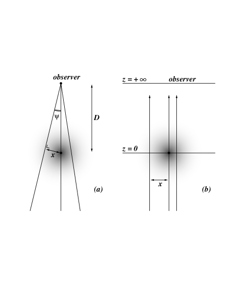
Figure 1: The two coordinate systems as described in section 2. When the distance $D$ between the observer and the galaxy’s centre goes to infinity, figure (a) transforms into figure (b).

3 The model

3.1 The stellar component

Since dusty projections already require a double integration along the line-of-sight, one is inclined to use a dynamical model that is as simple as possible to avoid cumbersome numerical work. Therefore the Plummer model (Dejonghe 1987), representing a spherical cluster without central singularity, seems an obvious candidate. Although the photometry of this model does not fit real elliptical galaxies, it has the huge advantage that the entire kinematic structure is sufficiently rich to include radial and tangential models, and that it can be described analytically. We can safely assume that our results will be generic for the class of elliptical galaxies.

We fix the units by choosing a value for the total stellar mass $M$, the gravitational constant $G$ and a scale length $r_{*}$. Working in dimensionless units we choose $M=G=r_{*}=1$. For the potential we choose the natural unit $\psi_{*}=G\,M/r_{*}$ and we set $\psi(0)=1$. In these units the central escape velocity equals $\sqrt{2}$, and the Plummer model is defined by

$$\psi(r)=\frac{1}{\sqrt{1+r^{2}}}$$ (7a)

$$\rho(r)=\frac{3}{4\pi}\,\left(1+r^{2}\right)^{-\frac{5}{2}}.$$ (7b)

Dejonghe (1986) describes a technique to construct 2-integral distribution functions $F(E,L)$ that self-consistently generate a given potential-density pair, based on the construction of an augmented mass density $\tilde{\rho}(\psi,r)$, i.e. the density expressed as a function of $r$ and $\psi$. For the potential-density pair (7a,b) the following one-parameter family is convenient

$$\tilde{\rho}(\psi,r)=\frac{3}{4\pi}\,\psi^{5-q}\,\left(1+r^{2}\right)^{-\frac{q}{2}}.$$ (8)

This results in a family of completely analytical anisotropic Plummer models, fully described by Dejonghe (1987). The distribution function $F_{q}(E,L)$ and its moments can be expressed analytically. For example, the radial and tangential velocity dispersions read

$$\sigma_{r}^{2}(r)=\frac{1}{6-q}\frac{1}{\sqrt{1+r^{2}}}$$ (9a)

$$\sigma_{\phi}^{2}(r)=\sigma_{\theta}^{2}(r)=\frac{1}{6-q}\frac{1}{\sqrt{1+r^{2}}}\left(1-\frac{q}{2}\,\frac{r^{2}}{1+r^{2}}\right),$$ (9b)

and Binney’s anisotropy parameter equals

$$\beta(r)=1-\frac{\sigma_{\phi}^{2}}{\sigma_{r}^{2}}=\frac{q}{2}\,\frac{r^{2}}{1+r^{2}}.$$ (10)

This expression provides the physical meaning of the parameter $q$. It has the same sign as $\beta(r)$, and its range is restricted to $-\infty<q\leqslant 2$ (since $-\infty<\beta(r)\leqslant 1$). Tangential clusters have $q<0$, radial clusters have $0<q\leqslant 2$ and for $q=0$ the model is isotropic. For small radii all models are fairly isotropic, while the true nature of the orbital structure becomes clearly visible in the kinematics at radii $r\gg 1$. More specifically, we consider a tangential model ($q=-6$), a radial one ($q=1$) and the isotropic case ($q=0$).

3.2 The dust component

A dust model is completely determined by its opacity function $\kappa(r)$. Besides the geometrical dependency, this function is also dependent upon the wavelength, which we do not mention explicitly. WTC92 considered an elliptical galaxy model with a diffusely distributed dust component. They used a King profile for both the stellar and the dust component. Analogous models were considered by Goudfrooij & de Jong (1995) and WS96. In the assumption that dust is only present in the inner part of ellipticals, WTC92 cut off the dust distribution at two thirds of the galaxy radius. Nevertheless dust may also be present in the outer regions, with temperatures of the order of 20 K (Jura 1982, Goudfrooij & de Jong 1995).

Our dust model is defined by the opacity function

$$\kappa(r)=\frac{1}{\sqrt{\pi}}\,\tau\,\frac{\Gamma\left(\frac{\alpha}{2}\right)}{\Gamma\left(\frac{\alpha-1}{2}\right)}\,\frac{1}{r_{0}}\,\left(1+\frac{r^{2}}{r_{0}^{2}}\right)^{-\frac{\alpha}{2}},$$ (11)

with $r_{0}$ a scale factor and $\alpha$ the so-called dust exponent. The normalization is such that $\tau$ equals the total optical depth (in the $V$-band), defined as

$$\tau=2\int_{0}^{+\infty}\kappa(r)\,{\rm d}r.$$ (12)

We can calculate the weight function ${\cal K}(x,r)$ by substituting (11) in (6b),

$${\cal K}(x,r)=\exp\left(-\frac{\tau(x)}{2}\right)\,\cosh\left[\frac{\tau(x)}{2}\,{\bf U}_{\alpha-3}\!\left(\sqrt{\frac{r^{2}-x^{2}}{r^{2}+r_{0}^{2}}}\right)\right],$$ (13)

where $\tau(x)$ is the optical depth along a line-of-sight $x$

$$\tau(x)=2\,\int_{x}^{+\infty}\frac{\kappa(r)\,r\,{\rm d}r}{\sqrt{r^{2}-x^{2}}}=\tau\,\left(1+\frac{x^{2}}{r_{0}^{2}}\right)^{-\frac{\alpha-1}{2}},$$ (14)

and the function ${\bf U}_{\alpha}(z)$ is defined in appendix A.

3.3 Parameter space

3.3.1 The optical depth

The optical depth is an indicator of the amount of dust in the galaxy, and is therefore the primary parameter in the models. WS96 estimated the optical depths of a sample of ellipticals by fitting radial colour gradients and found a median value of $\tau\la 2$. We explore optical depths between $\tau=0.1$ and $\tau=200$.

3.3.2 The dust geometry

The parameters $r_{0}$ and $\alpha$ determine the shape of the dust distribution. The exponent $\alpha$ is restricted to $\alpha>1$. Smaller values of $\alpha$ or larger values of $r_{0}$ correspond to extended distributions; for larger values of $\alpha$ or smaller values of $r_{0}$ the dust is more concentrated in the central regions. Since the two geometry parameters $r_{0}$ and $\alpha$ have roughly the same effect, we concentrate upon the case $r_{0}=1$ and we take $\alpha$ as the parameter determining the geometry.

For high values of $\alpha$ the distribution is very concentrated in the central regions of the galaxy. HST imagery has revealed compact dust features in the majority of the nearby ellipticals (van Dokkum & Franx 1995), and these could be an indication of an underlying concentrated diffuse dust distribution. However, Silva & Wise (1996) showed that such smooth dust concentrations should induce easily detectable colour gradients in the core, even for small optical depths. But high resolution HST imaging of two samples of nearby ellipticals revealed that elliptical galaxy cores have usually small colour gradients (Crane et al. 1993, Carollo et al. 1997), and thus no direct indication of concentrated diffuse dust is found. Therefore high values of $\alpha$ seem to be less probable and we will only treat them for the sake of completeness.

On the other hand, for small values of the dust component the distribution will be extended. If $\alpha$ approaches 1 the distribution is very extended, and little dust is located in the central regions of the galaxy. In the limit the dust is infinitely thin distributed over all space, the contribution of the dust in the galaxy is zero and the dust effectively forms an obscuring layer between the galaxy and the observer. This geometry is known as the overlying screen model (Holmberg 1975, Disney et al. 1989) and is the analogue for extinction of galaxian stars. By taking the limit $\alpha\rightarrow 1$ in (14) we obtain

$$\tau(x)=\tau$$ (15)

and substitution in (13) yields

$${\cal K}(x,r)=\exp\left(-\frac{\tau}{2}\right).$$ (16)

Notice that the same result can be found by taking the limit $r_{0}\rightarrow+\infty$.

As demonstrated in section 2, the computational prize of dust absorption on the projection of kinematic quantities is a double integration along the line-of-sight instead of a single one. This can be avoided if the weight function ${\cal K}(x,r)$ can be calculated analytically for all $x$ and $r$, i.e. if the functions ${\bf U}_{\alpha-3}(z)$ can be evaluated explicitly. For obvious computational reasons, we concentrate on the cases where $\alpha$ is an integer number. But to study the effects in the neighborhood of the singular value $\alpha=1$, we also consider a range of non-integer values for $\alpha$ between 1 and 2.

4 The projected kinematics

For the dust-free model all the moments of a line profile can be calculated analytically (see appendix B). For the lower order moments we find

$$\rho_{p}(x)=\frac{1}{\pi}\frac{1}{\left(1+x^{2}\right)^{2}},$$ (17)

and

$$\sigma_{p}^{2}(x)=\frac{9\pi}{32}\,\frac{1}{6-q}\,\frac{1}{\sqrt{1+x^{2}}}\left(1-\frac{5\,q}{12}\,\frac{x^{2}}{1+x^{2}}\right).$$ (18)

For dusty models this projection has to be carried out numerically. We calculated the projected mass density, the projected velocity dispersion and a set of line profiles for our dusty galaxy models. In this section we compare the normal and the dusty projections of the kinematic quantities, and we investigate both the dependence upon the optical depth $\tau$ and upon the dust geometry.

4.1 Dependence upon optical depth

In this section we keep the dust geometry fixed and vary the optical depth $\tau$. We adopt a modified Hubble profile ($\alpha=3$), which is slightly more extended than the stellar light.

4.1.1 The projected density

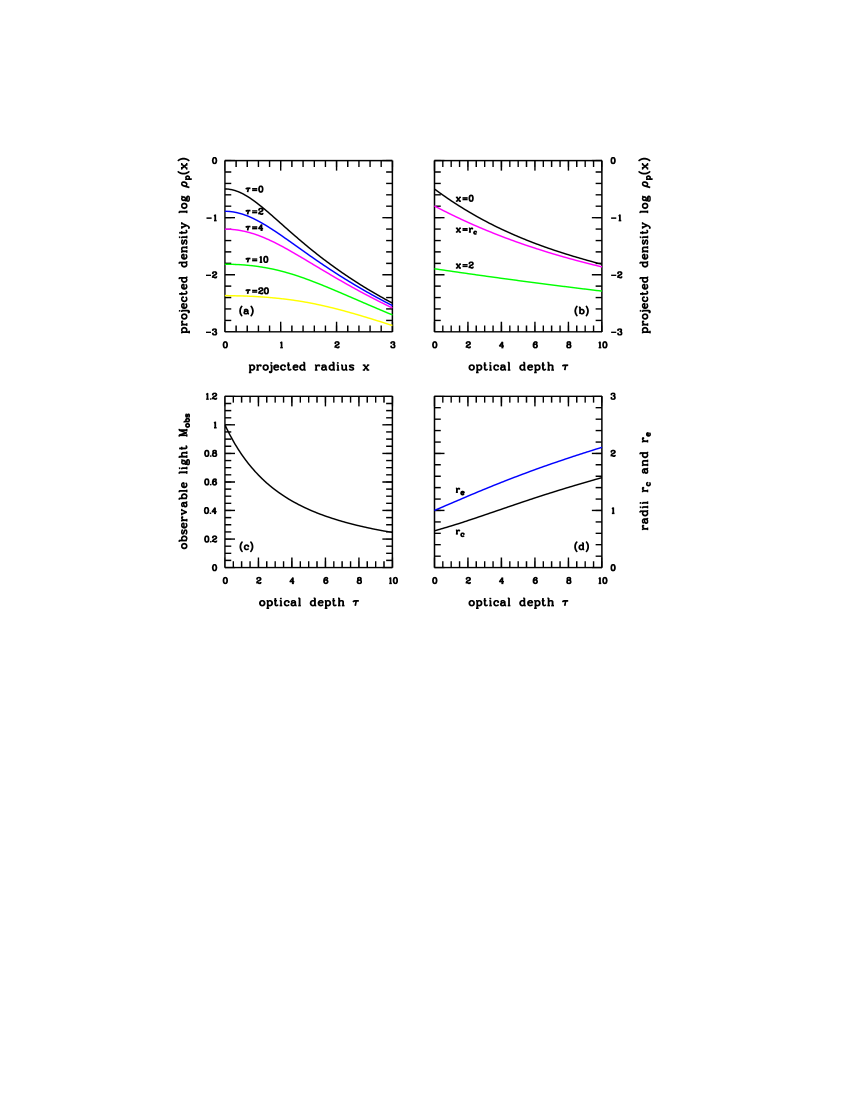
Figure 2: The dependence of the projected density $\rho_{p}(x)$ upon the optical depth $\tau$. The dust model is the $\alpha=3$ model. In panel (a) the projected density is plotted as a function of the projected radius $x$ for various values of $\tau$, which are indicated. In figure (b) we show the projected density explicitly as a function of the optical depth $\tau$, for three lines-of-sight $x$. The curve for $x=0$ can be calculated explicitly, as done in appendix B. The lower two panels show (c) the total integrated light $M_{\rm obs}$, and (d) the core radius $r_{c}$ and the effective radius $r_{e}$ as a function of $\tau$.

The primary effect of dust absorption on the projected density profile (figure 2a,b) is obvious : an overall reduction. Even for modest amounts of dust this effect is clearly observable. The projected density in the central regions is already reduced to half of its original value for an optical depth $\tau=1.5$. At the core radius $r_{c}=0.64$ this occurs for $\tau=3$. The global effect of the extinction is shown in figure 2c, which displays the observed integrated light $M_{\rm obs}$, i.e. the fraction of the total light output that can be detected by the observer. It is obtained by integrating the projected density profile $\rho_{p}(x)$ over the entire plane of the sky,

$$M_{\rm obs}=2\pi\,\int_{0}^{+\infty}\rho_{p}(x)\,x\,{\rm d}x.$$ (19)

The global extinction effect is strong : for an optical depth $\tau=1$ already 20 per cent of the mass is hidden for the observer, and for $\tau=3.4$ this becomes 50 per cent.

Besides reducing the amount of starlight, the dust has also a qualitative effect on the projected density profile. Since the dust is primarily located in the central portions of the galaxy, the $\rho_{p}(x)$ profile will be flattened towards the centre. As shown by WTC92 and WS96 this causes the production of colour gradients. But it has also a non-negligible effect on all global photometric quantities, e.g. luminosities and core and global diameters. For example, the apparent core of the galaxy (quantified by the core radius $r_{c}$ or the effective radius $r_{e}$) will be larger due to the central flattening (figure 2d). This effect can be up to 25 per cent or more for our basic model with moderate optical depths $\tau\approx 2$. On the other hand the total diameter of the galaxy (usually expressed as the diameter of the 25 mag arcsec^-2 isophote) will appear smaller due to the global attenuation.

4.1.2 The projected dispersion

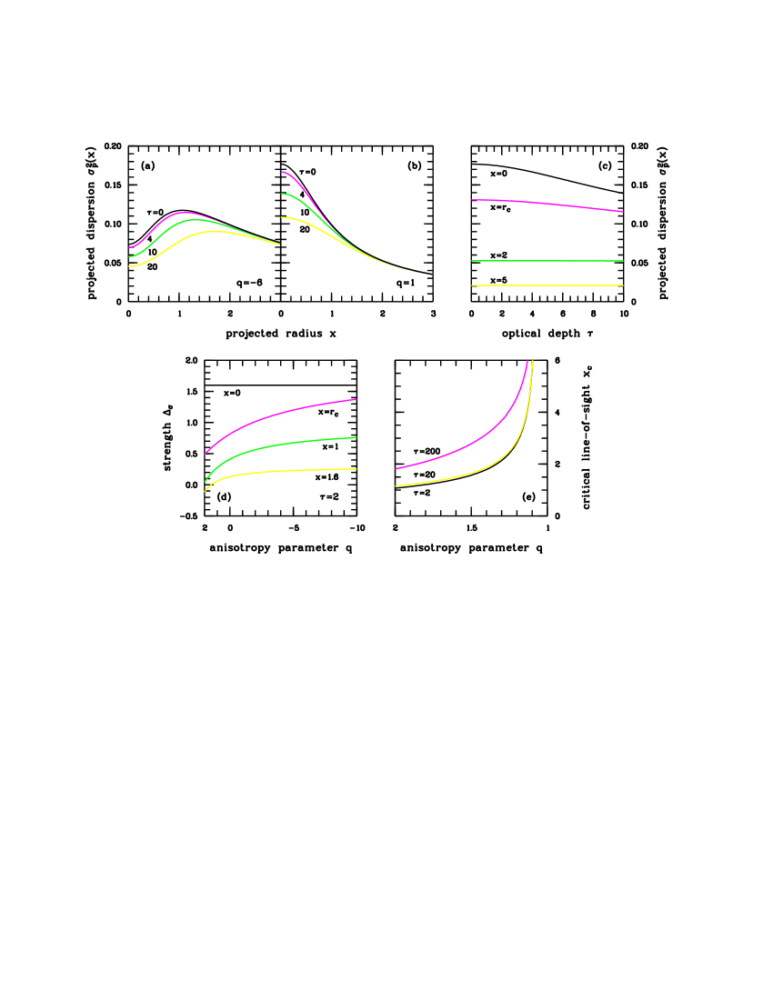
Figure 3: The dependence of the projected dispersion $\sigma_{p}^{2}(x)$ upon the optical depth $\tau$. The dust model is the $\alpha=3$ model. In the upper two panels the projected dispersion is plotted as a function of the projected radius $x$ for various values of $\tau$, which are indicated. It is shown (a) for a tangential model with $q=-6$ and (b) a radial model with $q=1$. In panel (c) we show the projected dispersion explicitly as a function of the optical depth $\tau$, for four lines-of-sight $x$. It is plotted for the radial model $q=1$. The curve for $x=0$ can be calculated explicitly, as done in appendix B. In figure (d) we plot the strength $\Delta_{\sigma}(x)$ of the effect on the dispersion profile as a function of the anisotropy parameter $q$ for three different lines-of-sight, which are indicated. The optical depth is $\tau=2$. The last plot (e) displays the critical line-of-sight $x_{c}$ for which $\Delta_{\sigma}(x_{c})=0$ as a function of the anisotropy parameter $q$, for different values of $\tau$. Above these curves the parameter has negative values, below are positive values.

The effect of dust on the projected dispersion profile $\sigma_{p}^{2}(x)$ has a totally different nature than the effect on the projected density profile $\rho_{p}(x)$, since it is a normalized projection. For a particular line-of-sight $x$ the weight function ${\cal K}(x,r)$ is responsible for the fact that not all parts of that line-of-sight contribute in the same proportion to the dusty projection, as is the case in the optically thin regime. From equation (13) and appendix A we can see that the weight function is a monotonically rising function of $r$ for all lines-of-sight $x$, essentially because along a line-of-sight the near side dominates the light. Dust makes the contribution of the outer parts (in particular the near side) thus more important, relative to the inner parts.

In figure 3a,b we plot the projected velocity dispersion profile $\sigma_{p}^{2}(x)$ for various optical depths. The explicit dependence of $\sigma_{p}^{2}(x)$ on $\tau$ for a fixed line-of-sight $x$ is shown in figure 3c. From these figures it is clear that quantitatively, the effects of dust absorption on the projected velocity dispersion are rather limited. Particularly for modest optical depths, $\tau\la 2$, there is no major difference between normal and dusty projection of the dispersion. In figure 3d we plot the strength (in percentage)

$$\Delta_{\sigma}(x)\equiv 100\times\frac{\left.\sigma_{p}^{2}(x)\right|_{\tau=0}-\left.\sigma_{p}^{2}(x)\right|_{\tau}}{\left.\sigma_{p}^{2}(x)\right|_{\tau=0}}$$ (20)

of the effect as a function of the anisotropy parameter $q$. It is shown for a set of lines-of-sight, with $\tau=2$. The effect is only 1.6 per cent for the central line-of-sight, independent of the anisotropy of the model. At larger radii this anisotropy does become important, tangentially anisotropic systems are more sensitive to dust in their $\sigma_{p}^{2}(x)$ profile than their radial counterparts. At $x=r_{c}$ this drops to 1.2 per cent for the tangential and to 0.7 per cent for the radial model.

Qualitatively, the general effect of dust is to lower the projected dispersion profile, and mostly $\Delta_{\sigma}$ will be a positive quantity. Only for the outer lines-of-sight of very radially anisotropic models the effect has the opposite sign, i.e. the projected dispersion is higher for the optically thick than for the optically thin case. In figure 3e we plot the critical line-of-sight $x_{c}$ where $\Delta_{\sigma}(x_{c})=0$ as a function of $q$, for various values of $\tau$. Notice that its dependence upon the optical depth is very weak.

4.1.3 The line profiles

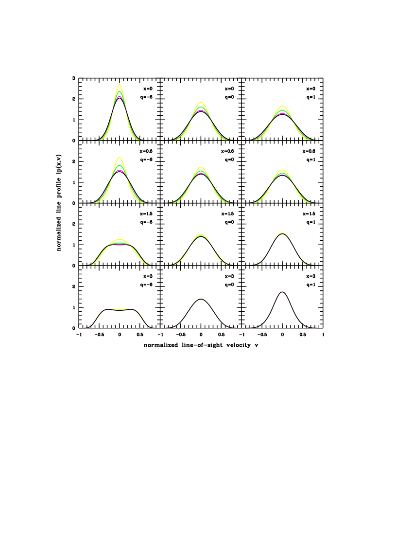
Figure 4: A set of normalized line profiles for our standard dust model ($r_{0}=1$ and $\alpha=3$) for varying optical depth. The left, middle and right column correspond to respectively the radial, isotropic and tangential models. The line-of-sight $x$ is indicated. Line profiles are shown for $\tau=0$, $\tau=4$, $\tau=10$ and $\tau=20$, going from black to light-coloured grey. Both the line-of-sight velocities and the area under the curves are normalized, as described in the text.

In figure 4 a number of normalized line-profiles ${\rm lp}(x,v)$ are plotted, for a set of lines-of-sight varying from the centre to the outer parts of the galaxy. The line-of-sight velocities $v$ are normalized with respect to the largest possible velocity one can observe at the particular line-of-sight $x$, being the escape velocity $\sqrt{2\,\psi(x)}$, where $\psi(r)$ is the Plummer potential (7a). The total area under the line profile, which equals the zeroth moment $\rho_{p}(x)$, is scaled to one.

The effect of dust absorption on a normalized line-profile ${\rm lp}(x,v)$ is at first order determined by the effect on its second moment, i.e. the projected dispersion $\sigma^{2}_{p}(x)$ at that projected radius. We can therefore copy most of our findings from the previous section. Only for higher optical depths and the inner lines-of-sight the influence of dust absorption is significant. In most cases dust absorption will turn the line profiles more peaked, and again tangential models are more sensitive to this than radial ones.

A particular consequence is that the typical bimodal structure of the outer line profiles of tangential models can disappear (see the $x=1.5$ line profile in figure 4). Physically this can be understood in the following way. In a tangentially anisotropic model, most of the stars move on rather circular orbits, particularly in the outer parts. Since the density of the Plummer model follows a strong $r^{-5}$ at large radii, the line profiles are primarily governed by the stars which move at orbits with radius $r\approx x$ (in both senses), causing the bimodal structure. When the system is heavily obscured, the nearest parts of the line-of-sight contribute relatively more than in the optically thin case. And these nearest parts contain stars moving on nearly circular orbits with larger radii, which have velocities that are gradually more perpendicular to the line-of-sight. Moreover these stars have smaller velocities anyway, since the circular velocity for the Plummer geometry declines as $r^{-1/2}$ at large radii. Smaller line-of-sight velocities thus become predominant, which causes the bimodal structure to disappear.

4.2 Dependence upon dust geometry

In this section we vary the dust exponent between $\alpha=1$ and $\alpha=10$, while the optical depth is held fixed. We choose large values for $\tau$ ($\tau=10$ and $\tau=20$) so that the geometry effect is clearly visible.

4.2.1 The projected density

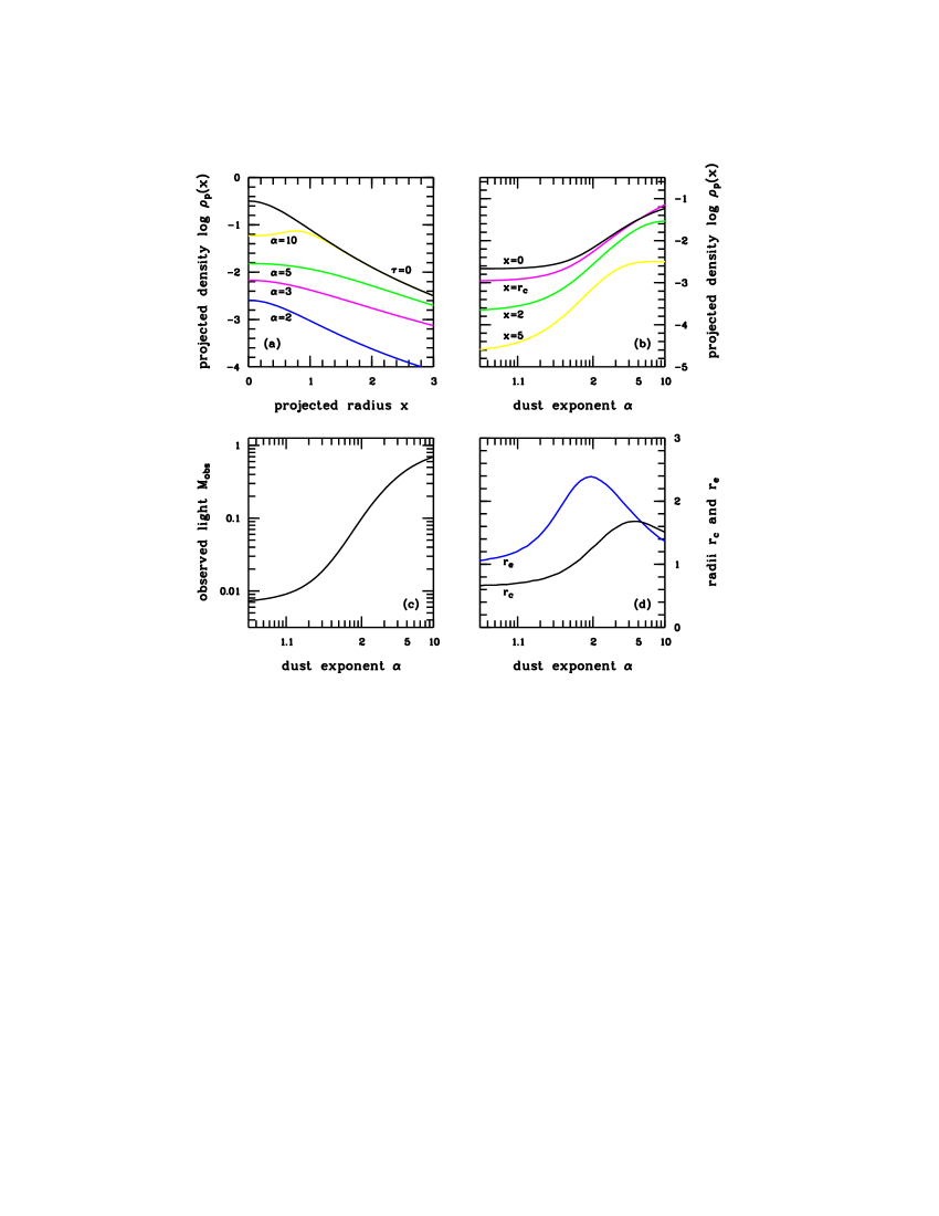
Figure 5: The dependence of the projected density $\rho_{p}(x)$ upon the dust exponent $\alpha$, with $\tau=10$. In panel (a) the projected density is plotted as a function of the projected radius $x$ for various values of $\alpha$, which are indicated. Figure (b) shows the projected density as a function of $\alpha$, for four lines-of-sight $x$. The lower two panels show (c) the total integrated light $M_{\rm obs}$, and (d) the core radius $r_{c}$ and the effective radius $r_{e}$ as a function of $\alpha$.

The dependence of $\rho_{p}(x)$ on the dust exponent $\alpha$ is shown in figure 5a and 5b, where we adopt the optical depth $\tau=10$. As is to be expected, the projected density $\rho_{p}(x)$ is sensitive to variations of the dust geometry parameters. In the outer regions (the bottom curves in figure 5b) this is primarily due to the optical depth profile (14) which depends critically on $\alpha$. Smaller values of $\alpha$ mean more dust and therefore more extinction. But also in the inner regions (black curve in figure 5b) the extinction effect is larger for extended than for concentrated distributions, even though equal amounts of dust are present. At each projected radius $x$ and for each optical depth $\tau$, the projected density $\rho_{p}(x)$ is a rising function of $\alpha$, with lowermost value

$$\lim_{\alpha\rightarrow 1}\rho_{p}(x)=\frac{1}{\pi}\,{\rm e}^{-\frac{\tau}{2}}\,\frac{1}{\left(1+x^{2}\right)^{2}}.$$ (21)

As a consequence, the total integrated light $M_{\rm obs}$ increases with $\alpha$ too (figure 5c), with $\exp\left(-\tfrac{\tau}{2}\right)$ for the overlying screen model being the minimum value. The more the dust is distributed homogeneously over the line-of-sight, the more efficient the extinction process.

Also the morphology of the $\rho_{p}(x)$ profile is sensitive for variations of the dust geometry (figure 5a). For small values of $\alpha$ the effect is small, and in the limit of the screen geometry the effect is nil : the projected density decreases with the same factor for all lines-of-sight. For larger values of $\alpha$, the profile becomes flatter in the centre. For very condensed dust distributions the extinction is confined to the central parts of the galaxy.

The dependence of the core radius $r_{c}$ and the effective radius $r_{e}$ on $\alpha$ is illustrated in figure 5d. The maximum effect on these core size parameters is found at intermediate values of $\alpha$. For very extended distributions on the one hand, the entire $\rho_{p}(x)$ profile is affected with the same factor, and as a consequence the core size parameters are not affected. For very concentrated distributions on the other hand only the inner part of the core is affected, so that the total light output of the core remains nearly the same.

4.2.2 The projected dispersion

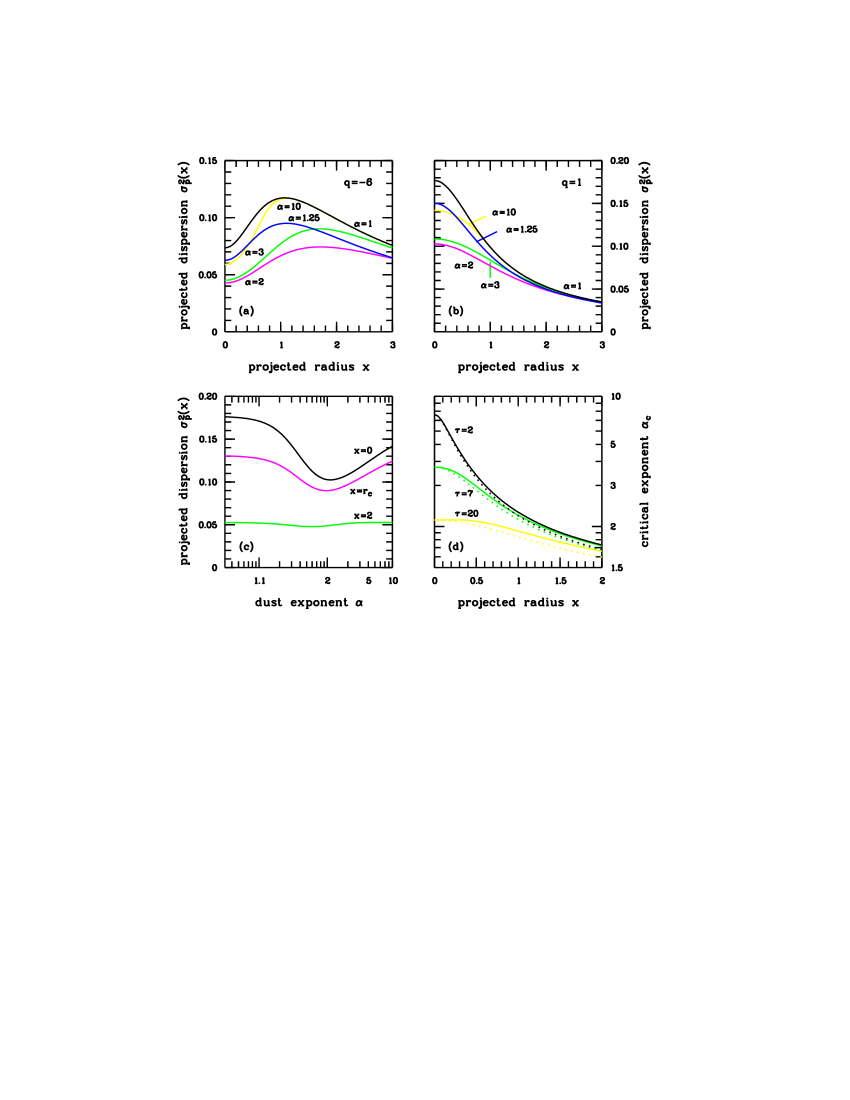
Figure 6: The dependence of the projected dispersion $\sigma_{p}^{2}(x)$ upon the dust exponent $\alpha$. The optical depth is fixed at the value $\tau=20$ for these plots. In the upper two panels $\sigma_{p}^{2}(x)$ is plotted as a function of the projected radius $x$ for various dust geometries, which are indicated. It is shown (a) for a tangential model with $q=-6$ and (b) a radial model with $q=1$. In panel (c) we show the projected dispersion explicitly as a function of the optical depth $\alpha$, for three lines-of-sight $x$. It is plotted for the radial model $q=1$. In plot (d) we plot the critical dust exponent $\alpha_{c}$ (see text) as a function of the projected radius $x$ for various optical depths and orbital models. The values of $\tau$ are indicated. The solid lines correspond to the radial $q=1$ model, the dotted lines to the tangential $q=-6$ models.

The primary effect of dust absorption on the projected dispersion $\sigma^{2}_{p}(x)$ at a certain line-of-sight $x$ is to attach a weight to every part of that line-of-sight. Or, since both halves of our Plummer galaxy are dynamically equivalent, to every part of the nearer half of the line-of-sight. Since the parameter $\alpha$ controls the relative distribution of the dust along the lines-of-sight, this parameter determines in the first place the relative weights of the different parts.

There are two extreme cases. For very concentrated models on the one hand, the entire first half of the line-of-sight is not affected. For very extended models on the other hand, the dust is effectively located between the observer and the galaxy, and all the parts of the line-of-sight $x$ experience the same influence, and thus have the same relative weight. We obtain that for both cases, each part of the nearer half of the line-of-sight contributes equally to the projected dispersion, as in the optically thin limit. The dusty projected dispersion profile $\sigma^{2}_{p}(x)$ therefore equals the optically thin profile (18), no matter how large the optical depth $\tau$.

For the dust models considered here, the relative weights do differ from each other, and there is an effect on the projected dispersion profile. In the figures 6a and 6b we plot the $\sigma_{p}^{2}(x)$ profile for various values of $\alpha$, for a fixed optical depth $\tau=20$. For every line-of-sight there is a critical exponent $\alpha_{c}$ that corresponds to the most efficient dust geometry. This is illustrated in figure 6c, where $\sigma_{p}^{2}(x)$ is plotted as a function of $\alpha$ for various lines-of-sight. Notice that the position of the critical dust exponent $\alpha_{c}$ not only depends on the line-of-sight $x$, but also on the optical depth $\tau$ and the anisotropy parameter $q$. This is shown in figure 6d, where $\alpha_{c}$ is plotted as a function of $x$ for different values of $\tau$ and $q$.

4.2.3 The line profiles

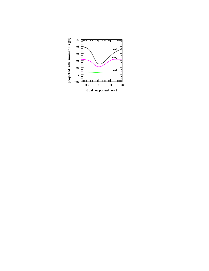
Figure 7: The projected fourth moment $\tau_{p}^{4}(x)$ as a function of the dust exponent $\alpha$ for a set of lines-of-sight $x$. The optical depth is $\tau=20$, the model is the radial $q=1$ model.

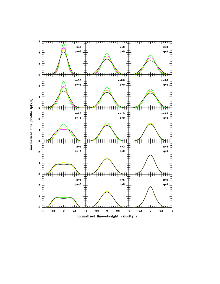
Figure 8: A set of normalized line profiles ${\rm lp}(x,v)$ for various values of the dust exponent $\alpha$ and a fixed optical depth $\tau=20$. The left, middle and right column correspond to respectively the radial, isotropic and tangential models. The line-of-sight $x$ is indicated. Line profiles are shown for the optically thin model and for $\alpha=5$, $\alpha=2$ and $\alpha=1.25$, going from black to light-coloured grey. Both the line-of-sight velocities and the area under the curves are normalized.

The reasoning from the previous section does not only apply to the projected dispersion profile, but to all higher order moments of a line profile (for a definition, see appendix B). For each line-of-sight $x$, such a higher order projected moment equals its optically thin value for very concentrated or very extended models, and there is an intermediate critical value $\alpha_{c}$ for which the effect is maximal. This is illustrated in figure 7, where we plot the projected fourth moment $\tau_{p}^{4}(x)\equiv\mu_{p}^{4}(x)/\rho_{p}(x)$ for various lines-of-sight, as a function of the dust exponent $\alpha$. The analogy with figure 6c is obvious. Notice that the critical dust exponent $\alpha_{c}$ differs from moment to moment. For example, for the line-of-sight through the centre we find $\alpha_{c}=2.115$ for the projected dispersion, and $\alpha_{c}=2.215$ for the fourth moment.

The same applies to the line profiles themselves (figure 8). For the two limit cases, there is no difference between optically thick and optically thin models, no matter how high the optical depth. And for each line-of-sight $x$, each optical depth $\tau$ and each orbital model $q$ there is a critical dust exponent $\alpha_{c}$, for which the effect of dust absorption on the line profiles is maximal. The extent to which $\alpha$ differs from this critical value determines the magnitude of the effect on the line profile.

5 Conclusions

Comparison of optical and IRAS data suggests that elliptical galaxies are likely to contain a diffuse dust component, which is smoothly distributed over the galaxy (Goudfrooij & de Jong 1995). Dust absorption affects the projection of all physical quantities along a line-of-sight. We constructed a four-parameter model to investigate the absorption effects on the projection of kinematic quantities. We compared the optically thick with the optically thin case, and investigated the effects of optical depth and dust geometry.

We established that the projected mass density $\rho_{p}(x)$ is substantially affected, even for modest optical depths ($\tau\la 2$). Dust has also a non-negligible effect on the morphology of the $\rho_{p}(x)$ profile and on all global photometric quantities. On the other hand, the effects of dust absorption on the projected velocity dispersion profile $\sigma^{2}_{p}(x)$ and on the line profiles are considerable only for higher optical depths ($\tau\ga 5$). Moreover, the dust geometry is important : both centrally concentrated and very extended dust distributions can remain invisible in the line profiles.

Our models have some important applications, which are being investigated :

• Due to the insensitivity of the $\sigma_{p}^{2}(x)$ profile, dynamical mass estimates will hardly be affected by modest amounts of dust, while the light profile is sensitive for absorption. This should be taken in consideration in the interpretation of mass-to-light ratios in regions where no dark matter is expected : large mass-to-light ratios can indicate dust absorption.

• All global photometric properties of elliptical galaxies such as luminosities and radii are affected by dust. As WS96 pointed out, this can lead to a systematic uncertainty in elliptical galaxy distance estimation techniques that utilize these global properties, e.g. the $L$-$\sigma$ relation (Faber & Jackson 1976) or the relations of the fundamental plane (Dressler et al. 1987, Djorgovski & Davis 1987). With our models, we can not only quantify the effect of dust on the global photometric properties, but also on the kinematics.

• While large optical depths don’t seem to be in accordance with global IRAS dust mass estimates, these models are nevertheless important on a local scale. Compact regions with high optical depths can be an explanation for the observed asymmetries and irregularities in kinematic data. In that case, one needs to combine (basically dust-free) near-infrared data with optical data. Such observations would help to constrain the diffuse dust masses in elliptical galaxies, a problem which cannot be satisfyingly solved with the existing methods.

Appendix A The function ${\bf U}_{\alpha}(z)$

Figure 9: The function ${\bf U}_{\alpha}(z)$ for different values of $\alpha$. The values of $\alpha$ are indicated.

For $\alpha>-2$ and for $0\leqslant z\leqslant 1$ the function ${\bf U}_{\alpha}(z)$ is defined as

$${\bf U}_{\alpha}(z) =\int_{0}^{z}\left(1-y^{2}\right)^{\frac{\alpha}{2}}\,{\rm d}y\left/\int_{0}^{1}\left(1-y^{2}\right)^{\frac{\alpha}{2}}\,{\rm d}y.\right.$$

$$=\frac{2}{\sqrt{\pi}}\,\frac{\Gamma\left(\frac{\alpha+3}{2}\right)}{\Gamma\left(\frac{\alpha+2}{2}\right)}\,\int_{0}^{z}\left(1-y^{2}\right)^{\frac{\alpha}{2}}\,{\rm d}y$$ (22)

For natural values of $\alpha$ it can be easily calculated with the recursion formula

$${\bf U}_{\alpha}(z)={\bf U}_{\alpha-2}(z)+\frac{1}{\sqrt{\pi}}\,\frac{\Gamma\left(\frac{\alpha+1}{2}\right)}{\Gamma\left(\frac{\alpha+2}{2}\right)}\,z\,\left(1-z^{2}\right)^{\frac{\alpha}{2}}$$ (23)

together with the seeds

$${\bf U}_{-1}(z)=\frac{2}{\pi}\,\arcsin(z)$$ (24)

$${\bf U}_{0}(z)=z.$$ (25)

The functions ${\bf U}_{\alpha}(z)$ can also be written in terms of the hypergeometric function, which is convenient for computational purposes if $\alpha$ is non-integer,

$${\bf U}_{\alpha}(z)=\frac{2}{\sqrt{\pi}}\,\frac{\Gamma\left(\frac{\alpha+3}{2}\right)}{\Gamma\left(\frac{\alpha+2}{2}\right)}\,z\,_{2}F_{1}\left(\tfrac{1}{2},-\tfrac{\alpha}{2};\tfrac{3}{2};z^{2}\right).$$ (26)

In the limit $\alpha\rightarrow-2$ one finds the degenerate function

$$\lim_{\alpha\rightarrow-2}{\bf U}_{\alpha}(z)=\left\{\begin{array}[]{l@{\qquad}l}0&\mbox{for $0\leqslant z<1$}\\ 1&\mbox{for $z=1$.}\end{array}\right.$$ (27)

Appendix B The moments of the central line profile

Table 1: Analytical expressions for the central projected density $\rho_{p}(0)$ and the central projected dispersion $\sigma_{p}^{2}(0)$ as a function of the optical depth $\tau$. In all cases $r_{0}=1$, the value of $\alpha$ is indicated. The expressions for $\alpha=3$ and $\alpha=2$ correspond to equations (36) and (37). For $\alpha=5$ the projected density can be calculated by direct integration, for higher order moments no explicit expression can be deduced.

$\alpha$	$\rho_{p}(0)$	$\sigma_{p}^{2}(0)$
1	$\displaystyle\frac{1}{\pi}\,{\rm e}^{-\frac{\tau}{2}}$	$\displaystyle\left(\frac{1}{6-q}\right)\,\frac{9\pi}{32}$
2	$\displaystyle 9\pi^{3}\,{\rm e}^{-\frac{\tau}{2}}\,\frac{\cosh\left(\frac{\tau}{2}\right)}{(\tau^{2}+\pi^{2})\,(\tau^{2}+9\pi^{2})}$	$\displaystyle\left(\frac{1}{6-q}\right)\,\pi\,\tanh\left(\tfrac{\tau}{2}\right)\,\frac{(\tau^{2}+\pi^{2})\,(\tau^{2}+9\pi^{2})}{\tau\,(\tau^{2}+4\pi^{2})\,(\tau^{2}+16\pi^{2})}$
3	$\displaystyle\frac{6}{\sqrt{\pi}}\,{\rm e}^{-\frac{\tau}{2}}\,\tau^{-\frac{3}{2}}\,I_{\frac{3}{2}}\!\left(\tfrac{\tau}{2}\right)$	$\displaystyle\left(\frac{1}{6-q}\right)\,\frac{3\sqrt{\pi}}{2}\,\frac{1}{\sqrt{\tau}}\,\frac{I_{2}\!\left(\frac{\tau}{2}\right)}{I_{\frac{3}{2}}\!\left(\frac{\tau}{2}\right)}$
5	$\displaystyle\frac{1}{\pi}\,\frac{1-{\rm e}^{-\tau}}{\tau}$

The general moments $\mu_{2n,2m,2l}(r)$ of a distribution function $F(r,{\mn@boldsymbol{v}})$ are defined as

$$\mu_{2n,2m,2l}(r)=\int\!\!\int\!\!\int F(r,{\mn@boldsymbol{v}})\,v_{r}^{2n}v_{\theta}^{2m}v_{\phi}^{2l}\,{\rm d}{\mn@boldsymbol{v}},$$ (28)

where the integration ranges over all possible velocities. The moments $\mu_{2n}(r,x)$ of the projected velocity distribution along a line-of-sight $x$ at a particular point $(x,r)$ in space are

$$\mu_{2n}(x,r)=\sum_{i=0}^{n}\binom{n}{i}\,\frac{\left(r^{2}-x^{2}\right)^{n-i}\,x^{2i}}{r^{2n}}\,\mu_{2(n-i),2i,0}(r).$$ (29)

To obtain the $2n$’th moment of the line profile (or the projected $2n$’th moment) this has to be projected along the line-of-sight $x$, according to the recipe (6a,b),

$$\mu_{p}^{2n}(x)\equiv 2\,\int_{x}^{+\infty}{\cal K}(x,r)\,\frac{\mu_{2n}(x,r)\,r\,{\rm d}r}{\sqrt{r^{2}-x^{2}}}.$$ (30)

For the Plummer model, these projected moments can be evaluated analytically in the optically thin limit (Dejonghe 1987),

$$\mu_{p}^{2n}(x)=\frac{3\cdot 2^{n-2}}{\pi}\,\frac{\Gamma\left(6-q\right)\,\Gamma\left(n+\frac{1}{2}\right)\,\Gamma\left(\frac{n+4}{2}\right)}{\Gamma\left(n+6-q\right)\,\Gamma\left(\frac{n+5}{2}\right)}\left(1+x^{2}\right)^{-\frac{n+4}{2}}\\ \times\!\,_{3}F_{2}\left(-n,\frac{q}{2},\frac{n+4}{2};1,\frac{n+5}{2},\frac{x^{2}}{1+x^{2}}\right).$$ (31)

yielding equation (17) and (18) for the cases $n=0$ and $n=1$.

For dusty galaxy models, equation (30) cannot be calculated analytically for general lines-of-sight. Only for the central line-of-sight $x=0$ this is possible in a few cases, since the formulae become considerably easier. The sum (29) reduces to a single term,

$$\mu_{2n}(0,r) =\mu_{2n,0,0}(r)$$ (32)

$$=\frac{3\cdot 2^{n-2}}{\pi\sqrt{\pi}}\,\frac{\Gamma\left(n+\frac{1}{2}\right)\,\Gamma\left(6-q\right)}{\Gamma\left(6-q+n\right)}\,\left(1+r^{2}\right)^{-\frac{n+5}{2}},$$ (33)

yielding equation (7b) and (9a) for $n=0$ and $n=1$ respectively. If we substitute the weight function (13) of the King dust model, we obtain

$$\mu_{p}^{2n}(0)=c\,{\rm e}^{-\frac{\tau}{2}}\,\int_{0}^{1}\cosh\left(\tfrac{\tau}{2}\,{\bf U}_{\alpha-3}(z)\right)\left(1-z^{2}\right)^{\frac{n+2}{2}}{\rm d}z$$ (34)

where we set

$$c=\frac{3\cdot 2^{n-1}}{\pi\sqrt{\pi}}\,\frac{\Gamma\left(6-q\right)\,\Gamma\left(n+\frac{1}{2}\right)}{\Gamma\left(n+6-q\right)}.$$ (35)

Since ${\bf U}_{\alpha-3}(z)$ can generally only be expressed as a hypergeometric function, we cannot evaluate this integral explicitly, except for some special values of the dust exponent $\alpha$ for which ${\bf U}_{\alpha-3}(z)$ has a very simple form. For $\alpha=3$ the integral in (34) leads to a family of modified Bessel functions of the first kind (Gradshteyn & Ryzhik 1965, eq. 8.431),

$$\mu_{p}^{2n}(0)=4\sqrt{\pi}\,c\,\Gamma\left(\tfrac{n+4}{2}\right)\,{\rm e}^{-\frac{\tau}{2}}\,\tau^{-\frac{n+3}{2}}\,I_{\frac{n+3}{2}}\left(\tfrac{\tau}{2}\right).$$ (36)

For $\alpha=2$ we find (Gradshteyn & Ryzhik 1965, eq. 3.981)

$$\mu_{p}^{2n}(0)=\left\{\begin{array}[]{l@{\qquad}l}\displaystyle\frac{\pi^{n+4}\,c\,\Gamma(n+4)\,{\rm e}^{-\frac{\tau}{2}}\,\cosh\left(\tfrac{\tau}{2}\right)}{\prod_{j=0}^{(n+2)/2}\Bigl{(}\tau^{2}+(2j+1)^{2}\pi^{2}\Bigr{)}}&\mbox{if $n$ even}\\ \\ \displaystyle\frac{\pi^{n+4}\,c\,\Gamma(n+4)\,{\rm e}^{-\frac{\tau}{2}}\,\sinh\left(\tfrac{\tau}{2}\right)}{\tau\,\prod_{j=1}^{(n+3)/2}\Bigl{(}\tau^{2}+(2j)^{2}\pi^{2}\Bigr{)}}&\mbox{if $n$ odd}.\end{array}\right.$$ (37)

From these expressions one can find the expressions for the projected density $\rho_{p}(0)$ and the projected dispersion $\sigma_{p}^{2}(0)$, as tabulated in table 1.

References

- [1] Bally J., Thronson H. A., 1989, AJ, 97, 69
- [2] Bertola F., Galletta G., 1978, ApJ, 226, L115 333, 673
- [3] Carollo C. M., Franx M., Illingworth G. D., Forbes D. A., 1997, ApJ, 481, 710
- [4] Crane P., Stiavelli M., King I. R., Deharveng J. M., Albrecht R., Barbieri C., Blades J. C., Boksenberg A., Disney M. J., Jakobsen P., Kamperman T. M., Machetto F., Mackay C. D., Paresce F., Weigelt G., Baxter D., Greenfield P., Jedrzejewski R., Nota A., Sparks W. B., 1993, AJ, 106, 1371
- [5] Dejonghe H., 1986, Phys. Rep., 133, 225
- [6] Dejonghe H., 1987, MNRAS, 224, 13
- [7] Disney M. J., Davies J. I., Phillips S., 1989, MNRAS, 239, 939
- [8] Djorgovski S., Kormendy J., 1989, ARA&A, 27, 235
- [9] Dressler A., Lynden-Bell D., Burnstein D., Davies R., Faber S. M., Terlevich R. J., Wegner G., 1987, ApJ, 313, 42
- [10] Ebneter K., Balick B., 1985, AJ, 90, 183
- [11] Faber S. M., Jackson R. E., 1976, ApJ, 204, 668
- [12] Fich M., Hodge P., 1993, ApJ, 415, 75
- [13] Goudfrooij P., de Jong T., 1995, A&A, 298, 784
- [14] Gradshteyn I. S., Ryzhik I. M., 1965, Table of Integrals, Series and Products, Academic Press Inc., New York
- [15] Haas M., 1998, A&A, 337, L1
- [16] Hawarden T. G., Elson R. A. W., Longmore A. J., Tritton S. B., Corwin H. G. Jr., 1981, MNRAS, 196, 747
- [17] Holmberg E., 1975, Stars and Stellar Systems IX, University of Chicago, 123
- [18] Jura M., 1982, ApJ, 254, 70
- [19] Jura M., 1986, ApJ, 306, 483
- [20] Knapp G. R., Guhathakurta P., Kim D.-W., Jura M., 1989, ApJS, 70, 329
- [21] Knapp G. R., Gunn J. E., Wynn-Williams C. G., 1992, ApJ, 399, 76
- [22] Mathis J. S., 1970, ApJ, 159, 263
- [23] Roberts M. S., Hogg D. E., Bregman J. N., Forman W. R., Jones C., 1991, ApJS, 75, 751
- [24] Sadler E. M., Gerhard O. E., 1985, MNRAS, 214, 177
- [25] van Dokkum P. G., Franx M., 1995, AJ, 110, 2027
- [26] Wiklind T., Henkel C., 1995, A&A, 297, L71
- [27] Wise M. S., Silva D. R., 1996, ApJ, 461, 155 [WS96]
- [28] Witt A. N., Thronson H. A. Jr., Capuano J. M. Jr., 1992, ApJ, 393, 611 [WTC92]