Extended High-Ionization Nuclear Emission-Line Region
in the Seyfert Galaxy NGC 4051

Abstract

We present an optical spectroscopic analysis of the well-known Seyfert galaxy NGC 4051. The high-ionization nuclear emission-line region (HINER) traced by [Fe X] $\lambda$6374 is found to be spatially extended to a radius of 3″ ($\approx$ 150 pc) west and southwest from the nucleus; NGC 4051 is the third example which has an extended HINER.

The nuclear spectrum shows that the flux of [Fe X] $\lambda$6374 is stronger than that of [Fe VII] $\lambda$6087 in our observation. This property cannot be interpreted in terms of a simple one-zone photoionization model.

In order to understand what happens in the nuclear region in NGC 4051, we investigate the physical condition of the nuclear emission-line region in detail using new photoionization models in which the following three emission-line components are taken into account; (1) optically thick, ionization-bounded clouds; (2) optically thin, matter-bounded clouds; and (3) a contamination component which emits H$\alpha$ and H$\beta$ lines. Here the observed extended HINER is considered to be associated with the low-density, matter-bounded clouds. Candidates of the contamination component are either the broad-line region (BLR) or nuclear star forming regions or both. The complexity of the excitation condition found in NGC 4051 can be consistently understood if we take account of these contamination components.

1. INTRODUCTION

It is known that Seyfert galaxies often show very high-ionization emission lines such as [Fe VII] $\lambda 6087$, [Fe X] $\lambda 6374$, [Fe XI] $\lambda 7892$ and [Fe XIV] $\lambda 5303$ (Oke & Sargent 1968; Grandi 1978; Penston et al. 1984; De Robertis & Osterbrock 1986). Because the ionization potentials of these lines are higher than 100 eV, much attention has been paid to the high-ionization nuclear emission-line region [HINER; Murayama, Taniguchi, & Iwasawa 1998 (hereafter MTI98); see also Binette 1985]. The possible mechanisms of radiating such high-ionization emission lines are the following three processes: (1) collisional ionization in the gas with temperatures of T_e $\sim$ 10⁶ K (Oke & Sargent 1968; Nussbaumer & Osterbrock 1970); (2) photoionization by the central nonthermal continuum emission [Osterbrock 1969; Nussbaumer & Osterbrock 1970; Grandi 1978; Korista & Ferland 1989; Ferguson, Korista, & Ferland 1997b; Murayama & Taniguchi 1998a, 1998b (hereafter MT98a and MT98b, respectively)]; and (3) a combination of shocks and photoionization (Viegas-Aldrovandi & Contini 1989).

Recently, in context of the locally-optimally emitting cloud models (LOC models; Ferguson et al. 1997a), Ferguson, Korista, & Ferland (1997b) showed that the high-ionization emission lines can be radiated in conditions of widely range of gas densities. More recently MT98a have found that type 1 Seyfert nuclei (S1s) have excess [Fe VII] $\lambda$6087 emission with respect to type 2s (S2s). Given the current unified model of AGN (Antonucci & Miller 1985; see for a review Antonucci 1993), the finding of MT98a implies that the HINER traced by the [Fe VII] $\lambda$6087 emission resides in the inner wall of such dusty tori. Since the covering factor of the torus is usually large (e.g., $\sim 0.9$), and the electron density in the tori (e.g., $\sim 10^{7\mbox{--}8}$ cm^-3) is considered to be significantly higher than that (e.g., $\sim 10^{3\mbox{--}4}$ cm^-3) of the narrow-line region (NLR), the contribution from the torus dominates the emission of the higher-ionization lines (Pier & Voit 1995). Taking this HINER component into account, MT98b have constructed new dual-component (i.e., a typical NLR with a HINER torus) photoionization models and explained the observations consistently.

On the other hand, it is also known that some Seyfert nuclei have an extended HINER whose size amounts up to $\sim$ 1 kpc (Golev et al. 1995; MTI98). The presence of such extended HINERs can be explained as the result of very low-density conditions in the interstellar medium ($n_{\rm H}\sim 1$ cm^-3) makes it possible to achieve higher ionization conditions (Korista & Ferland 1989). Thus MT98a suggested a three-component model for the spatial distribution of HINER in terms of photoionization. That is: (1) the inner wall of the dusty torus with electron densities of $n_{\rm e}\sim 10^{6\mbox{--}7}$ cm^-3; the torus HINER [Pier & Voit 1995; Murayama & Taniguchi 1998b], (2) the innermost part of the NLRs; the NLR HINER ($n_{\rm e}\sim 10^{3\mbox{--}4}$ cm^-3) at a distance from $\sim$10 to $\sim$100 pc, and (3) the extended ionized region ($n_{\rm e}\sim 10^{0\mbox{--}1}$ cm^-3) at a distance $\sim$1 kpc; the extended HINER (Korista & Ferland 1989; MTI98). Perhaps the relative contribution to the HINER emission from the above three components may be different from galaxy to galaxy. In particular, extended HINERs have been found only in NGC 3516 (Golev et al. 1995) and Tololo 0109–383 (MTI 98) and thus it is important to investigate how common the extended HINER in Seyfert galaxies.

In this paper, we report on the discovery of an extended HINER in the nearby Seyfert galaxy NGC 4051. This observation was made during the course of our long-slit optical spectroscopy program for a sample of nearby Seyfert galaxies at the Okayama Astrophysical Observatory. Throughout this paper, we use a distance toward NGC 4051 of 9.7 Mpc, which is estimated using a value of H₀ = 75 km s^-1 Mpc^-1 and its recession velocity of 726 km s^-1 (Ulvestad & Wilson 1984). Therefore, 1″ corresponds to 47 pc at this distance.

2. OBSERVATIONS

The spectroscopic observations were made at Okayama Astrophysical Observatory, National Astronomical Observatory of Japan on 1992 June 5. The New Cassegrain Spectrograph was attached to the Cassegrain focus of the 188 cm reflector. A 512 $\times$ 512 CCD with pixel size of 24 $\times$ 24 $\mu$m was used, giving a spatial resolution of 1$\farcs$46 pixel^-1 by 1 $\times$ 2 binning. A 1$\farcs$8 slit with a length of 300″ was used with a grating of 150 groove mm^-1 blazed at 5000 Å. The position angle was set to 90°. The wavelength coverage was set to 4500 – 7000 Å. We took three spectra; (1) the central region, (2) 2″ north of the central region, and (3) 2″ south of the central region. Each exposure time was 1200 seconds, respectively. The slit positions for NGC 4051 are displayed in Figure 1. The data was reduced with the use of IRAF. The reduction was made with a standard procedure; bias subtraction and flat fielding were made with the data of the dome flats. The flux scale was calibrated by using a standard star (BD+33^∘ 2642). The nuclear spectrum was extracted with 2$\farcs$92 aperture. The seeing size derived from the spatial profile of the standard star was about 2$\farcs$3 (FWHM) during the observations.

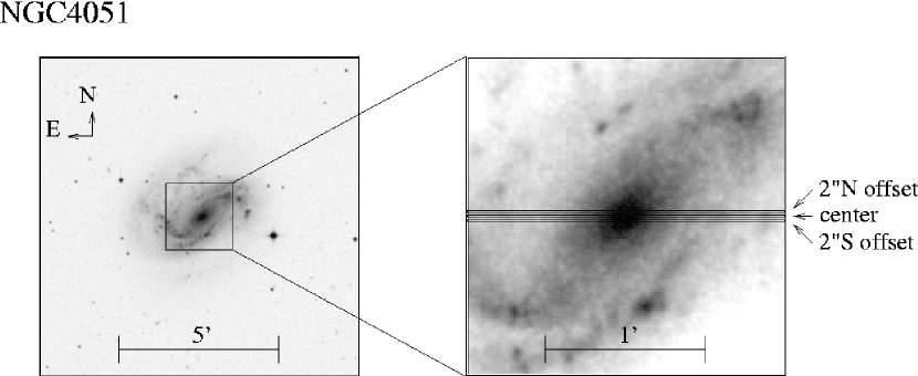
Figure 1.— Slit positions we set for NGC 4051. Images are taken from digitized sky survey.

3. OBSERVATIONAL RESULTS

3.1. Emission-Line Properties of the Nuclear Spectrum

The spectrum of the nuclear region (the central 2$\farcs$9 $\times$ 1$\farcs$8 region) is shown in Figure 2. In order to estimate emission-line fluxes, we made multicomponent Gaussian fitting for the spectrum using the SNG (the SpectroNebularGraph; Kosugi et al. 1995) package. The identified emission lines of the nuclear region are summarized in Table 1. The [Fe X] $\lambda$6374 emission line is blended with [O I] $\lambda$6364. Assuming the theoretical ratio of [O I] $\lambda$6300/[O I] $\lambda$6364 = 3 (Osterbrock 1989), we measured the [Fe X] $\lambda$6374 flux. The reddening was estimated by using the Balmer decrement (i.e., the ratio of narrow components of H$\alpha$ and H$\beta$). If the case B would be assumed, an intrinsic value of H$\alpha$/H$\beta$ ratio was 2.87 for $T$ = 10⁴ K (Osterbrock 1989). However, Veilleux & Osterbrock (1987) mentioned that the harder photoionizing spectrum of AGNs results in a large transition zone or partly ionized region in which collisional excitation becomes important (Ferland & Netzer 1983; Halpern and Steiner 1983). The main effect of the collisional excitation is to enhance H$\alpha$. Therefore we adopt H$\alpha$/H$\beta=$ 3.1 for the intrinsic ratio, and accordingly we obtain $A_{V}$ = 1.00 mag. This value is almost consistent with the previous estimation ($A_{V}$ = 1.11 mag: Erkens et al. 1997). In our observation, [Fe X] $\lambda$6374 (ionized potential 233.6 eV) is stronger than [Fe VII] $\lambda$6087 (99.1 eV). This observational result is inconsistent with the predictions of simple one-zone photoionization models (see section 4.).

Figure 2.— Nuclear spectrum of NGC 4051.

Table 1Emission-Line Data of the Nuclear Region in NGC4051

Identification	$\lambda_{{\rm obs}}$	FWHM	F/F(H$\beta$N)		I/I(H$\beta$N)
	(${\rm\AA}$)	(km s-1)	Line Ratios	1 $\sigma$	Line Ratios	1 $\sigma$
H$\beta$N	4874.6	934.2	1.000	—–	1.000	—–
[O III]	4970.7	431.3	0.457	$\pm$0.016	0.445	$\pm$0.015
[O III]	5018.7	427.1	1.348	$\pm$0.027	1.294	$\pm$0.026
[Fe XIV]	—–	—–	$<$0.071	—–	$<$0.063	—–
He I	5886.5	839.6	0.166	$\pm$0.014	0.130	$\pm$0.012
[Fe VII]	—–	—–	$<$0.080	—–	$<0$.060	—–
[O I]	6314.2	453.7	0.156	$\pm$0.012	0.113	$\pm$0.009
[O I]	6377.7	449.2	0.052	$\pm$0.012	0.037	$\pm$0.009
[Fe X]	6387.4	762.7	0.190	$\pm$0.014	0.136	$\pm$0.011
[N II]	6562.1	458.9	0.409	$\pm$0.017	0.286	$\pm$0.014
H$\alpha$N	6577.4	666.3	4.351	$\pm$0.073	3.030	$\pm$0.075
H$\alpha$B	6577.5	3439.7	2.285	$\pm$0.040	1.591	$\pm$0.035
[N II]	6597.4	456.4	1.208	$\pm$0.029	0.838	$\pm$0.028
[S II]	6733.5	—–	0.187	$\pm$0.012	0.127	$\pm$0.009
[S II]	6747.9	—–	0.201	$\pm$0.012	0.136	$\pm$0.009

In Table 2, we give a comparison between our observational data and the previous ones (Anderson 1970; Grandi 1978; Yee 1980; Penston et al. 1984; Veilleux 1988; Erkens, Appenzeller, & Wagner 1997). Although Erkens et al. (1997) gave [Fe VII] $\lambda$6087/[Fe X] $\lambda$6375 = 0.966 in their paper, they newly reduced their data and found the true observed line ratio is 0.500 (Wagner & Appenzeller 1999, private communication). Though [Fe VII] $\lambda$6087/[Fe X] $\lambda$6374 in Veilleux (1988) is significantly larger than that in ours, our ratio is consistent with those in Penston et al. (1984) and Erkens et al. (1997). Although we do not understand fully the significant difference between Veilleux (1988) and the other observations, it may be due partly to the difference of slit width or aperture size among the observations.

Table 2A Comparison of Our Data with Previous Data

	Anderson 70	Grandi 78	Yee 80	PFBWW 84	Veilleux 88	EAW 97	Ours
Date	66$\sim$67?	74?	74 Apr.21	77 Apr.4	78 Mar.25	92 Jul.	92 Jun.5
					78 Apr.8
Telescope	Wilson 2.5m	Lick 3m	Hale 5m	Hale 5m	Lick 3m	DSAZ 2.2m	OAO 1.8m
Detector	photomultiplier	ITS	photomultiplier	IPCS	ITS	CCD	CCD
Slit width	slitless	2”.7	slitless?	?	2”.7	1”.5	1”.8
[O III]/H$\beta$	1.750		2.399				1.739
[Fe VII]/H$\beta$		0.062					$<$0.060
[Fe VII]/[Fe X]				0.490	1.000	0.500i	$<$0.441
					0.826
[Fe XI]/[Fe X]				0.324		0.514

NGC 4051 is one of the well-known Seyfert galaxies (Seyfert 1943). It has been mostly classified as a type 1 Seyfert (Adams 1977), while Boller, Brandt, & Fink (1996) and Komossa & Fink (1997) pointed out that the observational properties of NGC4051 are similar to those of narrow-line Seyfert 1 galaxies (NLS1; Osterbrock & Dahari 1983; Osterbrock & Pogge 1985). Though our observational data show the broad component of H$\alpha$ clearly, the broad component of H$\beta$ is not detected. The results of deconvolution for H$\alpha$ and H$\beta$ are shown in Figure 3 and 4, respectively.

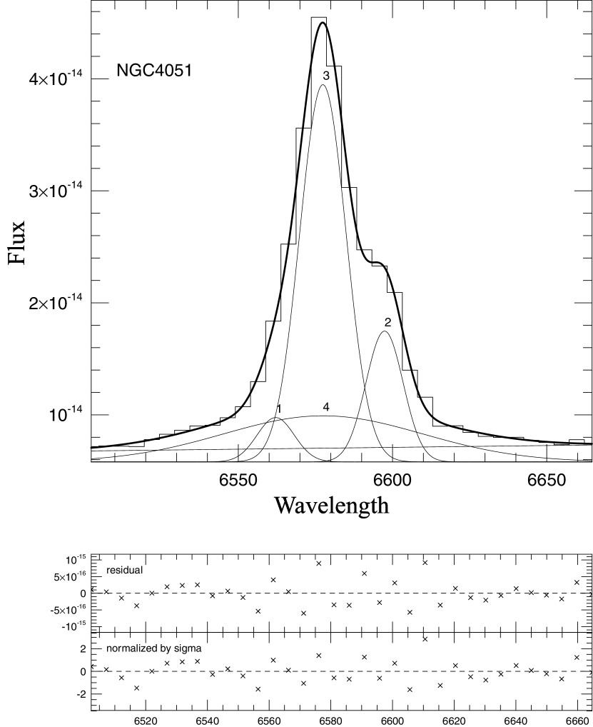
Figure 3.— Result of multi-Gaussian component fitting for the H$\alpha+$ [N II] emission lines of NGC 4051. The wavelength is shown in unit of ${\rm\AA}$, and the flux is shown in unit of erg cm^-2 sec${}^{-1}{\rm\AA}$.

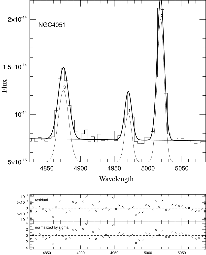
Figure 4.— Result of multi-Gaussian component fitting for the H$\beta+$ [O III] emission lines of NGC 4051. The unit for each axis is the same as Figure 3.

3.2. Spatial Distribution of the Emission-Line Region

In Table 3a – 3d, we give the emission-line properties of the off-nuclear regions; west (2$\farcs$9 west), southeast (1$\farcs$5 south 2″west), southwest (1$\farcs$5 south 2″east), and east (2$\farcs$9 east). Since the flux of [O I] $\lambda$6300 in these areas is not measured because of the insufficient S/N, we do not subtract the flux of [O I] $\lambda$6364 from that of [Fe X] $\lambda$6374. Though we measured the fluxes of emission lines of northeast, those data are not tabulated because we could not detect the H$\beta$ unambiguously. The S/N of the northwest position is so poor that we did not measure the fluxes of emission lines.

Table 3aEmission-Line Data of the Off-Nuclear Region (2$\farcs$9 west)

Identification	$\lambda_{{\rm obs}}$	FWHM	F/F(H$\beta$N)		I/I(H$\beta$N)
	(${\rm\AA}$)	(km s-1)	Line Ratios	1 $\sigma$	Line Ratios	1 $\sigma$
H$\beta$N	4874.8	677.1	1.000	—–	1.000	—–
[O III]	4970.7	657.9	0.563	$\pm$0.068	0.548	$\pm$0.066
[O III]	5018.7	651.6	1.660	$\pm$0.115	1.594	$\pm$0.111
[Fe X]	6391.2	765.9	0.680	$\pm$0.075	0.488	$\pm$0.061
[N II]	6562.6	771.2	0.634	$\pm$0.075	0.442	$\pm$0.059
H$\alpha$N	6577.3	769.5	4.440	$\pm$0.271	3.087	$\pm$0.268
[N II]	6597.9	767.1	1.870	$\pm$0.128	1.296	$\pm$0.120
[S II]	6733.0	—–	0.268	$\pm$0.053	0.182	$\pm$0.038
[S II]	6747.4	—–	0.405	$\pm$0.056	0.274	$\pm$0.042

Table 3bEmission-Line Data of the Off-Nuclear Region (1$\farcs$5 south - 2″west)

Identification	$\lambda_{{\rm obs}}$	FWHM	F/F(H$\beta$N)		I/I(H$\beta$N)
	(${\rm\AA}$)	(km s-1)	Line Ratios	1 $\sigma$	Line Ratios	1 $\sigma$
H$\beta$N	4869.4	839.7	1.000	—–	1.000	—–
[O III]	4967.1	444.6	0.459	$\pm$0.031	0.443	$\pm$0.030
[O III]	5015.1	440.3	1.353	$\pm$0.052	1.285	$\pm$0.049
He I	5886.6	832.6	0.226	$\pm$0.035	0.166	$\pm$0.026
[Fe X]	6381.2	705.4	0.244	$\pm$0.027	0.159	$\pm$0.018
[N II]	6559.5	666.9	0.616	$\pm$0.032	0.388	$\pm$0.024
H$\alpha$N	6574.2	665.4	4.911	$\pm$0.160	3.083	$\pm$0.143
[N II]	6594.8	663.3	1.819	$\pm$0.064	1.137	$\pm$0.055
[S II]	6731.1	—–	0.212	$\pm$0.022	0.129	$\pm$0.014
[S II]	6745.5	—–	0.185	$\pm$0.021	0.112	$\pm$0.014

Table 3cEmission-Line Data of the Off-Nuclear Region (1$\farcs$5 south - 2″east)

Identification	$\lambda_{{\rm obs}}$	FWHM	F/F(H$\beta$N)		I/I(H$\beta$N)
	(${\rm\AA}$)	(km s-1)	Line Ratios	1 $\sigma$	Line Ratios	1 $\sigma$
H$\beta$N	4870.8	1220.2	1.000	—–	1.000	—–
[O III]	4967.0	589.4	0.406	$\pm$0.056	0.394	$\pm$0.055
[O III]	5015.0	583.8	1.196	$\pm$0.091	1.145	$\pm$0.087
[N II]	6559.4	674.7	0.627	$\pm$0.054	0.425	$\pm$0.045
H$\alpha$N	6574.2	673.2	4.566	$\pm$0.290	3.086	$\pm$0.279
[N II]	6594.7	671.1	1.849	$\pm$0.122	1.245	$\pm$0.115
[S II]	6729.7	—–	0.245	$\pm$0.027	0.161	$\pm$0.021
[S II]	6744.1	—–	0.287	$\pm$0.029	0.189	$\pm$0.023

Table 3dEmission-Line Data of the Off-Nuclear Region (2$\farcs$9 east)

Identification	$\lambda_{{\rm obs}}$	FWHM	F/F(H$\beta$N)		I/I(H$\beta$N)
	(${\rm\AA}$)	(km s-1)	Line Ratios	1 $\sigma$	Line Ratios	1 $\sigma$
H$\beta$N	4871.1	781.7	1.000	—–	1.000	—–
[O III]	4968.5	517.5	0.995	$\pm$0.148	0.979	$\pm$0.146
[O III]	5016.5	512.6	2.936	$\pm$0.338	2.864	$\pm$0.332
[N II]	6560.7	607.2	0.739	$\pm$0.132	0.594	$\pm$0.126
H$\alpha$N	6575.5	605.8	3.852	$\pm$0.436	3.092	$\pm$0.498
[N II]	6596.0	604.0	2.180	$\pm$0.261	1.747	$\pm$0.291

Figure 5 shows that the HINER traced by [Fe X] $\lambda$6374 is extended westward up to 3″ ($\approx$ 150 pc). This is more extended than the NLR traced by [O I] $\lambda$6300. Since, as shown in Figure 6, there is no strong line of sky emission at the observed wavelength of [Fe X], the extended [Fe X] appears to be real. Figure 5 also shows that the HINER may be extended southwestward. However this may be due to the contamination from the nuclear region, suggested by the relatively broad width of H$\beta$ at the southwest position.

Following Veilleux & Osterbrock (1987), we investigate the excitation conditions of the emission-line region in each position. As shown in Figure 7, we find that the regions where [Fe X] is absent exhibit AGN-like excitations, whereas the regions where [Fe X] is found show H II region-like excitations (except for the southeast region where the line ratios show H II region-like excitation though [Fe X] is not detected). It is unlikely that the [Fe X] emission arises from H II regions. Therefore the observed H II region-like excitations are due not to photoionization by massive stars but to some additional mechanism. We will discuss this complex property in section 5.

Figure 5.— Extended HINER in NGC4051. These spectra are enlarged among [Fe X]. The numbers in parenthesizes show the offsets from the center of NGC4051 for each positions (written in unit of arcsecond).

Figure 6.— Nightglow spectrum. This spectrum is not calibrated for sensitivity of the detector. The numbers in this figure are the observed wavelength of each emission line of the nightglow in unit of angstrom.

Figure 7.— A diagnostic diagram of [O III]/H$\beta$ vs.[N II]/H$\alpha$ for NGC 4051. These line ratios are not corrected for reddening. The curve shows the distinction between AGN-like excitation and H II region-like excitation taken from Veilleux & Osterbrock (1987). The crosses shows the estimated 1 $\sigma$-level errors. The arrow means that the indicated line ratio of [O III]/H$\beta$ is the lower limit.

3.3. A Summary of the Observational Results

As noted in section 1, there are three kinds of the HINER; 1) the torus HINER, 2) the NLR HINER, and 3) the extended HINER (see MT98a). Our detection of the extended [Fe X] emitting region tells us that the extended HINER exists at least in NGC 4051. Here we estimate how strong the contribution from the torus HINER using the dual component photoionization model of MT98b. According to the diagnostic diagram of their model (Figure 2 in MT98b), we find that the torus HINER may contribute to the total intensity of the HINER emission less than 3%. On the other hand, if [Fe X] in the nuclear region was mainly attributed to the NLR HINER, this line would have a larger FWHM in the nuclear region than in off-nuclear regions because the flux contribution of the NLR HINER may be negligibly small in the off-nuclear regions. Since we could not find the difference of FWHM of [Fe X] between the nuclear region and west, the NLR HINER is not a dominant source in NGC 4051. It is therefore suggested that the majority of the HINER emission in NGC 4051 arises from low-density ISM within a radius of $\approx$ 150 pc.

4. PHOTOIONIZATION MODEL

In order to understand the nuclear environment of NGC 4051, we use photoionization models and compare the predictions of the models with the observed emission-line ratios of the nuclear region of NGC 4051. The simplest model for the NLRs of Seyfert galaxies is a so-called one-zone model, which assumes optically thick clouds of single density and single distance from the source of the ionization radiation (e.g. Ferland & Netzer 1983, Stasinska 1984). However, these models have been known to predict too weak high-ionization emission lines such as [Fe VII] $\lambda 6087$ and [Fe X] $\lambda 6374$, and moreover, predict less intense [Fe X] $\lambda$6374 than [Fe VII] $\lambda$6087. Because these model predictions appear inconsistent with observations, one-zone models are not suitable to investigate the environment of the nuclear region of NGC 4051. Hence, it is better to use more realistic models, for example, the optically-thin, multi-cloud model (Ferland & Osterbrock 1986) or the LOC models (Ferguson et al. 1997a). The predicted emission-line flux calculated with these models are shown in Table 4. The former model predicts [Fe VII] $\lambda$6087/[Fe X] $\lambda$6374 $\approx$ 10, that is inconsistent with the result of observations of NGC 4051. The LOC model also predicts [Fe X] $<$ [Fe VII]. Taking these points into accounts, we construct a two-component photoionization model below.

Table 4Model Predictions for Forbidden Lines

Line	FO86, optically thin	FKBF97, LOC model
		(Solar Abundance)	(Dusty Abundance)
[Ne V] $\lambda$3426	0.09	0.62	0.67
[O III] $\lambda$5007	7.11	11.7	10.8
[Fe XIV] $\lambda$5303	—	0.033	0.004
[Fe VII] $\lambda$6087	0.02	0.049	0.009
[O I] $\lambda$6300	0.85	0.56	0.84
[Fe X] $\lambda$6374	0.002	0.015	0.002
[N II] $\lambda$6583	2.56	1.18	1.69
[S II] $\lambda\lambda$6716+6731	1.37	1.20	1.87
[Fe XI] $\lambda$7892	—	0.068	0.008

4.1. A Two-Component Photoionization Model

We construct a two-component system for the nuclear emission-line region of NGC 4051. One component is optically thick, ionization-bounded clouds (IB clouds). This component emits low-ionization emission lines mainly, like clouds in typical NLRs. The other is optically thin, low-density, matter-bounded clouds (MB clouds; Viegas-Aldrovandi 1988; Viegas-Aldrovandi & Gruenwald 1988; Binette, Wilson, & Storchi-Bergmann 1996; Wilson, Binette, & Storchi-Bergmann 1997; Binette et al. 1997) which radiates high-ionization emission lines selectively. These MB clouds are expected to emit more intense [Fe X] $\lambda$6374 than [Fe VII] $\lambda$6087 because their densities are assumed to be low enough to achieve very high-ionization conditions (section 4.2).

Ionization and thermal equilibrium calculations have been performed with the photoionization code CLOUDY (version 90.04; Ferland 1996) to calculate the emission from plane-parallel, fixed hydrogen density clouds. Taking into account many lines of evidence in favor of a nitrogen overabundance (Storchi-Bergmann & Pastoriza 1990; Storchi-Bergmann 1991; Storchi-Bergmann et al. 1998), we adopt twice the solar nitrogen abundance. Namely, all elements have solar values except for nitrogen. The detection of strong [Fe X] suggests that most of iron remains in gas phase although the depletion of iron would be more serious than that of other elements (e.g., Phillips, Gondhalekar, & Pettini 1982). Therefore internal dust grains in the NLR are not taken into account in our calculations. The shape of the ionizing continuum from the central engine is

$$f_{\nu}=\nu^{\alpha_{{\rm uv}}}\exp(-\frac{h\nu}{kT_{{\rm BB}}})\exp(-\frac{kT_{{\rm IR}}}{h\nu})+a\nu^{\alpha_{{\rm x}}}.$$ (1)

We adopt the following parameters; (1) $kT_{\rm IR}$ is the infrared cutoff of the so-called big blue bump component and we adopt $kT_{\rm IR}$ = 0.01 Ryd; (2) $T_{\rm BB}$ is the temperature which parameterize the big blue bump continuum, and we adopt a typical value, $1.5\times 10^{5}$ K; (3) $\alpha_{\rm uv}$ is the slope of the low energy big blue bump component. We adopt $\alpha_{\rm uv}=-0.5$. Note that the photoionization is not sensitive to this parameter. And, (4) $\alpha_{\rm x}$ is the slope of the X-Ray component, and we adopt $\alpha_{\rm x}=-1.0$. This power law component is not extrapolated below 1.36 eV or above 100 keV. Below 1.36 eV, this term is set to zero while above 100 keV, the continuum is assumed to fall off as $\nu^{-3}$. Finally, (5) the UV to X-Ray spectral slope, $\alpha_{\rm ox}$, is defined as

$$\alpha_{{\rm ox}}\equiv\frac{\log[F_{\nu}({\rm 2keV})/F_{\nu}(2500{\rm\AA})]}{\log[\nu({\rm 2keV})/\nu(2500{\rm\AA})]},$$ (2)

which is a free parameter related to the parameter a in equation (1). We adopt $\alpha_{\rm ox}=-1.4$. The observational values of these parameters for NGC 4051 are summarized in Table 5.

Table 5Observational Constraint for Input Continuum

parameter	observational value	adopted value
TBB	—	1.5 $\times$ 105
$\alpha_{uv}$	—	–0.5
$\alpha_{x}$	–1.88$\pm$0.18  (ROSAT)	–1.0
	–0.66  (Ginga)
	–0.85$\pm$0.07  (ASCA)
	–1.30  (ROSAT)
$\alpha_{ox}$	–1.32  (ROSAT)	–1.4

The calculations for IB clouds are proceeded until the electron temperature drop below 3000 K, since the gas with lower temperature than 3000 K is not thought to contribute significantly to the emission lines. The calculations for MB clouds are proceeded till the column density of the MB clouds reach to a value given as a free parameter.

4.2. Results

First, we discuss the physical conditions of the IB clouds. Assuming that the low-ionization forbidden lines are radiated mainly from the IB clouds, we estimate the hydrogen density of the IB cloud $n_{\rm IB}$ = 10^2.9 cm^-3, which derived from the observed [S II] doublet ratio, [S II] $\lambda$6716/[S II] $\lambda$6731 = 0.934 (see Osterbrock 1989). Similarly, assuming that the MB clouds contribute to the flux of the low-ionization lines very little, we search an ionization parameter for the IB clouds, $U_{\rm IB}=Q({\rm H})/(4\pi R^{2}N_{\rm H,IB}c)$ (the ratio of the ionizing photon density to the Hydrogen density) using CLOUDY. Emission-line ratios of [O I] $\lambda$6300/[O III] $\lambda$5007, [N II] $\lambda$6583/[O III] $\lambda$5007 and [S II] $\lambda\lambda$6717,6731/[O III] $\lambda$5007 are calculated for various values of $U_{\rm IB}$, and compared with the observed values. As shown in Figure 8, the comparisons for the individual line ratios do not give a certain value of $U_{\rm IB}$. Therefore, we use the [S II] $\lambda\lambda$6717,6731/[O III] $\lambda$5007 ratio to determine the hydrogen density of the IB clouds, and then we derive $U_{\rm IB}$ = 10^-2.9 accordingly.

Second, we estimate most probable values of the parameters for MB clouds. When $U_{\rm MB}\geq$ 10^-0.4, the calculated flux of [Fe X] $\lambda$6374 is smaller than that of [Fe XI] $\lambda$7892; and when $U_{\rm MB}\leq$ 10^-0.6, [O III] $\lambda$5007 begins to emit from MB clouds. Because these conditions are not suitable to explain the observations, we adopt $U_{\rm MB}=10^{-0.5}$. When the hydrogen column density of MB clouds $N_{\rm MB}>10^{21}$ cm^-2, [O III] $\lambda$5007 also begins to radiate from the MB clouds (see Figure 9). Therefore we examine two cases for $N_{\rm MB}=10^{20.5}$ cm^-2 and for 10^21.0 cm^-2. Assuming the size of HINER $D_{\rm HINER}=150{\rm pc}=4.63\times 10^{20}$ cm, we obtain $n_{\rm MB}\simeq 10^{-0.17}$ cm^-3 for $N_{\rm MB}=10^{20.5}$ cm^-2 and $n_{\rm MB}\simeq 10^{0.33}$ cm^-3 for $N_{\rm MB}=10^{21}$ cm^-2 because $n_{\rm MB}\simeq N_{\rm MB}/D_{\rm HINER}$. Since the former density is too low to produce sufficiently strong emission, we adopt the latter case, that is, $n_{\rm MB}=10^{0.33}$ cm^-3 and $N_{\rm MB}=10^{21}$ cm^-2. In Table 6, we give the emission line fluxes normalized by H$\beta$ (narrow component) for the IB and MB clouds described above.

Table 6Observed and Calculated Line Ratios

Line	Observed	IB Clouds	MB Clouds
H$\beta$N $\lambda$4861	1.000	1.000	1.000
[O III] $\lambda$5007	1.294	3.937	0.114
[Fe XIV] $\lambda$5303	$<$ 0.063	0.000	0.160
He I $\lambda$5876	0.130	0.141	0.001
[Fe VII] $\lambda$6087	$<$ 0.060	0.000	0.014
[O I] $\lambda$6300	0.113	0.091	0.000
[Fe X] $\lambda$6374	0.136	0.000	2.658
H$\alpha$N $\lambda$6563	3.030	2.901	2.706
[N II] $\lambda$6584	0.838	2.200	0.000
[S II] $\lambda$6716	0.127	0.405	0.000
[S II] $\lambda$6731	0.136	0.441	0.000
[Fe XI] $\lambda$7892	$\cdots$	0.000	1.784

It seems reasonable that the nuclear emission-line region of NGC 4051 is a mixture of both IB and MB clouds. In order to reproduce the observed [Fe X]/H$\beta$ ratio, we find that the relative contribution of the MB clouds is 5.3% in the H$\beta$ luminosity. We compare the total calculated line ratios with the observed values in Table 7. We find that [O III], [N II] and [S II] are two or three times stronger than the observational values although high-ionization lines are consistent with the observation. This discrepancy can be reconciled if there is another emission component which radiates hydrogen recombination lines mainly. Hereafter we call this “contamination component”. Possible contamination sources are either BLR or nuclear star forming regions or both (section 5). Note that this contamination component must not destroy the line ratios such as $\lambda\lambda$6717,6731/[O III] $\lambda$5007, [S II] $\lambda$6716/[S II] $\lambda$6731 and so on.

Table 7Comparison of Calculated Line Ratios  IB+MB Model with Observed Values

Line	IB clouds	MB clouds	Total	Observed
H$\beta$N $\lambda$4861	0.947	0.053	1.000	1.000
[O III] $\lambda$5007	3.728	0.006	3.734	1.294
[Fe XIV] $\lambda$5303	0.000	0.008	0.008	$<$ 0.063
He I $\lambda$5876	0.134	0.000	0.134	0.130
[Fe VII] $\lambda$6087	0.000	0.001	0.001	$<$ 0.060
[O I] $\lambda$6300	0.086	0.000	0.086	0.113
[Fe X] $\lambda$6374	0.000	0.141	0.141	0.136
H$\alpha$N $\lambda$6563	2.747	0.143	2.890	3.030
[N II] $\lambda$6584	2.083	0.000	2.083	0.838
[S II] $\lambda$6716	0.384	0.000	0.384	0.127
[S II] $\lambda$6731	0.418	0.000	0.418	0.136
[Fe XI] $\lambda$7892	0.000	0.095	0.095	$\cdots$

Flux contributions of the IB clouds, the MB clouds, and the contamination component to Balmer lines are treated as free parameters a and b; a is the H$\beta$ flux ratio between the MB clouds and the IB clouds and b is that between the contamination component and the IB clouds. We can find a probable set of the line ratios which is consistent with the observation. Here we assume a ratio of H$\alpha$/H$\beta$ for the contamination component to be 3.1. Because [Fe X] is assumed to emit from the MB clouds, we obtain a relation:

$$(\frac{[{\rm Fe~{}X}]}{{\rm H}\beta})_{\rm obs}\ =\ \frac{a\times(\frac{[{\rm Fe~{}X}]}{{\rm H}\beta})_{\rm MB}}{1+a+b}.$$ (3)

Since we can regard [O III] $\lambda$5007 as a representative low-ionization emission line, we obtain another relation:

$$(\frac{[{\rm O~{}III}]}{{\rm H}\beta})_{\rm obs}\ =\ \frac{(\frac{[{\rm O~{}III}]}{{\rm H}\beta})_{\rm IB}}{1+a+b}.$$ (4)

In Table 6, we give ([Fe X]/${\rm H}\beta$)_obs, ([Fe X]/${\rm H}\beta$)_MB, ([O III]/${\rm H}\beta$)_obs, and ([O III]/${\rm H}\beta$)_IB. Using these relations, we find a = 0.161 and b = 1.868. These results mean that the contributions of the IB clouds, the MB clouds and the contamination component are 33.0%, 5.3% and 61.7% in the H$\beta$ luminosity, respectively. We give a summary of the set of the line ratios in Table 8. Though we do not observe [Fe XI] $\lambda$7892, previous observations (Penston et al. 1984 and Erkens et al. 1997) show [Fe XI] $\lambda$7892/[Fe X] $\lambda$6374 = 0.324 or 0.514. Our calculated [Fe XI] $\lambda$7892/[Fe X] $\lambda$6374 is 0.674, and this is not so different from the previous observations. On the other hand, the observed [O I] $\lambda$6300 is four times stronger than the model value. One reason for this may be that [O I] arises partly from other regions that we do not take into account in our model.

Table 8Comparison of Calculated Line Ratios  of Contaminated Model with Observed Values

Line	IB clouds	MB clouds	Contamination	Total	Observed
H$\beta$N $\lambda$4861	0.330	0.053	0.617	1.000	1.000
[O III] $\lambda$5007	1.299	0.006	0.000	1.305	1.294
[Fe XIV] $\lambda$5303	0.000	0.008	0.000	0.008	$<$ 0.063
He I $\lambda$5876	0.047	0.000	0.000	0.047	0.130
[Fe VII] $\lambda$6087	0.000	0.001	0.000	0.001	$<$ 0.060
[O I] $\lambda$6300	0.030	0.000	0.000	0.030	0.113
[Fe X] $\lambda$6374	0.000	0.141	0.000	0.141	0.136
H$\alpha$N $\lambda$6563	0.960	0.143	1.913	3.016	3.030
[N II] $\lambda$6584	0.726	0.000	0.000	0.726	0.838
[S II] $\lambda$6716	0.134	0.000	0.000	0.134	0.127
[S II] $\lambda$6731	0.146	0.000	0.000	0.146	0.136
[Fe XI] $\lambda$7892	0.000	0.095	0.000	0.095	$\cdots$

Finally, in Table 9, we give a summary of the three emission components adopted for the nuclear emission-line region of NGC 4051. These parameters are determined uniquely in the process described above. However, there may be other models which explain the observed line ratios of NGC 4051. Recently, Contini & Viegas (1999) proposed a multi-cloud model in which the existence of shocks is introduced for NGC 4051. Their model explains the optical line ratios and the continuum SED, although they did not mention the spatial extension of ionized regions. In order to discriminate which model is more plausible, further detailed observations will be necessary.

Table 9Properties of Each Component

	nH	U	NH	Contribution to H$\beta$
	(cm-3)		(cm-2)
IB clouds	102.9	10-2.9	—	33.0%
MB clouds	100.33	10-0.5	1021.0	5.3%
Contamination	$\cdots$	$\cdots$	$\cdots$	61.7%

Figure 8.— Determination of the parameters for ionization-bounded clouds. The straight lines show the observed reddening-corrected line ratios and the curves show the calculated line ratio for various parameters (here, hydrogen density and ionization parameter). The small circles are located at the crossover for the lines describing the observed and calculated line ratios, therefore the circles indicate the estimated parameters.

Figure 9.— Determination of the parameters for matter-bounded clouds. The curves show the calculated fluxes normalized by H$\beta$ for the varying hydrogen column density in the case of log U = –0.6, –0.5 and –0.4.

5. DISCUSSION

As we have shown in previous sections, the observed emission-line ratios of the nuclear region of NGC4051 are consistently understood by introducing the three emission components; 1) the ionization-bounded clouds, 2) matter-bounded clouds, and 3) the contamination component to the Balmer emission lines. Although our three-component model appears consistent with the observation, our result implies that the majority of Balmer emission ($\sim$ 60%) arises from the contamination component. Now we consider the problem; What is the contamination component ?

First, we consider this problem for the nuclear region. Possible candidates of the contamination components are either the BLR or nuclear star-forming regions or both. If NGC 4051 belongs to a class of NLS1s (Boller et al. 1996; Komossa & Fink 1997), it seems hard to measure the contribution from the BLR to the H$\beta$ emission because of the narrow with of the broad line if present. It is also possible to consider that NGC 4051 experiences a burst of massive star formation in its nuclear region because there is a lot of cold molecular gas as well as circumnuclear star-forming regions in NGC 4051 (Kohno 1997; Vila-Vilaró, Taniguchi, & Nakai 1998). Peterson, Crenshaw, & Meyers (1985) reported that H$\beta$ of NGC 4051 exhibits time variability (enhanced by 85% in H$\beta$ flux) on time scales shorter than $\sim$2 years, that is, H$\beta$ of NGC4051 contains the broad component more or less. Although we have no way to evaluate the contribution of this BLR contamination to the total flux quantitatively, it is possible that all of the contamination component is contributed from the BLR. In addition, the nuclear star-formation may contribute to the contamination. Kohno (1997) discussed the gravitational instability of the nuclear molecular gas of some Seyfert galaxies using the Toomre’s Q-value. The Toomre’s Q parameter characterizes the criterion for local stability in thin isothermal disks and is expressed as Q = $\Sigma_{{\rm crit}}/\Sigma_{{\rm gas}}$, where $\Sigma_{{\rm crit}}$ is the critical surface density. He gave Q = 0.90 for the nuclear region of NGC4051. This means that the molecular gas in the nuclear region of NGC4051 is thought to be gravitationally unstable.

In any case, about 60% of observed H$\beta$ is not originated from the NLR in the nuclear region of NGC 4051. This means that the line ratios of the nuclear region suffer seriously from the contamination. In Figure 10, we replot the excitation diagnostic diagram using the line ratios, from which the contamination component is subtracted. This diagram shows that the contamination-subtracted line ratios of nuclear region show the typical AGN-like excitation condition. Therefore we conclude that the unusual excitation condition is due to the contamination component. High-spatial resolution optical spectroscopy or X-ray imaging observations will be helpful in investigating whether or not the star-formation activity dominates the flux of H$\beta$.

Second, we consider the off-nuclear regions. As shown in Figure 7, the three off-nuclear regions (west, southwest, and southeast) also show H II region-like excitations. Since a typical size of the BLR is $\sim$ 0.01 pc (e.g. Peterson 1997), it is likely that these excitation conditions are thought to be due to circumnuclear star-forming regions.

Figure 10.— A diagnostic diagram samely as Figure 6. The filled circle shows the excitation condition of the nuclear region corrected for the contamination effect.

References

- (1) Adams, T. F. 1977, ApJS, 33, 19
- (2) Anderson, K. S. 1970, ApJ, 162, 743
- (3) Antonucci, R. R. J. 1993, ARA&A, 31, 473
- (4) Antonucci, R. R. J., & Miller, J. S. 1985, ApJ, 297, 621
- (5) Binette, L. 1985, A&A, 143, 334
- (6) Binette, L., Wilson, A., Rega, A., & Storchi-Bergmann, T. 1997, A&A, 327, 909
- (7) Binette, L., Wilson, A. S., & Storchi-Bergmann, T. 1996, A&A, 312, 365
- (8) Boller, Th., Brandt, W. N., & Fink, H. 1996, A&A, 305, 53
- (9) Contini, M., & Viegas, S. M. 1999, ApJ, 523, 114
- (10) De Robertis, M. M., & Osterbrock, D. E. 1986, ApJ, 301, 727
- (11) Erkens, U., Appenzeller, I., & Wagner, S. 1997, A&A, 323, 707
- (12) Ferguson, J. W., Korista, K. T., Baldwin, J. A., & Ferland G. J. 1997a, ApJ, 487, 122
- (13) Ferguson, J. W., Korista, K. T., & Ferland G. J. 1997b, ApJS, 110, 287
- (14) Ferland, G. J. 1996, HAZY: A Brief Introduction to CLOUDY (Univ. Kentucky Dept. Physics & Astron. Internal Rep.)
- (15) Ferland, G. J., & Osterbrock, D. E. 1986, ApJ, 300, 658
- (16) Ferland, G. J., & Netzer, H. 1983, ApJ, 264, 105
- (17) Francis, P. J. 1993, ApJ, 407, 519
- (18) Grandi, S. A. 1978, ApJ, 221, 501
- (19) Golev, V., Yankulova, I., Bonev, T., & Jockers, K. 1995, MNRAS, 273, 129
- (20) Guainazzi, M., Mihara, T., Otani, C., & Matsuoka, M. 1996, PASJ, 48, 781
- (21) Halpern, J. P., & Steiner, J. E. 1983, ApJ, 269, L37
- (22) Kohno, K. 1997, Doctor’s thesis, Tokyo Univ.
- (23) Komossa, S., & Fink, H. 1997, A&A, 322, 719
- (24) Korista, K. T., & Ferland, G. J. 1989, ApJ, 343, 678
- (25) Kosugi, G., Ohtani, H., Sasaki, T., Koyano, H., Shimizu, Y., Yoshida, M., Sasaki, M., Aoki, K., & Baba, A. 1995, PASP, 107, 474
- (26) Murayama, T., & Taniguchi, Y. 1998a, ApJ, 497, L9 (MT98a)
- (27) Murayama, T., & Taniguchi, Y. 1998b, ApJ, 503, L115 (MT98b)
- (28) Murayama, T., Taniguchi, Y., & Iwasawa, K. 1998, AJ, 115, 460 (MTI98)
- (29) Nussbaumer, H., & Osterbrock, D. E. 1970, ApJ, 161, 811
- (30) Oke, J. B., & Sargent, W. L. W. 1968, AJ, 73, 895
- (31) Osterbrock, D. E. 1969, Astrophys. Lett., 4, 57
- (32) Osterbrock, D. E. 1989, Astrophysics of Gaseous Nebulae and Active Galactic Nuclei (San Francisco: Freeman)
- (33) Osterbrock, D. E., & Dahari, O. 1983, ApJ, 273, 478
- (34) Osterbrock, D. E., & Pogge, R. W. 1985, ApJ, 297, 166
- (35) Penston, M. V., Fosbury, R. A. E., Boksenberg, A., Ward, M. J., & Wilson, A. S. 1984, MNRAS, 208, 347
- (36) Peterson, B. M. 1997, An introduction to active galactic nuclei (Cambridge Univ. Press)
- (37) Peterson, B. M., Crenshaw, D. M., & Meyers, K. A. 1985, ApJ, 298, 283
- (38) Phillips, A. P., Gondhalekar, P. M., & Pettini, M. 1982, MNRAS, 200, 687
- (39) Pier, E. A., & Voit, M. G. 1995, ApJ, 450, 628
- (40) Seyfert, C. K. 1943, ApJ, 97, 28
- (41) Stasinska, G. 1984, A&A, 135, 341
- (42) Storchi-Bergmann, T. 1991, MNRAS, 249, 404
- (43) Storchi-Bergmann, T., & Pastoriza, M. G. 1990, PASP, 102, 1359
- (44) Storchi-Bergmann, T., Schmitt, H. R., Calzetti, D., & Kinney, A. L. 1998, ApJ, 115, 909
- (45) Ulvestad, J. S., & Wilson, A. S. 1984, ApJ, 285, 439
- (46) Veilleux, S. 1988, AJ, 95, 1695
- (47) Veilleux, S., & Osterbrock, D. E. 1987, ApJS, 63, 295
- (48) Viegas-Aldrovandi, S. M. 1988, ApJ, 330, L9
- (49) Viegas-Aldrovandi, S. M., & Contini, M. 1989, A&A, 215, 253
- (50) Viegas-Aldrovandi, S. M., & Gruenwald, R. B. 1988, ApJ, 324, 683
- (51) Vila-Vilaró, B., Taniguchi, Y., & Nakai, N. 1998, AJ, 116, 1553
- (52) Walter, R., Orr, A., Courvoisier, T. J. -L., Fink, H. H., Makino, F., Otani, C., & Wamsteker, W. 1994, A&A, 285, 119
- (53) Wilson, A. S., Binette, L., & Storchi-Bergmann, T. 1997, ApJ, 482, L131
- (54) Yee, H. K. C. 1980, ApJ, 241, 894
- (55) Zamorani, G., Henry, J. P., Maccacaro, T., Tananbaum, H., Soltan, A., Liebert, J., Stocke, J., Strittmatter, P. A., Weymann, R. J., Smith, M. G., & Condon, J. J. 1981, ApJ, 245, 357