Gravitational lensing as folds in the sky

Abstract

We revisit the gravitational lensing phenomenon using a new visualization technique. It consists in projecting the observers sky into the source plane, what gives rise to a folded and stretched surface. This provides a clear graphical tool to visualize some interesting well-known effects, such as the development of multiple images of a source, the structure of the caustic curves, the parity of the images and their magnification as a function of the source position.

1 Introduction

The gravitational bending of light gives rise to many exciting observable effects such as the multiple images of distant quasars, the distortion of faint background galaxies by foreground clusters or the microlensing of stars in the Milky Way and nearby galaxies. The different phenomena that gravitational lensing can produce have been widely studied and the field has developed to become a major tool to investigate several astrophysical problems, such as the determination of the Hubble constant, of the amount of dark matter in the Universe, of the amount of compact objects in the Milky Way, the search of planetary systems, etc. [1, 2, 3, 4, 5, 6].

When the lensing mass distribution is concentrated at some distance from the observer, e.g. if it belongs to a cluster along the line of sight to a quasar or if it is a compact astrophysical object (possibly a binary) along the line of sight to a star, one can talk about the thin lens approximation, in which the ‘lens plane’ is well defined. A vector lens equation describes the position of the images of a point source that is viewed through a distribution of matter acting as lens. When this mapping is not single valued, multiple images of the source arise, this is the so called strong lensing regime. For non-singular lenses, images appear and disappear in pairs [7] as the source crosses lines in the source plane called caustics. These caustics hence divide regions in the sky with different number of images. The images that appear or disappear as the source crosses a caustic have opposite parities.

Here we describe a method that allows to visualize these properties in a simple way and graphically determine the position of the caustics as well as the number of images for a given lens configuration. This consists in projecting the observer’s sky into the source plane using the lens equation. The surface describing the sky seen at Earth (the ‘sky sheet’) appears folded (if strong lensing occurs) and stretched in the source plane. The location of the foldings corresponds to the position of the caustics, along which the magnification of the images diverges. Every fold produces a pair of new images of the source with opposite parities. Foldings can be closed lines or they can end in a point called a cusp, where two foldings merge so that the sky sheet unfolds. If the lenses are singular, e. g. in the limit of point-like masses relevant for microlensing, a tear appears in the sky sheet and one of the new images is lost. This will be described in section 2 which is devoted to lensing by a single lens. For single lenses the circular symmetry produces a point like caustic when the lens is perfectly aligned with the source. We also describe in section 2 how this caustic is transformed when an external shear is added. Some binary lens cases are then analyzed in section 3.

2 The single lens

2.1 The lens equation

As a first example we consider a single lens, corresponding to a mass distribution located at a distance $D_{ol}$ from the observer, acting as lens for a source located at a larger distance $D_{os}$ (for cosmological distances the angular diameter distance has to be used). According to general relativity, light rays traversing the lens plane are deflected by an angle $\vec{\hat{\alpha}}$ that depends in general on the distance to the mass distribution. Thus, the images of a source located at an angular position $\vec{\beta}$ will appear at angular position(s) $\vec{\theta}$ satisfying the lens equation

$$\vec{\beta}=\vec{\theta}-\vec{\alpha}(\vec{\theta}),$$ (1)

where $\vec{\alpha}\equiv\vec{\hat{\alpha}}D_{ls}/D_{os}$ and $D_{ls}$ is the distance from the deflector to the source.

For a point mass lens, which is a good approximation for star lenses, the deflection angle is given by

$$\hat{\alpha}=\frac{4GM}{c^{2}\xi},$$ (2)

with $\xi$ being the distance to the lens from the point at which the light ray intersects the lens plane. The deflection angle points in the direction from that point to the lens. In terms of the Einstein angle, $\theta_{E}\equiv(4GMD_{ls}/c^{2}D_{ol}D_{os})^{1/2}$, the lens equation reduces in this case to

$$\vec{\beta}=\vec{\theta}\left(1-\frac{\theta_{E}^{2}}{\theta^{2}}\right),$$ (3)

where the angles are measured with respect to the direction towards the lens. This equation has two solutions for every value of $\vec{\beta}$, except for $\vec{\beta}=0$ (perfect source–lens alignment) where all the points along the circle $|\vec{\theta}|=\theta_{E}$ (Einstein’s ring) are images.

When the object acting as lens is a galaxy or a cluster, an extended mass distribution has to be considered. Different models have been proposed for this extended distribution [10]. A simple and widely used one, that reproduces the observed flat rotation curves of galaxies, is the singular isothermal sphere, which has a mass distribution given by $\rho(r)=\sigma^{2}/2\pi Gr^{2}$. Here $\sigma$ is the one-dimensional velocity dispersion, which is related to the rotational velocity by $v_{r}=\sqrt{2}\sigma$. This model leads to a deflection angle

$$\hat{\alpha}=4\pi\frac{\sigma^{2}}{c^{2}},$$ (4)

which is independent of the distance to the lens and points towards the center of the mass distribution. The Einstein angle in this case is given by

$$\theta_{E}=4\pi\frac{\sigma^{2}}{c^{2}}\frac{D_{ls}}{D_{os}},$$ (5)

and hence the lens equation can now be written as

$$\vec{\beta}=\vec{\theta}\left(1-\frac{\theta_{E}}{\theta}\right).$$ (6)

A source located inside the Einstein ring will have two images, one at an angle larger than $\theta_{E}$ and the other one at a smaller angle. If the source lies outside the Einstein ring it has just one image, while if it is aligned with the center of the distribution the image will be the Einstein ring.

The singularity in the center of the mass distribution can be smoothed by a core region with finite density given by

$$\rho(r)=\frac{\sigma^{2}}{2\pi Gr_{c}^{2}}\frac{3+(r/r_{c})^{2}}{[1+(r/r_{c})^{2}]^{2}},$$ (7)

the deflection angle becomes

$$\vec{\hat{\alpha}}=4\pi\frac{\sigma^{2}}{c^{2}}\frac{\vec{\theta}}{\sqrt{\theta^{2}+\theta_{c}^{2}}},$$ (8)

where $\theta_{c}\equiv r_{c}/D_{ol}$. The lens equation can be written in this case as

$$\vec{\beta}=\vec{\theta}\left(1-\sqrt{\frac{\theta_{E}^{2}+\theta_{c}^{2}}{\theta^{2}+\theta_{c}^{2}}}\right),$$ (9)

where the Einstein angle is

$$\theta_{E}=\sqrt{16\pi^{2}\frac{\sigma^{4}}{c^{4}}\frac{D_{ls}^{2}}{D_{os}^{2}}-\theta_{c}^{2}}.$$ (10)

This softened isothermal sphere has smoother behavior than the singular models and hence we will often adopt it as a reference model. In particular, it will be useful to discuss the formation of image pairs. The analytical solutions of the lens equation giving the position of the image(s) for a given source is trivial in the singular cases (eqns. (3) and (6)), but to obtain $\theta_{i}(\beta)$ (where $i$ labels the images) in the non–singular case requires to find the solution of the fourth order equation

$$\theta^{4}-2\beta\theta^{3}+(\beta^{2}-\theta_{E}^{2})\theta^{2}-2\theta_{c}^{2}\beta\theta+\beta^{2}\theta_{c}^{2}=0,$$ (11)

with the constraint sign$(\theta-\beta)=\$sign$(\theta)$. This last constraint eliminates one spurious solution of eq. (11), leaving only one or three physical solutions which correspond to the location of the images of the source.

2.2 The sky sheet

We turn now to the construction of the sky sheet corresponding to a given lens configuration. This is done by considering light rays which arrive to the observer along directions forming a regular grid (in $\vec{\theta}$) and following them back to the source plane according to the lens equation (1). The image of this grid will define a new surface in the source plane, which will be stretched and folded. This problem is two dimensional, i.e. it involves only the observers coordinates $(\theta_{x},\theta_{y})$ or the source coordinates $(\beta_{x},\beta_{y}$). However, to visualize the folds in the sky sheet we have assigned also a vertical coordinate $z$ to the mapping from the observer to the source skies. We have conveniently chosen this vertical coordinate as being proportional to the time delay between the actual path of the light of each image of a source located at $(\beta_{x},\beta_{y}$) and the straight path from a source located at $\vec{\beta}=0$ in the absence of lenses.

The time delay for light rays coming from a given source due to the presence of a lens has a geometrical contribution coming from the extra path length of the deflected ray, plus a gravitational contribution due to the time stretching in the gravitational potential

$$t(\theta)=\frac{(1+z_{l})}{c}\frac{D_{ol}D_{os}}{D_{ls}}\left(\frac{1}{2}\alpha^{2}(\vec{\theta})-\Psi(\vec{\theta})\right),$$ (12)

where we allowed for a finite redshift $z_{l}$ of the lens and $\Psi(\vec{\theta})$ is proportional to the projected gravitational potential of the lens on the lens plane,

$$\Psi(\vec{\theta})=\frac{D_{ls}}{D_{ol}D_{os}}\frac{2}{c^{2}}\int\Phi(D_{ol}\vec{\theta},z){\rm d}z,$$ (13)

with $\Phi$ the three-dimensional gravitational potential. $\Psi$ is scaled in such a way that the deflection angle is given by $\vec{\alpha}(\vec{\theta})=\vec{\nabla}_{\theta}\Psi$. This time delay is measured with respect to the arrival time from the same source in the absence of lenses. To better visualize the sky sheets we have found more convenient to use the time delay with respect to a source located at $\vec{\beta}=0$ as the $z$ coordinate. Taking the $z$ coordinate proportional to the time delay allows to display the arrival time ordering of the flux variations of the source for the different images, so that flux changes will first appear for the image with smaller $z$.

Notice that when the time delay is plotted as a function of $(\theta_{x},\theta_{y})$ for a fixed source position $\beta$, a surface of time delays is obtained whose extrema (maxima, minima and saddle points) give the position of the images of the source according to Fermat’s principle [11]. This surface should not be mistaken with our sky sheet, which is plotted as a function of $(\beta_{x},\beta_{y})$, i.e. for different source locations, and the height $z$ is associated with the time delay of the actual images.

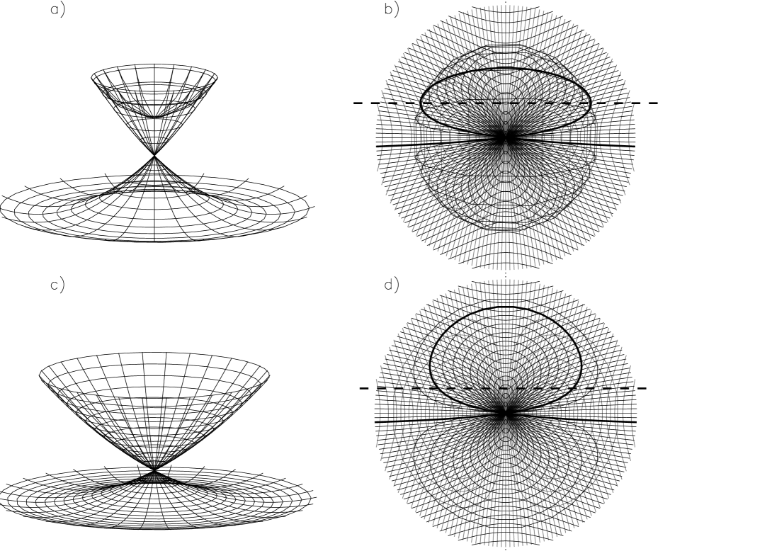
Figure 1: The sky sheet for the isothermal sphere. Panel a) displays the case of a softened isothermal sphere with a core radius $\theta_{c}=0.2~{}\theta_{E}$. The horizontal axes are the coordinates in the source plane $(\beta_{x},\beta_{y})$. The vertical axis is taken proportional to the time delay associated to each image. The number of images of a source is given by the times that a vertical line in the source location intersects the sky sheet. The order of arrival of a light pulse from the source is proportional to the $z$ coordinate and hence the image with smaller $z$ will show the pulse first. Panel b) shows a projection of case a) into the $(\beta_{x},\beta_{y})$ plane. The thick solid line displays the points observed in the source plane when we move the observation direction along a straight line. Panels c) and d) are similar to a) and b) but for the case of a singular isothermal sphere. Notice that the upper cap has disappeared in the singular case and the sky sheet is opened

Figure 1a shows this sky sheet for the case of the softened isothermal sphere. In this case a circularly symmetric fold develops, which looks like a blob in the surface. The horizontal coordinates are $(\beta_{x},\beta_{y}$), so that the number of intersections of the vertical lines with the surface give the number of images in the observer’s sky. Clearly for point sources located in the region covered by the blob, three images will be seen at three different positions in the sky, while for sources located outside the blob just one image will be seen. Figure 1b shows the projection of the sky sheet in the $(\beta_{x},\beta_{y})$ plane, i.e. as seen from above. The amplification of a given image is related to how much this surface is stretched at the point corresponding to the image (here we started with a rectangular grid so that the stretching can be visualized, while in Figure 1a and 1c we used a polar grid to respect the symmetry of the lens). If the surface is very stretched, the magnification is very low, while if it is contracted, the magnification is high. The circle corresponding to the border of the blob has then divergent magnification and corresponds to a caustic. When a source crosses it, a pair of new images appears in a different region of the sky, corresponding to the intersection of the vertical from the source position $(\beta_{x},\beta_{y}$) with the blob. This is a fold caustic according to the catastrophe theory classification [12, 13], and we see that it actually corresponds to a fold in the sky sheet. The other singular point is the central one, corresponding to the place where the blob formed. A source located there (i.e. perfectly aligned with the lens) will have as images all the points of the circle (i.e. the Einstein ring) that contracted to that point. This is a point-like caustic, which can appear exclusively for circularly symmetric lens configurations.

It is interesting to note that if we for instance point a telescope at a fixed latitude and move it from left to right along a meridian through a region of the sky where an isothermal lens is located, we are first seeing points in the source plane from left to right. When we arrive to the fold caustic, we start moving in the source plane from right to left as we move the telescope to the right, and the direction reverses again when we arrive to the other fold caustic. Thus, we cross the blob region three times, first to the right, then to the left and again to the right, as it is clear following the thick line in Figure 1b.

Figure 2: Sky sheet for the point-like lens

Figure 1c and 1d show the sky sheet for the case of the singular isothermal sphere. Here, the sky sheet develops a cut in the blob, transforming the blob into a cone, and the most demagnified central image disappears. Thus, a source can have just one or two images in this case. The second image appears or disappears as the source crosses the cut in the sky sheet and has its parity inverted (for instance, it is easy to see from the blob picture 1c which was drawn with polar coordinates, that the $\hat{\theta}$ unit vector will reverse orientation when projected into the source plane if it is inside the cone, while the unit vector in the radial direction will not be reversed, and hence the parity has to change).

For the point-like mass the deflection angle formally diverges as we approach the lens direction, thus in this case there is also a cut in the sky sheet, but the border is stretched to infinity, as shown in Figure 2. Hence, in this case there are always two images for any source position (except for perfect alignment, where the Einstein ring is the image). The principal image is always magnified, while the other one can become very demagnified, what is reflected here in that the conical surface becomes very stretched as we move out from the lens position.

Figure 3: Left panels: position of the images for a source moving along a straight line (dotted) with impact parameter $0.2~{}\theta_{E}$ for the softened isothermal sphere (top), the singular isothermal sphere (middle) and the point-like lens (bottom). The circles and squares identify the positions of the source and images for two different times. Right panels: amplification of the individual images (thin lines) as the source crosses the lens. The thick lines correspond to the sum of the amplifications.

The magnification of the images is given, in the case of circular symmetry considered, by $A_{i}=\left|\frac{\theta_{i}}{\beta}{\partial\theta_{i}\over\partial\beta}\right|$. The resulting expressions for the singular cases are well known, and for the non–singular case we have found the amplifications using the solutions $\theta_{i}(\beta)$ of eq. (11).

In Figure 3 we display illustrative examples for each of the three models. In the left panels we show the image locations (the axes are $(\theta_{x},\theta_{y}$), measured in units of the corresponding Einstein radii) for a source located at $\beta_{y}=0.2~{}\theta_{E}$ and with varying $\beta_{x}$, i.e. moving it along the dotted horizontal line. Two particular source positions and their images are identified with an asterisk and a square. From top to bottom the Figures correspond to the softened isothermal sphere, the singular isothermal sphere and the point-like mass. This corresponds to a source crossing the source plane along the dashed line in Figures 1b and 1d.

Figure 4: The sky sheet for a singular isothermal sphere with $\theta_{c}=0.2~{}\theta_{E}$ in the presence of an external shear corresponding to different values of $\gamma$.

In the right panels of Figure 3 we show for the same systems the corresponding magnifications $A_{i}$ as a function of $\beta_{x}$ (measured in units of $\theta_{E}$). The thin lines correspond to the individual images, while the thick lines indicate the sum of the amplifications, which is the relevant quantity when the images are unresolved. Notice that in the non singular case, the fainter image (dashed line in the first panel in Figure 3) is the one closest to the optical axis. Its magnification would decrease with decreasing core size $\theta_{c}$, becoming zero in the singular limit $\theta_{c}\to 0$ (this explains why only two images are seen in the singular cases, the two lower panels in Figure 3). Due to its significant demagnification, this third image is usually missed in the observations of multiple images of quasars. We also see that besides the high magnifications of the images for small $\beta$, there are now also peaks of high magnification associated to the formation or disappearance of the image pairs at caustic crossing, something that is not observed in the singular cases.

2.3 Distorting the point-like singularity

In the three examples illustrated the lens is circularly symmetric and hence they all have the point-like caustic in the center, whose image is the Einstein ring. Any departure from this lens symmetry will make the point-like caustic to distort to several fold caustics merging in pairs at cusps. For example, we could add to the smooth isothermal sphere an external shear $\gamma$ and convergence $\kappa$ to model the local effect of the environment around a lensing galaxy or an elliptical lens [15, 16]). This effect can be described by the first terms of the Taylor expansion of the projected gravitational potential, which in the principal axes system of the shear is

$$\Psi(\theta_{x},\theta_{y})=\frac{\kappa}{2}(\theta_{x}^{2}+\theta_{y}^{2})+\frac{\gamma}{2}(\theta_{x}^{2}-\theta_{y}^{2}),$$ (14)

A non-vanishing shear then clearly breaks the circular symmetry of the lens. For this case the lens equation can be written as

$$\beta_{x} = \theta_{x}\left(1-\kappa-\gamma-\frac{D_{ls}}{D_{os}}\frac{4\pi\sigma^{2}}{c^{2}}\frac{1}{\sqrt{\theta^{2}+\theta_{c}^{2}}}\right),$$ (15)

$$\beta_{y} = \theta_{y}\left(1-\kappa+\gamma-\frac{D_{ls}}{D_{os}}\frac{4\pi\sigma^{2}}{c^{2}}\frac{1}{\sqrt{\theta^{2}+\theta_{c}^{2}}}\right).$$ (16)

We show in Figure 4 the sky sheet for a set of values of $\gamma$ and $\kappa=0$. For small values of $|\gamma|$, such that $|\kappa\pm\gamma|<1$, the central point-like caustic is deformed to four fold caustics ending in four cusps. This can be understood as follows. In the circularly symmetric case, the Einstein ring was contracted to a point in the sky sheet, the point of contact of the blob with the rest of the surface. When we add a shear, there are for instance two different circles that will become shrinked to segments, one in the $\beta_{x}$ direction (with radius equal to the value of $\theta$ giving $\beta_{y}=0$ in eq. (15)), and the other in the $\beta_{y}$ direction (with radius equal to the value of $\theta$ giving $\beta_{x}=0$ in eq.  (16)). When identifying a circle with a segment, the interior of the circle will give rise to a blob, whose border will be a fold caustic. The endpoints of the above mentioned segments will correspond to the merging of two folds into a cusp. Depending on its location, a source can have one, three or five images. We have to count how many times the point at which the source is located is covered by the sky sheet. Points that are inside the oblate caustic (in the first two panels in Figure 4) get a pair of additional images and those that are inside the diamond shaped caustic get another additional pair.

If the value of the shear is increased, the structure of the caustics changes. The oblate caustic (pure fold) shrinks inside the diamond caustic, taking with it the pair of cusps which were in the horizontal direction (third panel of Figure 4). In this process the diamond shaped caustic has lost a pair of cusps and hence also appears as two folds merging into two cusps (this pair of cusps are far away in the vertical direction and thus are not displayed in the figure).

Figure 5: Close view of a cusp: two caustics merge and the sky sheet unfolds.

Figure 6: Different cuts of the sky sheet for the isothermal sphere with shear $\gamma=0.3$. The $z$ coordinate is proportional to the time delay associated to each image and gives the order of arrival of a pulse. In each line we indicate if the images along it correspond to a minimum (m), a saddle point (s) or a maximum (M) of the time delay function.

When $|\gamma|>1$, the vertical fold disappears (it is stretched to infinity) and only the horizontal fold shown in the last panel of Figure 4 remains. In this case there are just two folds merging into two cusps (lips singularity). A source inside the folds has three images, while one outside has one image. When a source crosses this lens in a direction transverse to the folds, a pair of new images adds to the original one in a different place of the sky when the source crosses the first folding. One of the new images is inverted, while the other is not. As the source continues moving, the inverted image approaches the original image, merges with it when the source crosses the second caustic and they disappear, leaving as single image of the source the one which was created in the crossing of the first fold. When the source enters the folded region through the cusp, the new pair of images appears in the same position as the original image, and then they separate from each other. We show in Figure 5 a close view of a cusp. It is clear how the two caustics, corresponding to the folds in the sky sheet, end in the cusp and the sky sheet surface unfolds there.

To better appreciate the folds in Figure 4 and the time delay structure of the images, we present in Figure 6 different vertical cuts of the second panel in Figure 4. The boxes show the sky sheet profiles along the indicated cuts which allow the visualization of the folds. We have also indicated the nature of the different images along each sheet, i.e. whether they are minima ($m$), saddle points ($s$) or maxima $(M)$ of the time delay function. These properties change at each fold of the sheet. The pair of images created in a fold can be a saddle point and a maximum or a saddle point and a minimum. The saddle points correspond to the images with inverted parities. The vertical coordinate we have chosen clearly allows a simple characterization of the extrema just by inspection of these cuts and knowing that far from the lens the single images are minima of the time delay. If the lens were to become singular, the sky sheet would be qualitatively similar except that the upper surface (the maximum) would be absent, leaving a hole in the sky sheet.

3 Binary lenses

Another configuration in which the circular symmetry is broken is when a second lens is present in the proximity of the original one. This configuration is of relevance for the study of microlensing by binary stars or planetary systems. When the lens is formed by a binary system, the deflection angle of a given light ray is given by the superposition of the deflections produced by the two individual lenses. If the lenses, that we take as softened isothermal spheres with dispersion velocities $\sigma_{1}$ and $\sigma_{2}$, are located in the lens plane forming angles $\vec{\theta}_{1}$ and $\vec{\theta}_{2}$ with the chosen optical axis, then the lens equation can be written as

$$\vec{\beta}=\vec{\theta}-\mu_{1}(\vec{\theta}-\vec{\theta}_{1})\sqrt{\frac{\theta_{E}^{2}+\theta_{c}^{2}}{|\vec{\theta}-\vec{\theta}_{1}|^{2}+\theta_{c}^{2}}}-\mu_{2}(\vec{\theta}-\vec{\theta}_{2})\sqrt{\frac{\theta_{E}^{2}+\theta_{c}^{2}}{|\vec{\theta}-\vec{\theta}_{2}|^{2}+\theta_{c}^{2}}}$$ (17)

where $\mu_{1}\equiv\sigma_{1}^{2}/\sigma^{2}$, $\mu_{2}\equiv\sigma_{2}^{2}/\sigma^{2}$, with $\sigma^{2}=\sigma_{1}^{2}+\sigma_{2}^{2}$, and $\theta_{E}$ refers to the Einstein angle of a single lens with velocity dispersion $\sigma$ (eq. 10)

Figure 7: The sky sheet for a binary lens composed of two identical softened isothermal spheres for different values of separation between the lenses.

The caustics for the case of two equal point-like lenses have been studied in detail by Schneider and Weiss [17]. An extension to more general geometries can be found in Refs. [18] and [19]. A numerical study of the extension to an ensemble of compact objects can be found in ref. [20].

We show in Figure 7 the sky sheet for the case of equal lenses ($\sigma_{1}=\sigma_{2}$) and an ensemble of values for the lens separation $\delta\equiv|\vec{\theta}_{1}-\vec{\theta}_{2}|/\theta_{E}$. We took for both lenses a core radius $\theta_{c}=0.2~{}\theta_{E}$. As the distribution of matter is smooth, there are no cuts in the sky sheet and the additional images appear in pairs (there is an odd number of them for every source position). If the distance between the lenses is large, the caustics associated to each lens are separated. Each one has a pure fold caustic and a diamond shaped caustic with four cusps. A source can have one, three or five images depending on whether it is located outside the caustics, inside either the fold or the diamond caustic, or inside both of them (first panel). As the lenses get closer, the diamond shaped caustics become more elongated, until they merge and form a six cusps caustic as shown in the second panel . For even closer lenses, the two pure fold caustics (the blobs) intersect and a region with seven images develops in the center (third panel). The fourth panel shows that as the lenses continue to approach each other the six cusps caustic shrinks to a four cusps caustic (actually, in an intermediate stage two small triangles are formed at the top and bottom of the diamond caustic in beak-to-beak singularities, and they shrink and disappear in a higher order catastrophe, leading to a single pure fold caustic containing a vertical lips singularity. This last shrinks and disappears for decreasing $\delta$, and the single lens caustics are recovered in the limit $\delta\to 0$).

Figure 8: The sky sheet for a binary lens composed of two softened isothermal spheres separated by a distance $\delta=1.2$ for different values of the mass ratio $\mu_{1}$.

It is straighforward to generalize this to an asymmetric case. As an example we show in Figure 8 the sky sheet for a binary lens system with different masses. We take two softened isothermal spheres with core radius given by $\theta_{c}=0.2~{}\theta_{E}$. The distance between the lenses is fixed at $\delta=1.2$, and the sky sheet is shown for different values of the parameter $\mu_{1}$. If one of the masses largely dominates the system, the sky sheet resembles the single lens case, but instead of the central point like caustic there is diamond shaped caustic. As the second mass becomes more important a new vertical fold starts to develop inside the diamond. This fold grows with the mass of the second lens and eventually cross the border of the diamond, transforming the diamond in a six cusps caustic and giving rise to a new pure fold caustic associated to the second lens (this transition is associated with two hyperbolic umbilics).

4 Conclusions

Some basic properties of simple gravitational lensing systems have been displayed using a graphical approach. This consists in projecting a regular grid in the image (observers) plane to the source plane using the lens equation. In the strong lensing regime, the mapping is not one to one, thus the regular grid becomes folded in the source plane.

This construction is straightforward and has several useful properties. In the first place, it gives a clear picture of which regions of the sky are seen when we look along directions close to a lensing system. The location of the caustics corresponds to the folds in the sky sheet. It is also easy to determine the number of images of a given source by counting the number of times that the sky sheet covers that position. The stretching of the sky sheet surface gives an idea of the magnification of each image.

The sky sheet plots provide also a simple pictorial view of features like the formation of additional images in pairs when the source crosses a caustic, of the parity of the images, or the fact that new images appear close to the original one when the source crosses a cusp.

Finally, the choice of the $z$ coordinate as proportional to the time delay associated to each image allows to display the ordering of arrival of any luminosity change of the source along the different image directions, and also to characterize the kind of extrema of the time delay function associated with each image.

Work partially supported by CONICET, Fundación Antorchas and Agencia Nacional de Promoción Científica y Tecnológica. We thank the CERN Theory Division for hospitality while part of this work was being done.

References

- [1] Blandford R. and Narayan R., ARAA 30, 311 (1992)
- [2] Schneider P., Ehler J. and Falco E., Gravitational Lenses, Springer Verlag, Berlin (1992)
- [3] Narayan R. and Bartelmann M., Lectures on Gravitational Lensing, astro-ph/9606001 (1996)
- [4] Paczynski B., ARAA 34, 419 (1996)
- [5] Roulet E. and Mollerach S., Phys. Rep. 279, 67 (1997)
- [6] Wambsganss J., astro-ph/9812021 (1998)
- [7] Burke W. L., ApJ 244, L1 (1981)
- [8] Gurevich A. V., Zybin K. P. and Sirota V. A., Phys. Lett. A 214, 232 (1996)
- [9] Zakharov A. F. and Sazhin M. V., JETP 83, 1057 (1996)
- [10] Hattori M., Kneib J.-P. and Makino N., astro-ph/9905009 (1999)
- [11] Blandford R. and Narayan R., ApJ 310, 568 (1986)
- [12] Berry M. V., Adv. Phys. 25, 1 (1976)
- [13] Poston T. and Stewart I. N., Catastrophe theory and its applications, London, Pitman (1978)
- [14] Virbhadra K. S. and Ellis G. F. R., astro-ph/9904193 (1999)
- [15] Chang K. and Refsdal S., A&A 132, 168 (1984)
- [16] Kovner I., ApJ 312, 22 (1987)
- [17] Schneider P. and Weiss A., A&A 164, 237 (1986)
- [18] Erdl H. and Schneider P., A&A 268, 453 (1993)
- [19] Dominik M., astro-ph/9903014 (1999)
- [20] Kayser R., Weiss A., Refsdal S. and Schneider P., A&A 214, 4 (1989)