Abstract

We present the evolution of magnetic nonpotentiality associated with an X-class flare in AR 6919 using a set of MSO (Mees Solar Observatory) magnetograms. The magnetogram data were obtained before and after the flare, using the Haleakala Stokes Polarimeter which provides simultaneous Stokes profiles of the Fe I doublet 6301.5 and 6302.5. A nonlinear least square method was adopted to derive the magnetic field configuration from the observed Stokes profiles and a multi-step ambiguity solution method was employed to resolve the $180^{\circ}$ ambiguity.

From the $180^{\circ}$ ambiguity-resolved vector magnetograms, we have derived a set of physical quantities characterizing the field configuration such as vertical current density, magnetic shear angle, angular shear and magnetic free energy density. We have examined their changes before and after the flare occurrence and obtained the following results. 1) There was a flux decrease in both polarities around a $\delta$-type sunspot region, where an X-class flare occurred. 2) The vertical current near the $\delta$ sunspot region was strongly enhanced before the flare. 3) The magnetic shear near the $\delta$ sunspot region increased before the flare and then decreased after it. 4) The sum of magnetic energy density significantly decreased before the flare onset, implying that magnetic free energy was released through the flaring processes.

Section 1 Introduction

It is generally believed that the energy released in solar flares is stored in nonpotential magnetic fields. The energy buildup could be a response of the coronal magnetic field to the changes in photospheric magnetic environment caused mostly by sunspot motions and emerging fluxes. Since the measurement of magnetic fields in the corona is not available, the field measurement at the photospheric level has been widely used for the study of magnetic nonpotentiality in flare-producing active regions. In particular, the change of some nonpotentiality parameters during flare activity is regarded as a very important clue for understanding flare mechanisms.

The MSFC (Marshal Space Flight Center) group studied the magnetic nonpotentiality associated with solar flares using the MSFC magnetograph (Hagyard et al., 1982; Hagyard et al., 1984). They examined the vertical current density, source field and magnetic shear derived from vector magnetograms of active regions in parallel with flare observations (Hagyard et al., 1984; Gary et al., 1987; Hagyard et al., 1990). On the basis of these studies, they suggested a few important points characterizing flare producing active regions. They are a large shear angle, a strong transverse magnetic field along the neutral line and a twist of long neutral lines (Gary et al., 1991). The BBSO (Big Bear Solar Observatory) and Huairou (Beijing Observatory) groups have also presented several interesting studies on the change of nonpotentiality parameters associated with solar flares (e.g., Wang et al., 1996; Wang 1997). Wang (1992) defined a transverse field weighted angular shear and made a first attempt to study the change of the weighted mean shear angle just after a flare from vector magnetograph measurements. He found that the weighted mean shear angle jumped about 5 degrees, coinciding with a flare. He also showed that five more X-class and M-class flares had the same pattern of shear angle variation (see Table I in Wang 1997). It is to be noted that the shear increases in some active regions during flare activities coincide with emerging flux loops (e.g., Wang and Tang, 1993). On the other hand, the MSFC group reported that the shear may increase, decrease or remain the same after major flares (Hagyard, West, and Smith, 1993; Ambastha, Hagyard, and West, 1993). Also, Chen et al. (1994) observed that there were no detectable changes in magnetic shear after 18 M-class flares. Thus, the time variation of magnetic shear before and after a solar flare still remains controversial.

For a quantitative understanding of nonpotentiality parameters such as angular shear, we have to keep in mind that there are several technical problems calling for a careful treatment. First, the calibration from polarization signals to vector fields should be well established. Second, the $180^{\circ}$ ambiguity of the observed transverse field has to be properly resolved. Most of nonpotentiality parameters such as vertical current density and magnetic shear critically depend on how well the $180^{\circ}$ ambiguity problem is solved. Third, it is noted that Stokes line profiles could be changed due to the variation of thermodynamic parameters associated with flaring processes.

So far, studies on the change of magnetic shear have been made by using mainly filter-based magnetographs thanks to their wide field of views and high time resolutions (Zirin, 1995; Wang et al., 1996; Wang, 1997). However, filter-based magnetographs have some problems which originate from insufficient spectral information. Wang et al. (1996) well reviewed reliability and limitations of filter-based magnetographs. The calibration of filter-based magnetographs has often been made by employing the line slope method (Varsik, 1995) under the weak field approximation (Jefferies and Mickey, 1991) or using nonlinear calibration curves based on theoretical atmospheric models (Hagyard et al., 1988; Sakurai et al., 1995; Kim, 1997). In these methods, the longitudinal and transverse field components are independently given by

$$B_{L}=K_{L}{V\over I}\,,$$ (1)

$$B_{T}=K_{T}\biggl{[}{Q^{2}+U^{2}\over I^{2}}\biggr{]}^{1/4}\,,$$ (2)

in which $K_{L}$ and $K_{T}$ are calibration coefficients or curves which depend on the observing system or the models considered. Hagyard and Kineke (1995) developed an iterative method for Fe I 5250.22 line by considering theoretical polarization signals with various inclination angles of the magnetic field. Recently, Moon, Park, and Yun (1999b) have devised an iterative calibration method for Fe I 6302.5 line following Hagyard and Kineke (1995). They applied this calibration method to the dipole model of Skumanich (1992) in determining the field configuration of a simple round sunspot. This study revealed that the conventional calibration methods remarkably underestimate transverse field strengths in the inner penumbra.

Most of previous studies on magnetic shear have adopted the potential method for resolving the $180^{\circ}$ ambiguity (Wang et al., 1994). However, the method may possibly break down for flaring active regions, which generally have a strong shear near the polarity inversion line. In filter-based magnetographs, magnetic field vectors are derived from polarization signals integrated over the filter passband and their calibration relations are determined without considering variation of thermodynamic parameters. That is to say, the derived magnetic fields may be affected by various physical processes involved in flares.

In this study, we use a set of MSO magnetograms of AR 6919 obtained by the Haleakala Stokes Polarimeter which provides simultaneous full Stokes polarization profiles. Since the calibration is based on the nonlinear least square method (Skumanich and Lites, 1987), the magnetic field components derived are expected to be less affected by flare-related physical processes. Since it takes about an hour to scan a whole active region by the polarimeter, we can not detect such an abrupt change of magnetic shear as Wang (1992) found. In our study, emphasis is given to the evolution of magnetic nonpotentiality with the progress of an X-class flare which occurred in AR 6919. A similar study for AR 5747 is being prepared by Moon et al. (1999c). We expect that our data are able to yield a more reasonable estimate of various nonpotentiality parameters. In Section 2, an account is given of the magnetic nonpotentiality parameters that we have considered in this study. The observation and analysis are presented in Section 3 and the evolution of nonpotentiality parameters is discussed in Section 4. Finally, a brief summary and conclusion are delivered in Section 5.

Section 2 Magnetic Nonpotentiality Parameters

2.1 Electric Current Density

It is well accepted that electric currents play an important role in the process of energy buildup and relaxation of solar active regions. Since the observation of vector magnetic fields is available only in the photosphere, the vertical current at the photosphere is widely used in studies of solar active regions. According to Ampere’s law, the vertical current density is given by

$$J_{z}={1\over\mu_{0}}\biggl{(}{\partial B_{y}\over\partial x}-{\partial B_{x}\over\partial y}\biggr{)}\,,$$ (3)

in which $\mu_{0}=0.012\rm Gm/A$ is the magnetic permeability of free space.

2.2 Magnetic Angular Shear

Hagyard et al. (1984) defined the magnetic angular shear (or magnetic shear) as the angular difference between the observed transverse field and the azimuth of the transverse component of the potential field which is computed employing the observed longitudinal field as a boundary condition. That is, the magnetic angular shear $\theta_{a}$ is given by

$$\theta_{a}=\theta_{o}-\theta_{p}\,,$$ (4)

in which $\theta_{o}=\arctan(B_{y}/B_{x})$ is the azimuth of observed transverse field and $\theta_{p}=\arctan(B_{px}/B_{py})$ is that of the corresponding potential field component. Noting that flares are associated with magnetic shear of strong transverse fields, Wang (1992) proposed a transverse weighted mean angular shear given by

$$\overline{\theta}_{a}={\sum B_{t}\theta_{a}\over\sum B_{t}}\,,$$ (5)

in which $B_{t}$ is the transverse field strength and the sum is taken over all the pixels in the considered region. In this work we use horizontal field strength in the heliographic coordinate instead of transverse field strength.

2.3 Magnetic Shear Angle

Lü et al. (1993) suggested a new nonpotentiality indicator, the angle between the observed magnetic field vector and the corresponding potential magnetic field vector. By definition, the shear angle $\theta_{s}$ can be expressed as

$$\theta_{s}=\arccos\biggl{(}{{\bf B_{o}}\cdot{\bf B_{p}}\over|{\bf B_{o}}||{\bf B_{p}}|}\biggr{)}$$ (6)

where ${\bf B_{o}}$ and ${\bf B_{p}}$ are the observed and potential magnetic field vectors, respectively. In this equation, $B_{pz}$ is identical with $B_{oz}$ as explained earlier. In our study, we proceed a step further and consider a field strength weighted mean shear angle defined by

$$\overline{\theta}_{s}={\sum|{\bf B}|\theta_{s}\over\sum|{\bf B}|}$$ (7)

where $|{\bf B}|$ is the field strength and the sum is taken over all the pixels in the considered region.

2.4 Magnetic Free Energy Density

The density of magnetic free energy is given by

$$\rho_{f}={({\bf B_{o}}-{\bf B_{p}})^{2}\over 8\pi}={{\bf B_{s}}^{2}\over 8\pi}$$ (8)

where ${\bf B_{s}}$ is the nonpotential part of the magnetic field, which was defined as the source field by Hagyard, Low, and Tandberg-Hanssen (1981). It can also be expressed as (Wang et al., 1996)

$$\rho_{f}={(|{\bf B_{o}}|-|{\bf B_{p}}|)^{2}\over 8\pi}+{|{\bf B_{o}}||{\bf B_{p}}|\over 2\pi}\sin^{2}(\theta_{s}/2)\,,$$ (9)

where $|{\bf B_{o}}|$ and $|{\bf B_{o}}|$ are magnitudes of the observed field and the computed potential field, respectively. The tensor virial theorem can be utilized to estimate the total magnetic free energy of a solar active region (e.g., Metcalf et al., 1995). However, as McClymont et al. (1997) pointed out (for details, see Appendix A of their paper), there are several controversial problems in estimating the magnetic free energy of a real active region with this method. In this study, we examine an observable quantity, the sum of magnetic free energy density over a field of view. This quantity is expected to indicate the degree of nonpotentiality at least near the photosphere.

Section 3 Observation and Analysis

For the present work, we have selected a set of MSO magnetogram data of AR 6919 taken on Nov. 15, 1991. The magnetogram data were obtained by the Haleakala Stokes polarimeter (Mickey, 1985) which provides simultaneous Stokes I,Q,U,V profiles of the Fe I 6301.5, 6302.5 ${\rm\AA}$ doublet. The observations were made by a rectangular raster scan with a pixel spacing of 2.8^′′ (high resolution scan) or 5.6^′′ (low resolution scan) and a dispersion of 25 ${\rm m\AA/pixel}$. Most of the analyzing procedure is well described in Canfield et al. (1993). To derive the magnetic fields from Stokes profiles, we have used a nonlinear least square fitting method (Skumanich and Lites, 1987) for fields stronger than 100 G and an integral method (Ronan, Mickey, and Orral 1987) for weaker fields. In that fitting, the Faraday rotation effect, which is one of the error sources for strong fields, is properly taken into account. The noise level in the original magnetogram is about 70 G for transverse fields and 10 G for longitudinal fields. The basic observational parameters of magnetograms used in this study are presented in Table I.

To resolve the $180^{\circ}$ ambiguity and to transform the image plane (longitudinal and transverse) magnetograms to heliographic (vertical and horizontal) ones, we have adopted a multi-step method by Canfield et al. (1993) (for details, see the Appendix of their paper). In Steps 3 and 4 of their method, they have chosen the orientation of the transverse field that minimizes the angle between neighboring field vectors and the field divergence $|\nabla\cdot{\bf B}|$. Moon et al. (1999a) have already discussed in detail the problem of $180^{\circ}$ ambiguity resolution for present magnetograms.

Table I: Basic observational parameters of AR 6919.

Data	Date	Time	Scan Resolution	Data Points
AR 6919 a)	Nov. 15, 1991	17:50-18:55	5.656′′	35$\times$30
AR 6919 b)	Nov. 15, 1991	21:05-22:45	2.828′′	60$\times$45
AR 6919 c)	Nov. 15, 1991	23:46-25:25	2.828′′	60$\times$45

Section 4 Evolution of Magnetic Nonpotentiality

Moon et al. (1999a) already explained in detail three magnetograms under consideration and their characteristics. Here we present the second image plane vector magnetogram of AR 6919 superposed on white light images in Figure 1. According to the Solar Geophysical Data, a 3B H$\alpha$ flare and an X1.5 flare occurred around 22:35 UT on November 15, 1991 with the heliographic coordinate of S13 and W19. Considering the timing of the flaring events and the weak projection effect, our selected magnetograms are useful for studying the change of magnetic field structures associated with the flare. This active region was also studied in terms of coordinated Mees/Yohkoh observations (Canfield et al., 1992; Wülser et al., 1994), X-ray imaging observations (Sakao et al., 1992), white light flare observations (Hudson et al., 1992), and its preflare phenomena (Canfield and Reardon, 1998). From the three vector magnetograms in heliographic coordinates, we have derived a set of nonpotential parameters described in Section 2. In this study, we pay attention to their time variation associated the X-class flare.

Figure 1: An image plane MSO vector magnetogram of AR 6919 superposed on white light images taken on November 15, 1991. In the figure, the solid lines stand for positive polarities and the dotted lines for negative polarities. The contour levels correspond to 100, 200, 400, 800 and 1600 G, respectively. The length of arrows represents the magnitude of transverse field component.

Figure 2: Time variation of magnetic fluxes before and after an X-class flare in AR 6919. The curves marked with an asterisk ($*$) stand for fluxes in a $\delta$ sunspot region.

To examine the change of magnetic fluxes before and after the flare occurrence, we have plotted the time variation of magnetic fluxes of positive and negative polarities in Figure 2, in which the asterisked curves show the fluxes in a $\delta$ sunspot region. As seen in the figure, magnetic fluxes of the $\delta$ sunspot region for both polarities decreased with time. It is also noted that there were several emerging fluxes (P1, P2, N1, N2 in Figure 1) outside the $\delta$ sunspot region, which were accompanied by eruptions of $H\alpha$ arch filaments (Canfield and Reardon, 1998). The new emerging positive fluxes such as P1 and P2 account for total flux increase for positive polarities. These facts imply that the X-class flare should be associated with both cancellation of the $\delta$-type magnetic fields and new emerging fluxes.

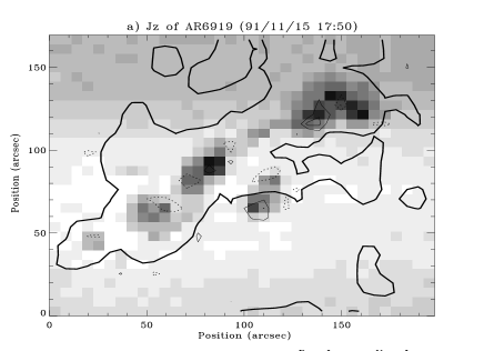
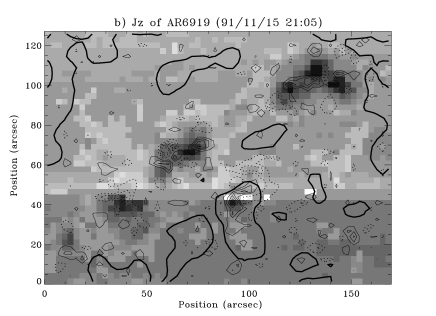
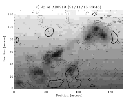
Figure 3: Vertical current densities of AR 6919 superposed on white light images. The contour levels correspond to 3, 6, 9, 12 and 15 $\rm mA/m^{2}$, respectively. Thick solid lines represent the inversion lines inferred from the longitudinal magnetic field data.

We show the vertical current density and inversion lines inferred from the longitudinal fields in Figure 3. As seen in Figures 3-b) and 3-c), the strongest vertical current density kernel is located near the inversion line of the $\delta$ sunspot. As seen in the figures, the vertical current density much increased just before the onset of the X-class flare.

Figure 4: Contours of angular shear multiplied by horizontal field strength obtained from three vector magnetograms of AR 6919 on Nov. 15, 1991 drawn in thick solid lines are superposed on the vertical magnetograms. (thick solid lines) The contour levels are 30000, 40000, 50000 and 60000 G deg, respectively. In all the figures, the thin solid lines stand for positive polarities and the thin dotted lines for negative polarities. The contour levels in the magnetograms correspond to 100, 200, 400, 800 and 1600 G, respectively.

Figure 5: Contours of shear angle multiplied by field strength drawn in thick solid lines are superposed on the vertical magnetograms. The contour levels are 30000, 40000, 50000 and 60000 G deg, respectively. The magnetograms are the same as in Figure 4.

Figure 6: Time variation of weighted shear angle and angular shear before and after an X-class flare in AR 6919. In the figure Local $\theta_{a}$ and Local $\theta_{s}$ are weighted shear angles for the $\delta$ sunspot region.

Table II: Weighted mean magnetic shear angle, angular shear and sum of magnetic free energy density for AR 6919 for three different times. All parameters are calculated for pixels with $B_{z}>100G$. The asterisked data are obtained adopting the potential field method for $180^{\circ}$ ambiguity resolution.

Data	$\overline{\theta}_{s}$	local $\overline{\theta}_{s}$	$\overline{\theta}_{a}$	local $\overline{\theta}_{a}$	$\overline{\rho}_{f}[{\rm erg/cm^{3}}]$	local $\overline{\rho}_{f}$	$\sum\rho_{f}[{\rm erg/cm}]$	local $\sum\rho_{f}$
a)	26.6	43.1	42.4	78.8	5.0E3	1.6E4	1.6E23	3.7E22
b)	22.3	55.9	33.5	92.6	3.6E3	1.6E4	1.1E23	2.6E22
c)	23.0	50.5	35.6	83.4	3.0E3	7.9E3	1.3E23	1.3E22
a)*	23.3	30.1	32.4	48.1	4.1E3	9.3E3	1.3E23	2.2E22
b)*	20.2	36.3	28.3	51.2	2.9E3	8.0E3	9.2E22	1.3E22
c)*	21.3	36.8	30.8	56.2	2.6E3	4.7E3	1.1E23	7.8E21

Figure 7: Contours of free energy density obtained from three vector magnetograms of AR 6919 drawn in thick solid lines are superposed on the vertical magnetograms. The contour levels are $1\times 10^{4}$, $2\times 10^{4}$, $3\times 10^{4}$ and $4\times 10^{4}\,\rm erg/cm^{3}$, respectively. The magnetograms are the same as in Figure 4.

Figure 8: Time variation of the planar sum of free energy density before and after an X-class flare of AR 6919. In the figure Local corresponds to a $\delta$ sunspot region.

Figures 4 and 5 show angular shear weighted with transverse field strength and shear angle weighted with total field strength derived from vector magnetograms and computed potential fields (Sakurai, 1992). As seen in the figures, high values of shear angles are located near the $\delta$ spot region. The changes of two mean shear angles with time are given in Figure 6, which shows that shear angles for the $\delta$ spot area (denoted by Local in the figure) increased before the X-class flare and then decreased after it, but those for the whole active region decreased before the flare. It is to be noted that a similar pattern is also found in the evolution of a measure of magnetic field discontinuity, MAD (see Figure 7 in Moon et el. 1999a). The derived mean shear angles are listed in Table II, in which for comparison we also tabulate the corresponding values obtained with the potential field method for $180^{\circ}$ ambiguity resolution. It is interesting that the mean shear angles for the $\delta$ spot area (denoted by local in Table II) obtained with the potential method continuously increased during the flaring activity unlike those obtained with our method. This eloquently demonstrates that totally different conclusions can be drawn on the shear angle evolution throughout a flare, critically depending on the $180^{\circ}$ ambiguity resolution method employed in data reduction.

The magnetic free energy densities are shown in Figure 7. The free energy density near the $\delta$ spot region largely decreased before the flare. We also list mean energy densities and total energy densities in Table II and plot their variations with time in Figure 8. These data indicate that magnetic free energy, at least in the neighborhood of the $\delta$ spot, was indeed released during the flaring process.

It is notably interesting and not easy to understand that in Figures 6 and 8, the curvatures of curves for the whole active region are of opposite sign to those for the local $\delta$ spot region. This may create some skepticism about the conventional picture of the flare mechanism. In Figure 6, where shear angle variations are displayed, the curves (Local $\theta_{a}$ and Local $\theta_{s}$) for the $\delta$ spot region seem to be consistent with the conventional flare picture, according to which the magnetic shear increases to build up free energy until the flare onset and then decreases as free energy being released. The free energy curve for the same $\delta$ spot region in Figure 8, however, shows that the energy decrease started even before the flare onset although a more drastic energy release followed the onset. This indicates that relaxation of the twisted magnetic field mildly starts even hours before the visible flare onset. The decrease of mean shear angle for the whole active region before the flare supports this argument. Why, then, does the local shear increase before the flare? This may be interpreted as development of a current sheet of a macroscopic size in the possible reconnection region near the $\delta$ spot. Magnetic fields tend to take a lowest possible energy state under given constraints. The lowest energy state is expected to have a smooth spatial variation of magnetic field. However, a smooth state may not exist if the field has undergone too much twist. Then, a current sheet must develop in some regions while the field takes a smooth configuration in other regions. The process of current sheet development may be either a pure ideal MHD process as described above or a process involving a lot of small scale magnetic reconnections. The latter process can be analogized with an avalanche of a sand pile initiated by a slide of a few sand grains. This scenario was proposed and investigated by Lu et al. (1991, 1993). The increase of the planar sum of free energy density over the whole active region shown in Figure 8 still requires more investigation. However, this can be also explained within the conventional picture of solar flares. When a magnetic field is twisted, the whole field tends to expand to occupy more volume per flux. The magnetic energy is thus more concentrated near the surface in a potential field than in a twisted field. The increase of the free energy after the flare onset might imply that the coronal field shrinks down while only part of the total free energy is released by the flaring process. However, our speculations based on only one flare case study definitely need to be examined by investigation of more cases.

Section 5 Summary and Conclusion

In this study, we have studied the magnetic nonpotentiality of AR 6919 associated with an X-class flare which occurred on November 15, 1991, using MSO magnetograms. The magnetogram data were obtained before and after the X-class flare using the Haleakala Stokes Polarimeter. A nonlinear least square method was adopted to derive the magnetic field components from the observed Stokes profiles and a multi-step ambiguity solution method was employed to resolve the $180^{\circ}$ ambiguity. From the $180^{\circ}$ ambiguity-resolved vector magnetograms, we have derived a set of physical quantities characterizing the field configuration. The results emerging from this study can be summarized as follows:

1) There was flux decreases for both polarities in a $\delta$ sunspot pair as well as flux increases outside it, which implies that the energy release of the X-class flare should be associated with flux cancellation and emergence.

2) It was found that the vertical current near the $\delta$ sunspot much increased before the flare.

3) We also found that magnetic shear near the $\delta$ sunspot increased before the flare and then decreased after it, while magnetic shear in the whole active region decreased before the flare.

4) The sum of magnetic energy density decreased before the flare, indicating that magnetic free energy was released by the flaring event.

However, we also found different evolutionary tendencies of nonpotentiality parameters for the whole active region and for the local $\delta$ spot region. These differences must be examined through further studies of many other flare-bearing active regions. If some of them could be confirmed, these would serve as important clues to understand flaring mechanisms.

References

- Ambastha et al. 1993 Ambastha, A., Hagyard, M. J., and West, E. A.: 1993, Solar Phys. 148, 277.
- Canfield et al. 1992 Canfield, R. C., Hudson, H. S., Leka, K. D., Mickey, D. L., Metcalf, T. R., Wülser, J-P., Acton, L. W., Strong, K. T., Kosugi, T., Sakao, T., Tsuneta, S., Culhane, J. L., Phillips, A., and Fludra, A.: 1992, Pub. Astron. Soc. Japan 44, L111.
- Canfield et al. 1993 Canfield, R. C., La Beaujardiere, J.-F., Han, Y., Leka, K. D., McClymont, A. N., Metcalf, T. R., Mickey, D. L., Wülser, J.-P., and Lites, B. W.: 1993, Astrophys. J. 411, 362.
- Canfield and Reardon 1998 Canfield, R. C. and Reardon, K. P.: 1998, Solar Phys. 182, 145.
- Chen et al. 1994 Chen, J., Wang, H., Zirin, H, and Ai, G.: 1994, Solar Phys. 154, 261.
- Gary et al. 1987 Gary, G. A., Moore, R. L., Hagyard, M. J., and Haisch, B. M.: 1987, Astrophys. J. 314, 782.
- Gary et al. 1991 Gary, G. A., Hagyard, M. J., and West, E. A.: 1991, in L. November (ed.), Solar Polarimetry, Proceeding of the Workshop of Solar Polarimetry, p. 65.
- Hagyard et al. 1981 Hagyard, M. J., Low, B. C., and Tandberg-Hanssen, E.: 1981, Solar Phys. 73, 257.
- Hagyard et al. 1982 Hagyard, M. J., Cummings, N. P., West E. A., and Smith, Jr., J. B.: 1982, Solar Phys. 80, 33.
- Hagyard et al. 1984 Hagyard, M. J., Smith, Jr., J. B., Teuber, D., and West, E. A.: 1984, Solar Phys. 91, 115.
- Hagyard et al. 1988 Hagyard, M. J., Gary, G. A., and West, E. A.: 1988, The SAMEX Vector Magnetograph, NASA Technical Memorandum 4048
- Hagyard et al. 1990 Hagyard, M. J., Ventkatarishnan, P., and Smith, Jr., J. B.: 1990, Astrophys. J. Suppl. 73, 159.
- Hagyard et al. 1993 Hagyard, M. J., West, E. A., and Smith, J. E.: 1993, Solar Phys. 144,141.
- Hagyard and Kineke 1995 Hagyard, M. J. and Kineke, J. I.: 1995, Solar Phys. 158, 11.
- Hudson et al. 1992 Hudson, H. S., Acton, L. W., Hirayama, T., and Uchida, Y.: 1992, Pub. Astron. Soc. Japan 44, 77.
- Jefferies and Mickey 1991 Jefferies, J. T. and Mickey, D. L.: 1991, Astrophys. J. 372, 694.
- Kim 1997 Kim, K. S.: 1997, Pub. Korean Astron. Soc. 12, 1.
- Lu et al. 1991 Lu, E. T. and Hamilton, R. J.: 1991, Astrophys. J. 380, L89.
- Lu et al. 1993 Lu, E. T., Hamilton, R. J., McTiernan, J. M., and Bromund, K. R.: 1993, Astrophys. J. 412, 841.
- Lü et al. 1993 Lü, Y., Wang, J., and Wang, H.: 1993, Solar Phys. 148, 119.
- McClymont, Jiao, and Mickić 1997 McClymont, A. N. Jiao, L., and Mickić, Z.: 1997, Solar Phys. 174, 191.
- Metcalf et al. 1995 Metcalf, T. R., Jiao, L., McClymont, A. N., Canfield, R. C., and Uitenbroek, H.: 1995, Astrophys. J. 439, 474.
- Mickey 1985 Mickey, D. L.: 1985, Solar Phys. 97, 223.
- Moon et al. 1999a Moon, Y.-J., Yun, H. S., Lee, S. W., Kim, J.-H. Choe, G. S., Park, Y .D., Ai, G., Zhang, H., and Fang, C.: 1999a, Solar Phys. 184, 323.
- Moon et al. 1999b Moon, Y.-J., Park, Y. D., and Yun, H. S.: 1999b, J. Korean Astron. Soc. 32, 63.
- Moon et al. 1999c Moon, Y.-J., Yun, H. S., Choe, G. S., Park, Y .D., Mickey, D. L.: 1999c, submitted to Solar Physics.
- Ronan et al. 1987 Ronan, R. S., Mickey, D. L., and Orral, F. Q.: 1987, Solar Phys. 113, 353.
- Sakao 1992 Sakao, T., Kosugi, T., Masuda, S., Inda, M, Makishima, K., Canfield, R. C., Hudson, H. S., Metcalf, T. R., Wülser, J.-P., Acton, L. W., Ogawara, Y.: 1992, Pub. Astron. Soc. Japan 44, L83.
- Sakurai 1992 Sakurai, T.: 1992, in his numerical routines
- Sakurai et al. 1995 Sakurai, T., Ichimoto, K,. Nishino, Y., Shinoda, K., Noguchi, M., Hiei, E., Li, T., He, F., Mao, W., Lu, H., Ai, G., Zhao, Z., Kawakami, S., and Chae, J.: 1995, Pub. Astron. Soc. Japan 47, 81.
- Skumanich and Lites 1987 Skumanich, A. and Lites, B. W.: 1987, Astrophys. J. 322, 473.
- Wang 1992 Wang, H.: 1992, Solar Phys. 140, 85.
- Wang and Tang 1993 Wang, H. and Tang, F.: 1993, Astrophys. J. 407, L89.
- Wang et al. 1994 Wang, H., Ewell, W., Zirin, H., and Ai, G.: 1994, Astrophys. J. 424, 436.
- Wang 1997 Wang, H.: 1997, Solar Phys. 174, 163.
- Wang et al. 1996 Wang, J., Shi, Z., Wang, H., and Lu, Y.: 1996, Astrophys. J. 456, 861.
- Wülser et al. 1994 Wülser, J.-P., Canfield, R. C., Actor, L. W., Culhane, J. L., Philips, A., Fludra, A., Sakao, T., Masuda, S., Kosugi, T., and Tsuneta, S.: 1994, Astrophys. J. 424, 459.
- Zirin 1995 Zirin, H.: 1995, Solar Phys. 159, 203.